Exact solution of Markovian master equations for quadratic fermi systems: thermal baths, open XY spin chains, and non-equilibrium phase transition

Tomaž Prosen and Bojan Žunkovič Department of physics, FMF, University of Ljubljana, Jadranska 19, SI-1000 Ljubljana, Slovenia
Abstract

We generalize the method of third quantization to a unified exact treatment of Redfield and Lindblad master equations for open quadratic systems of n𝑛n fermions in terms of diagonalization of 4n×4n4𝑛4𝑛4n\times 4n matrix. Non-equilibrium thermal driving in terms of the Redfield equation is analyzed in detail. We explain how to compute all physically relevant quantities, such as non-equilibrium expectation values of local observables, various entropies or information measures, or time evolution and properties of relaxation. We also discuss how to exactly treat explicitly time dependent problems. The general formalism is then applied to study a thermally driven open XY spin 1/2 chain. We find that recently proposed non-equilibrium quantum phase transition in the open XY chain survives the thermal driving within the Redfield model. In particular, the phase of long-range magnetic correlations can be characterized by hypersensitivity of the non-equilibrium-steady state to external (bath or bulk) parameters. Studying the heat transport we find negative thermal conductance for sufficiently strong thermal driving, as well as non-monotonic dependence of the heat current on the strength of the bath coupling.

pacs:
02.30.Ik, 03.65.Yz, 05.30.Fk, 75.10.Pq

1 Introduction

One of the main challenges of the many-body theory and non-equilibrium statistical mechanics is to understand the properties of relaxation of large interacting quantum systems. There are two common approaches to this type of problems. One important direction is to try to define dynamics in the thermodynamic limit and to investigate its properties with rigorous mathematical methods of operator algebras [1, 2, 3]. However, in this context explicit results which go beyond existence proofs are quite limited. A second approach is to split a large system into a tensor product of a smaller system of interest, and the rest (environment), and trying to eliminate all the degrees of freedom of the large, macroscopic environment (see e.g. [4, 5]). This approach, although involving a series of approximations, is usually more fruitful for explicit calculations and quantitative analyses. We may be interested either in relaxation to equilibrium or non-equilibrium steady states, depending on the equal or non-equal values of thermodynamic potentials assigned to possibly several pieces of environment - which we shall call the baths. Such calculations of the quantitative properties of steady states may be very useful, for example in the realm of transport theory [6] as may complement the linear response calculations and suggest non-linear response or far-from-equilibrium effects.

However, to date we have had a very few explicit calculations of non-equilibrium properties of open many body quantum systems, and mainly they had to focus on small systems with a single or a pair of degrees of freedoms (such as spins, or bosons), see for example [7, 8]. The reason is that there has been no theoretical techniques to deal with open many-body problems except for the Keldysh formalism of non-equilibrium Green’s functions, which however can easily get too involved for explicit calculations. Recently, two new directions have been proposed, both in the direction of numerical simulation and theoretical analysis. Namely, in the context of numerical simulations of open many-body systems, time-dependent density matrix renormalization group techniques [9] have been demonstrated to efficiently simulate relaxation to steady states with the Lindblad master equation [10]. On the other hand, it has been shown [11] that the Lindblad equation for general quadratic fermionic systems, for example for XY-like quantum spin chains which are mappable to quadratic fermionic systems, can be solved explicitly with the technique of canonical quantization in the Fock space of operators - third quantization for short.

In this paper we shall show how the third quantization can be generalized to treat quadratic systems with arbitrary Markovian master equations , which is not necessarily of the Lindblad form. In particular, we shall focus on the Redfield dissipator in terms of which we can simulate simple thermal reservoirs, and thermal driving of the system under non-equilibrium conditions. After giving a short account on mathematical formulation of Markovian master equations and the basic physical assumptions and approximations involved in the derivation - in section 2, we shall in section 3 present a short but self-contained generalization of the theory [11]. In addition, we shall outline the calculation of dynamical correlation functions in Liouvillean dynamics, and formulate an exact treatment of explicitly time-dependent quantum Liouville problems. In section 4 we shall apply our technique to treat an open XY spin chain in the non-equilibrium Redfield model. We shall outline several intriguing exact numerical results on large spin chains. In particular, we show that recently announced quantum phase transition in the open XY chain in the local Lindblad bath model, generalizes also to non-equilibrium thermal Redfield model with qualitatively identical characteristics. The transition is characterized by spontaneous emergence of long range magnetic correlations, and hypersensitivity of the steady state to external system’s parameters, when the transverse magnetic field drops bellow the critical value |h|<hc=|1γ2|subscriptc1superscript𝛾2|h|<h_{\rm c}=|1-\gamma^{2}| where γ𝛾\gamma is the anisotropy parameter. Furthermore, we analyze in some detail the heat transport in XY chain, and find regions of negative differential heat conductance for strong thermal driving, namely non-monotonic dependence of the heat current on the temperature difference between the baths.

2 Markovian master equations in non-equilibrium quantum physics

Decomposing the Hilbert space of the universe into a tensor product =sbtensor-productsubscriptssubscriptb{\cal H}={\cal H}_{\rm s}\otimes{\cal H}_{\rm b} of the central system ssubscripts{\cal H}_{\rm s} and the bath (or a set of baths) bsubscriptb{\cal H}_{\rm b} (environment), one writes the total Hamiltonian as

H=Hs𝟙b+𝟙sHb+λμXμYμ,𝐻tensor-productsubscript𝐻ssubscript1btensor-productsubscript1ssubscript𝐻b𝜆subscript𝜇tensor-productsubscript𝑋𝜇subscript𝑌𝜇H=H_{\rm s}\otimes\mathbbm{1}_{\rm b}+\mathbbm{1}_{\rm s}\otimes H_{\rm b}+\lambda\sum_{\mu}X_{\mu}\otimes Y_{\mu}, (1)

where Xμsubscript𝑋𝜇X_{\mu}, are linear operators over ssubscripts{\cal H}_{\rm s}, and Yμsubscript𝑌𝜇Y_{\mu} linear operators over bsubscriptb{\cal H}_{\rm b}. Note that Xμ,Yμsubscript𝑋𝜇subscript𝑌𝜇X_{\mu},Y_{\mu} can always be chosen to be Hermitian, so this shall be assumed throughout this paper. The Markovian quantum master equation for the time evolution of the central systems’s density matrix ρ(t)𝜌𝑡\rho(t) is derived [4] using three main assumptions: (i) weak coupling (assuming λ𝜆\lambda to be small), (ii) factorizability of the initial density matrix ρs(0)ρb(0)tensor-productsubscript𝜌s0subscript𝜌b0\rho_{\rm s}(0)\otimes\rho_{\rm b}(0), and (iii) Born-Markov approximation which rests upon the assumption that the bath-correlation functions

Γμ,νβ(t):=λ2tr(Y~μ(t)YνeβHb)/treβHb,Y~μ(t):=eitHbYμeitHbformulae-sequenceassignsubscriptsuperscriptΓ𝛽𝜇𝜈𝑡superscript𝜆2trsubscript~𝑌𝜇𝑡subscript𝑌𝜈superscript𝑒𝛽subscript𝐻btrsuperscript𝑒𝛽subscript𝐻bassignsubscript~𝑌𝜇𝑡superscript𝑒i𝑡subscript𝐻bsubscript𝑌𝜇superscript𝑒i𝑡subscript𝐻b\Gamma^{\beta}_{\mu,\nu}(t):=\lambda^{2}{\,{\rm tr}\,}(\tilde{Y}_{\mu}(t)Y_{\nu}e^{-\beta H_{\rm b}})/{\,{\rm tr}\,}e^{-\beta H_{\rm b}},\quad\tilde{Y}_{\mu}(t):=e^{{\rm i}tH_{\rm b}}Y_{\mu}e^{-{\rm i}tH_{\rm b}} (2)

decay on much shorter time scale than the central systems dynamics X~μ(t):=eitHsXμeitHsassignsubscript~𝑋𝜇𝑡superscript𝑒i𝑡subscript𝐻ssubscript𝑋𝜇superscript𝑒i𝑡subscript𝐻s\tilde{X}_{\mu}(t):=e^{{\rm i}tH_{\rm s}}X_{\mu}e^{-{\rm i}tH_{\rm s}}. We use units in which Planck’s constant =1Planck-constant-over-2-pi1\hbar=1, and may use different inverse temperatures β𝛽\beta for different pieces of the environment (for different baths). The resulting master equation is referred to as the Redfield equation

ddtρ(t)=i[Hs,ρ(t)]+𝒟^ρ(t),dd𝑡𝜌𝑡isubscript𝐻s𝜌𝑡^𝒟𝜌𝑡\frac{{\rm d}}{{\rm d}t}\rho(t)=-{\rm i}[H_{\rm s},\rho(t)]+\hat{\cal D}\rho(t), (3)

where the dissipator-map has a memoryless kernel with the following general form

𝒟^ρ=μ,ν0dτΓν,μβ(τ)[X~μ(τ)ρ,Xν]+h.c.formulae-sequence^𝒟𝜌subscript𝜇𝜈superscriptsubscript0differential-d𝜏superscriptsubscriptΓ𝜈𝜇𝛽𝜏subscript~𝑋𝜇𝜏𝜌subscript𝑋𝜈𝑐\hat{\cal D}\rho=\sum_{\mu,\nu}\int_{0}^{\infty}{\rm d}\tau\Gamma_{\nu,\mu}^{\beta}(\tau)[\tilde{X}_{\mu}(-\tau)\rho,X_{\nu}]+h.c. (4)

If one additionally assumes the so-called rotating wave-approximation, one arrives at the dynamical semi-group which manifestly preserves the positivity of density matrix at all times111This is not the case for equation (3,4) which allows for possible breaking of positivity at initial short time interval, the so called sleapage time. and can be generally described by the dissipator in the Lindblad form

𝒟^ρ=μ,νγν,μ[Xμρ,Xν]+h.c.,formulae-sequencesuperscript^𝒟𝜌subscript𝜇𝜈subscript𝛾𝜈𝜇subscript𝑋𝜇𝜌subscript𝑋𝜈𝑐\hat{\cal D}^{\prime}\rho=\sum_{\mu,\nu}\gamma_{\nu,\mu}[X_{\mu}\rho,X_{\nu}]+h.c., (5)

where the only condition is that γ𝛾{\mathbf{\gamma}} is a Hermitian γμ,ν=γν,μsubscript𝛾𝜇𝜈subscriptsuperscript𝛾𝜈𝜇\gamma_{\mu,\nu}=\gamma^{*}_{\nu,\mu} and positive definite matrix. The standard Lindblad form is obtained by diagonalizing the matrix γ𝛾{\mathbf{\gamma}} whose eigenvectors yield the usual Lindblad operators. The important property of the bath-correlation functions (2) (which constitute all that we need to know about the baths) is the Kubo-Martin-Schwinger(KMS) condition

Γμ,νβ(tiβ)=Γν,μβ(t),subscriptsuperscriptΓ𝛽𝜇𝜈𝑡i𝛽subscriptsuperscriptΓ𝛽𝜈𝜇𝑡\Gamma^{\beta}_{\mu,\nu}(-t-{\rm i}\beta)=\Gamma^{\beta}_{\nu,\mu}(t), (6)

which is needed to prove that the thermal state ρgibbs=eβHs/treβHssubscript𝜌gibbssuperscript𝑒𝛽subscript𝐻strsuperscript𝑒𝛽subscript𝐻s\rho_{\rm gibbs}=e^{-\beta H_{\rm s}}/{\,{\rm tr}\,}e^{-\beta H_{\rm s}} is a steady state of the master equation (3), provided that all baths are thermalized to the same inverse temperature222With an additional technical condition of neglecting the Cauchy principal value contribution to the time integral 4, see the discussion at the end of subsection 3.2. However, in case of several thermal baths with possibly different temperatures we may expect that ρ(t)𝜌𝑡\rho(t) relaxes to a physically very interesting non-equilibrium-steady-state (NESS).

3 Diagonalization of quantum Liouvilleans for quadratic fermi systems

In this section we give a short account on the general technique of canonical quantization in the Liouvile space (‘third quantization’) and complete diagonalization of Markovian master equations (3), with (4) or (5), for quadratic fermionic problems. We treat a finite problem with n𝑛n fermionic degrees of freedom, described by 2n2𝑛2n anti-comuting Hermitian operators wjsubscript𝑤𝑗w_{j}, j=1,2,,2n𝑗122𝑛j=1,2,\ldots,2n, {wj,wk}=2δj,ksubscript𝑤𝑗subscript𝑤𝑘2subscript𝛿𝑗𝑘\{w_{j},w_{k}\}=2\delta_{j,k}, in which the Hamiltonian H𝐻H may take a general quadratic form and the coupling operators may be general linear forms:

Hssubscript𝐻s\displaystyle H_{\rm s} =\displaystyle= j,k=12nwjHj,kwk=w¯𝐇w¯,superscriptsubscript𝑗𝑘12𝑛subscript𝑤𝑗subscript𝐻𝑗𝑘subscript𝑤𝑘¯𝑤𝐇¯𝑤\displaystyle\sum_{j,k=1}^{2n}w_{j}H_{j,k}w_{k}={\underline{w}}\cdot{\mathbf{H}}\,{\underline{w}}, (7)
Xμsubscript𝑋𝜇\displaystyle X_{\mu} =\displaystyle= j=12nxμ,jwj=x¯μw¯.superscriptsubscript𝑗12𝑛subscript𝑥𝜇𝑗subscript𝑤𝑗subscript¯𝑥𝜇¯𝑤\displaystyle\sum_{j=1}^{2n}x_{\mu,j}w_{j}={\underline{x}}_{\mu}\cdot{\underline{w}}\ . (8)

Thus, 2n×2n2𝑛2𝑛2n\times 2n matrix 𝐇𝐇{\mathbf{H}} can be chosen to be antisymmetric 𝐇T=𝐇superscript𝐇𝑇𝐇{\mathbf{H}}^{T}=-{\mathbf{H}}. Throughout this paper x¯=(x1,x2,)T¯𝑥superscriptsubscript𝑥1subscript𝑥2𝑇{\underline{x}}=(x_{1},x_{2},\ldots)^{T} will designate a vector (column) of appropriate scalar valued or operator valued symbols xksubscript𝑥𝑘x_{k}. This formalism is immedately applicable either for describing, (i) physical fermions cmsubscript𝑐𝑚c_{m}, m=1,2,,n𝑚12𝑛m=1,2,\ldots,n, where w2m1=cm+cmsubscript𝑤2𝑚1subscript𝑐𝑚superscriptsubscript𝑐𝑚w_{2m-1}=c_{m}+c_{m}^{\dagger}, w2m=i(cmcm)subscript𝑤2𝑚isubscript𝑐𝑚subscriptsuperscript𝑐𝑚w_{2m}={\rm i}(c_{m}-c^{\dagger}_{m}), or (ii) XY-like systems of spins 1/2121/2 with canonical Pauli operators σmsubscript𝜎𝑚\vec{\sigma}_{m}, m=1,2,,n𝑚12𝑛m=1,2,\ldots,n, where the fermionic operators are represented by the famous Jordan-Wigner transformation

w2m1=σmxm<mσmz,w2m=σmym<mσmz.formulae-sequencesubscript𝑤2𝑚1subscriptsuperscript𝜎x𝑚subscriptproductsuperscript𝑚𝑚subscriptsuperscript𝜎zsuperscript𝑚subscript𝑤2𝑚subscriptsuperscript𝜎y𝑚subscriptproductsuperscript𝑚𝑚subscriptsuperscript𝜎zsuperscript𝑚w_{2m-1}=\sigma^{\rm x}_{m}\prod_{m^{\prime}<m}\sigma^{\rm z}_{m^{\prime}}\,,\qquad w_{2m}=\sigma^{\rm y}_{m}\prod_{m^{\prime}<m}\sigma^{\rm z}_{m^{\prime}}\,. (9)

3.1 Fock space of operators

The fundamental concept for our analysis is a Fock space structure over the 4nsuperscript4𝑛4^{n} dimensional Liouville space of operators 𝒦𝒦{\cal K}, which density matrix ρ(t)𝜌𝑡\rho(t) is also a member of. From here on, we shall adopt Dirac bra-ket notation for the operator space 𝒦𝒦{\cal K} which is fixed by the following definition of the inner product

x|y=trxy,x,y𝒦.formulae-sequenceinner-product𝑥𝑦trsuperscript𝑥𝑦𝑥𝑦𝒦\langle x|y\rangle={\,{\rm tr}\,}x^{\dagger}y,\qquad x,y\in{\cal K}. (10)

We note that 22nsuperscript22𝑛2^{2n} operator-products |Pα¯ketsubscript𝑃¯𝛼{|P_{{\underline{\alpha}}}\rangle}, labelled with a binary multi-index α¯¯𝛼{\underline{\alpha}}

Pα1,α2,,α2n:=2n/2w1α1w2α2w2nα2n,αj{0,1}formulae-sequenceassignsubscript𝑃subscript𝛼1subscript𝛼2subscript𝛼2𝑛superscript2𝑛2superscriptsubscript𝑤1subscript𝛼1superscriptsubscript𝑤2subscript𝛼2superscriptsubscript𝑤2𝑛subscript𝛼2𝑛subscript𝛼𝑗01P_{\alpha_{1},\alpha_{2},\ldots,\alpha_{2n}}:=2^{-n/2}w_{1}^{\alpha_{1}}w_{2}^{\alpha_{2}}\cdots w_{2n}^{\alpha_{2n}},\qquad\alpha_{j}\in\{0,1\} (11)

constitute a complete orthonormal basis of 𝒦𝒦{\cal K} with respect to an inner product.

In fact it is easy to show that |Pα¯ketsubscript𝑃¯𝛼{|P_{{\underline{\alpha}}}\rangle} is a fermionic Fock basis, and powers 111 in the product (11) can be considered like a sort of Fermionic excitations, if we define the following set of linear annihilation maps c^jsubscript^𝑐𝑗\hat{c}_{j} over333We shall use notation where linear maps over the operator space (in physics literature sometimes referred to as “super-operators”) are designated by ^^absent\hat{}. 𝒦𝒦{\cal K}

c^j|Pα¯=αj|wjPα¯,subscript^𝑐𝑗ketsubscript𝑃¯𝛼subscript𝛼𝑗ketsubscript𝑤𝑗subscript𝑃¯𝛼{\hat{c}}_{j}{|P_{{\underline{\alpha}}}\rangle}=\alpha_{j}{|w_{j}P_{{\underline{\alpha}}}\rangle}, (12)

and derive the actions of their Hermitian adjoints - the creation linear maps c^superscript^𝑐\hat{c}^{\dagger},

c^j|Pα¯=(1αj)|wjPα¯,subscriptsuperscript^𝑐𝑗ketsubscript𝑃¯𝛼1subscript𝛼𝑗ketsubscript𝑤𝑗subscript𝑃¯𝛼{\hat{c}}^{\dagger}_{j}{|P_{{\underline{\alpha}}}\rangle}=(1-\alpha_{j}){|w_{j}P_{{\underline{\alpha}}}\rangle}, (13)

which satisfy canonical anticommutation relations

{c^j,c^k}=0,{c^j,c^k}=δj,k,j,k=1,2,,2n.formulae-sequencesubscript^𝑐𝑗subscript^𝑐𝑘0formulae-sequencesubscript^𝑐𝑗superscriptsubscript^𝑐𝑘subscript𝛿𝑗𝑘𝑗𝑘122𝑛\{{\hat{c}}_{j},{\hat{c}}_{k}\}=0,\qquad\{{\hat{c}}_{j},{\hat{c}}_{k}^{\dagger}\}=\delta_{j,k},\qquad j,k=1,2,\ldots,2n. (14)

3.2 Bilinear form of the Liouvillean

The aim is now to show that the generator of the master equation (3)

^:=iadH+𝒟^assign^iad𝐻^𝒟{\hat{\cal L}}:=-{\rm i}{\,{\rm ad}\,}H+{\hat{\cal D}} (15)

is in general a quadratic form in these adjoint fermionic maps c^j,c^jsubscript^𝑐𝑗subscriptsuperscript^𝑐𝑗\hat{c}_{j},\hat{c}^{\dagger}_{j}. In order to see that clearly, let us define the left and right multiplication maps over 𝒦𝒦{\cal K}

w^jL|x:=|wjx,w^jR|x:=|xwj.formulae-sequenceassignsubscriptsuperscript^𝑤L𝑗ket𝑥ketsubscript𝑤𝑗𝑥assignsubscriptsuperscript^𝑤R𝑗ket𝑥ket𝑥subscript𝑤𝑗\hat{w}^{\rm L}_{j}{|x\rangle}:={|w_{j}x\rangle},\qquad\hat{w}^{\rm R}_{j}{|x\rangle}:={|xw_{j}\rangle}. (16)

Inspecting the actions of w^jL,w^jRsubscriptsuperscript^𝑤L𝑗subscriptsuperscript^𝑤R𝑗\hat{w}^{\rm L}_{j},\hat{w}^{\rm R}_{j} on the Fock basis |Pα¯ketsubscript𝑃¯𝛼{|P_{{\underline{\alpha}}}\rangle} one arrives at the following useful identities

w^jLsubscriptsuperscript^𝑤L𝑗\displaystyle\hat{w}^{\rm L}_{j} =\displaystyle= c^j+c^j,subscript^𝑐𝑗superscriptsubscript^𝑐𝑗\displaystyle\hat{c}_{j}+\hat{c}_{j}^{\dagger}, (17)
w^jRsubscriptsuperscript^𝑤R𝑗\displaystyle\hat{w}^{\rm R}_{j} =\displaystyle= 𝒫^(c^jc^j)=(c^jc^j)𝒫^,^𝒫subscript^𝑐𝑗superscriptsubscript^𝑐𝑗subscript^𝑐𝑗superscriptsubscript^𝑐𝑗^𝒫\displaystyle{\hat{\cal P}}(\hat{c}_{j}-\hat{c}_{j}^{\dagger})=-(\hat{c}_{j}-\hat{c}_{j}^{\dagger}){\hat{\cal P}}, (18)

where

𝒫^:=exp(iπ𝒩^),and𝒩^:=j=12nc^jc^jformulae-sequenceassign^𝒫i𝜋^𝒩andassign^𝒩superscriptsubscript𝑗12𝑛subscriptsuperscript^𝑐𝑗subscript^𝑐𝑗{\hat{\cal P}}:=\exp({\rm i}\pi{\hat{\cal N}}),{\quad\rm and\quad}{\hat{\cal N}}:=\sum_{j=1}^{2n}\hat{c}^{\dagger}_{j}\hat{c}_{j} (19)

are a parity map, and a number map, respectively, which count the parity and number of the adjoint fermionic excitations (number of factors in (11)). Note that 𝒫^^𝒫{\hat{\cal P}}, anticommutes with all c^j,c^jsubscript^𝑐𝑗subscriptsuperscript^𝑐𝑗\hat{c}_{j},\hat{c}^{\dagger}_{j}, hence the second equality of (18), and 𝒫^2=𝟙^superscript^𝒫2^1{\hat{\cal P}}^{2}=\hat{\mathbbm{1}}.

The unitary part of the Liouvillean (15) now trivially reads

iadHs=iw¯^L𝐇w¯^L+i𝐇w¯^Rw¯^R=4ic¯^𝐇c¯^.iadsubscript𝐻sisuperscript¯^𝑤L𝐇superscript¯^𝑤Li𝐇superscript¯^𝑤Rsuperscript¯^𝑤R4isuperscript¯^𝑐𝐇¯^𝑐-{\rm i}{\,{\rm ad}\,}H_{\rm s}=-{\rm i}{\underline{\hat{w}}}^{\rm L}\cdot{\mathbf{H}}{\underline{\hat{w}}}^{\rm L}+{\rm i}{\mathbf{H}}{\underline{\hat{w}}}^{\rm R}\cdot{\underline{\hat{w}}}^{\rm R}=-4{\rm i}{\underline{\hat{c}}}^{\dagger}\cdot{\mathbf{H}}{\underline{\hat{c}}}\,. (20)

The dissipator (4) can be represented as a map over 𝒦𝒦{\cal K} as

𝒟^=μ,νj,k=12nxν,k0dτfμ,j(τ)(Γν,μβ(τ)^j,k+Γν,μβ(τ)^j,k′′),^𝒟subscript𝜇𝜈superscriptsubscript𝑗𝑘12𝑛subscript𝑥𝜈𝑘superscriptsubscript0differential-d𝜏subscript𝑓𝜇𝑗𝜏superscriptsubscriptΓ𝜈𝜇𝛽𝜏subscriptsuperscript^𝑗𝑘superscriptsubscriptΓ𝜈𝜇𝛽𝜏subscriptsuperscript^′′𝑗𝑘\!\!\!\!\!\!\!\!\!\!\!{\hat{\cal D}}=\sum_{\mu,\nu}\sum_{j,k=1}^{2n}x_{\nu,k}\int_{0}^{\infty}\!\!\!{\rm d}\tau f_{\mu,j}(-\tau)\left(\Gamma_{\nu,\mu}^{\beta}(\tau){\hat{\cal L}}^{\prime}_{j,k}+\Gamma_{\nu,\mu}^{\beta*}(\tau){\hat{\cal L}}^{\prime\prime}_{j,k}\right), (21)

where f¯μ(t)subscript¯𝑓𝜇𝑡{\underline{f}}_{\mu}(t) is a (real-valued) propagator of Heisenberg dynamics in the closed system

X~μ(t)=x¯μexp(iadHst)w¯=:f¯μ(t)w¯,\tilde{X}_{\mu}(t)={\underline{x}}_{\mu}\cdot\exp(-{\rm i}{\,{\rm ad}\,}H_{\rm s}t){\underline{w}}=:{\underline{f}}_{\mu}(t)\cdot{\underline{w}}, (22)

which - due to (20) - can be explicitly solved for a quadratic Hamiltonian (7), giving

f¯μ(t)=exp(4i𝐇t)x¯μ,subscript¯𝑓𝜇𝑡4i𝐇𝑡subscript¯𝑥𝜇{\underline{f}}_{\mu}(t)=\exp(4{\rm i}{\mathbf{H}}t){\underline{x}}_{\mu}, (23)

and

^j,k|x:=|[wjx,wk],^j,k′′|x:=|[wk,xwj]formulae-sequenceassignsubscriptsuperscript^𝑗𝑘ket𝑥ketsubscript𝑤𝑗𝑥subscript𝑤𝑘assignsubscriptsuperscript^′′𝑗𝑘ket𝑥ketsubscript𝑤𝑘𝑥subscript𝑤𝑗{\hat{\cal L}}^{\prime}_{j,k}{|x\rangle}:={|[w_{j}x,w_{k}]\rangle},\quad{\hat{\cal L}}^{\prime\prime}_{j,k}{|x\rangle}:={|[w_{k},xw_{j}]\rangle} (24)

are fundamental basis dissipators which using (17,18) evaluate to

^j,ksubscriptsuperscript^𝑗𝑘\displaystyle\!\!\!\!\!\!\!\!\!\!{\hat{\cal L}}^{\prime}_{j,k} =\displaystyle= w^jLw^kRw^kLw^jL=(𝟙^+𝒫^)(c^jc^kc^kc^j)+(𝟙^𝒫^)(c^jc^kc^kc^j),subscriptsuperscript^𝑤L𝑗subscriptsuperscript^𝑤R𝑘subscriptsuperscript^𝑤L𝑘subscriptsuperscript^𝑤L𝑗^1^𝒫subscriptsuperscript^𝑐𝑗subscriptsuperscript^𝑐𝑘subscriptsuperscript^𝑐𝑘subscript^𝑐𝑗^1^𝒫subscript^𝑐𝑗subscript^𝑐𝑘subscript^𝑐𝑘subscriptsuperscript^𝑐𝑗\displaystyle\hat{w}^{\rm L}_{j}\hat{w}^{\rm R}_{k}-\hat{w}^{\rm L}_{k}\hat{w}^{\rm L}_{j}=(\hat{\mathbbm{1}}+{\hat{\cal P}})(\hat{c}^{\dagger}_{j}\hat{c}^{\dagger}_{k}-\hat{c}^{\dagger}_{k}\hat{c}_{j})+(\hat{\mathbbm{1}}-{\hat{\cal P}})(\hat{c}_{j}\hat{c}_{k}-\hat{c}_{k}\hat{c}^{\dagger}_{j}), (25)
^j,k′′subscriptsuperscript^′′𝑗𝑘\displaystyle\!\!\!\!\!\!\!\!\!\!{\hat{\cal L}}^{\prime\prime}_{j,k} =\displaystyle= w^kLw^jRw^kRw^jR=(𝟙^+𝒫^)(c^kc^jc^kc^j)+(𝟙^𝒫^)(c^kc^jc^kc^j).subscriptsuperscript^𝑤L𝑘subscriptsuperscript^𝑤R𝑗subscriptsuperscript^𝑤R𝑘subscriptsuperscript^𝑤R𝑗^1^𝒫subscriptsuperscript^𝑐𝑘subscriptsuperscript^𝑐𝑗subscriptsuperscript^𝑐𝑘subscript^𝑐𝑗^1^𝒫subscript^𝑐𝑘subscript^𝑐𝑗subscript^𝑐𝑘subscriptsuperscript^𝑐𝑗\displaystyle\hat{w}^{\rm L}_{k}\hat{w}^{\rm R}_{j}-\hat{w}^{\rm R}_{k}\hat{w}^{\rm R}_{j}=(\hat{\mathbbm{1}}+{\hat{\cal P}})(\hat{c}^{\dagger}_{k}\hat{c}^{\dagger}_{j}-\hat{c}^{\dagger}_{k}\hat{c}_{j})+(\hat{\mathbbm{1}}-{\hat{\cal P}})(\hat{c}_{k}\hat{c}_{j}-\hat{c}_{k}\hat{c}^{\dagger}_{j}). (26)

It will prove useful if we express the internal dynamics (23) explicitly in terms of eigenvalues and eigenvectors of the Hamiltonian matrix 𝐇𝐇{\mathbf{H}}. Since 2n×2n2𝑛2𝑛2n\times 2n matrix is anti-symmetric and Hermitian, its real eigenvalues come in pairs ϵm,ϵm,j=1,,nformulae-sequencesubscriptitalic-ϵ𝑚subscriptitalic-ϵ𝑚𝑗1𝑛\epsilon_{m},-\epsilon_{m},j=1,\ldots,n, with the corresponding eigenvectors u¯m,u¯msubscript¯𝑢𝑚superscriptsubscript¯𝑢𝑚{\underline{u}}_{m},{\underline{u}}_{m}^{*}, namely 𝐇u¯m=ϵmu¯m𝐇subscript¯𝑢𝑚subscriptitalic-ϵ𝑚subscript¯𝑢𝑚{\mathbf{H}}{\underline{u}}_{m}=\epsilon_{m}{\underline{u}}_{m} and 𝐇u¯m=ϵmu¯m𝐇subscriptsuperscript¯𝑢𝑚subscriptitalic-ϵ𝑚subscriptsuperscript¯𝑢𝑚{\mathbf{H}}{\underline{u}}^{*}_{m}=-\epsilon_{m}{\underline{u}}^{*}_{m} since 𝐇=𝐇superscript𝐇𝐇{\mathbf{H}}^{*}=-{\mathbf{H}}. The eigenvectors may and should always be chosen orthonormal (even in the case of degeneracies), meaning

u¯lu¯m=0,u¯lu¯m=δl,m.formulae-sequencesubscript¯𝑢𝑙subscript¯𝑢𝑚0subscript¯𝑢𝑙subscriptsuperscript¯𝑢𝑚subscript𝛿𝑙𝑚{\underline{u}}_{l}\cdot{\underline{u}}_{m}=0,\qquad{\underline{u}}_{l}\cdot{\underline{u}}^{*}_{m}=\delta_{l,m}. (27)

Then the spectral decomposition of the Heisenberg dynamics reads

f¯μ(t)=m=1n(e4iϵmt(x¯μu¯m)u¯m+e4iϵmt(x¯μu¯m)u¯m).subscript¯𝑓𝜇𝑡superscriptsubscript𝑚1𝑛superscript𝑒4isubscriptitalic-ϵ𝑚𝑡subscript¯𝑥𝜇subscript¯𝑢𝑚subscriptsuperscript¯𝑢𝑚superscript𝑒4isubscriptitalic-ϵ𝑚𝑡subscript¯𝑥𝜇subscriptsuperscript¯𝑢𝑚subscript¯𝑢𝑚{\underline{f}}_{\mu}(t)=\sum_{m=1}^{n}\left(e^{-4{\rm i}\epsilon_{m}t}({\underline{x}}_{\mu}\cdot{\underline{u}}_{m}){\underline{u}}^{*}_{m}+e^{4{\rm i}\epsilon_{m}t}({\underline{x}}_{\mu}\cdot{\underline{u}}^{*}_{m}){\underline{u}}_{m}\right). (28)

Note that 𝒫^±=(𝟙^±𝒫^)/2subscript^𝒫plus-or-minusplus-or-minus^1^𝒫2{\hat{\cal P}}_{\pm}=(\hat{\mathbbm{1}}\pm{\hat{\cal P}})/2 are orthogonal projectors which commute with all the terms (20,25,26) that constitute the Liouvillean (15), [𝒫^±,^]=0subscript^𝒫plus-or-minus^0[{\hat{\cal P}}_{\pm},{\hat{\cal L}}]=0, and hence the dynamics (3) does not mix the operator subspaces 𝒦±=𝒫^±𝒦superscript𝒦plus-or-minussubscript^𝒫plus-or-minus𝒦{\cal K}^{\pm}={\hat{\cal P}}_{\pm}{\cal K} composed of even/odd number of fermionic operators. Since we are mainly interested in expectation values of even observables, such as currents and densities, we shall in the present paper focus on the dynamics in the subspace 𝒦+superscript𝒦{\cal K}^{+} only, and consider the corresponding Lioivillean ^|𝒦+evaluated-at^superscript𝒦{\hat{\cal L}}|_{{\cal K}^{+}}

^+=𝒫^+^𝒫^+.subscript^subscript^𝒫^subscript^𝒫{\hat{\cal L}}_{+}={\hat{\cal P}}_{+}{\hat{\cal L}}{\hat{\cal P}}_{+}. (29)

The extension to the odd parity subspace is straightforward. Collecting the results (20,21,25,26) it is now obvious that ^+subscript^{\hat{\cal L}}_{+} is a bilinear form in c^jsubscriptsuperscript^𝑐𝑗\hat{c}^{\dagger}_{j} and c^jsubscript^𝑐𝑗\hat{c}_{j}. For convenience, we define 4n4𝑛4n Hermitian Majorana maps a^r,r=1,4nformulae-sequencesubscript^𝑎𝑟𝑟14𝑛\hat{a}_{r},r=1,\ldots 4n

a^2j1=12(c^j+c^j),a^2j=i2(c^jc^j),formulae-sequencesubscript^𝑎2𝑗112subscript^𝑐𝑗subscriptsuperscript^𝑐𝑗subscript^𝑎2𝑗i2subscript^𝑐𝑗subscriptsuperscript^𝑐𝑗\hat{a}_{2j-1}=\frac{1}{\sqrt{2}}(\hat{c}_{j}+\hat{c}^{\dagger}_{j}),\quad\hat{a}_{2j}=\frac{{\rm i}}{\sqrt{2}}(\hat{c}_{j}-\hat{c}^{\dagger}_{j}), (30)

and express the Liouvillean as

^+=a¯^𝐀a¯^A0𝟙^,subscript^¯^𝑎𝐀¯^𝑎subscript𝐴0^1{\hat{\cal L}}_{+}={\underline{\hat{a}}}\cdot{\mathbf{A}}{\underline{\hat{a}}}-A_{0}\hat{\mathbbm{1}}, (31)

where the 4n×4n4𝑛4𝑛4n\times 4n complex antisymmetrix matrix 𝐀𝐀{\mathbf{A}}, later referred to as a structure matrix, and a scalar A0subscript𝐴0A_{0}, can be expressed as

A2j1,2k1subscript𝐴2𝑗12𝑘1\displaystyle A_{2j-1,2k-1} =\displaystyle= 2iHj,kMj,k+Mk,j,2isubscript𝐻𝑗𝑘subscript𝑀𝑗𝑘subscript𝑀𝑘𝑗\displaystyle-2{\rm i}H_{j,k}-M_{j,k}+M_{k,j}\small,
A2j1,2ksubscript𝐴2𝑗12𝑘\displaystyle A_{2j-1,2k} =\displaystyle= iMk,j+iMj,k,isubscript𝑀𝑘𝑗isuperscriptsubscript𝑀𝑗𝑘\displaystyle\;\;\;\;{\rm i}M_{k,j}+{\rm i}M_{j,k}^{*}\small,
A2j,2k1subscript𝐴2𝑗2𝑘1\displaystyle A_{2j,2k-1} =\displaystyle= iMj,kiMk,j,isubscript𝑀𝑗𝑘isuperscriptsubscript𝑀𝑘𝑗\displaystyle-{\rm i}M_{j,k}-{\rm i}M_{k,j}^{*}\small,
A2j,2ksubscript𝐴2𝑗2𝑘\displaystyle A_{2j,2k} =\displaystyle= 2iHj,kMj,k+Mk,j,2isubscript𝐻𝑗𝑘subscriptsuperscript𝑀𝑗𝑘subscriptsuperscript𝑀𝑘𝑗\displaystyle-2{\rm i}H_{j,k}-M^{*}_{j,k}+M^{*}_{k,j}\small, (32)
A0subscript𝐴0\displaystyle A_{0} =\displaystyle= tr𝐌+tr𝐌,tr𝐌trsuperscript𝐌\displaystyle{\,{\rm tr}\,}{\mathbf{M}}+{\,{\rm tr}\,}{\mathbf{M}}^{*}\small,

where 𝐌𝐌{\mathbf{M}} is a 2n×2n2𝑛2𝑛2n\times 2n bath-matrix which can be compactly written as

𝐌𝐌\displaystyle{\mathbf{M}} :=assign\displaystyle:= νx¯νz¯ν,subscript𝜈tensor-productsubscript¯𝑥𝜈subscript¯𝑧𝜈\displaystyle\sum_{\nu}{\underline{x}}_{\nu}\otimes{\underline{z}}_{\nu}, (33)
z¯νsubscript¯𝑧𝜈\displaystyle{\underline{z}}_{\nu} :=assign\displaystyle:= μ0dτΓν,μβ(τ)f¯μ(τ).subscript𝜇superscriptsubscript0differential-d𝜏subscriptsuperscriptΓ𝛽𝜈𝜇𝜏subscript¯𝑓𝜇𝜏\displaystyle\sum_{\mu}\int_{0}^{\infty}{\rm d}\tau\Gamma^{\beta}_{\nu,\mu}(\tau){\underline{f}}_{\mu}(-\tau). (34)

Defining the bath-spectral functions Γ~μ,νβ(ω):=12πdtΓμ,νβ(t)eiωtassignsubscriptsuperscript~Γ𝛽𝜇𝜈𝜔12𝜋superscriptsubscriptdifferential-d𝑡subscriptsuperscriptΓ𝛽𝜇𝜈𝑡superscript𝑒i𝜔𝑡\tilde{\Gamma}^{\beta}_{\mu,\nu}(\omega):=\frac{1}{2\pi}\int_{-\infty}^{\infty}\!\!{\rm d}t\,\Gamma^{\beta}_{\mu,\nu}(t)e^{-{\rm i}\omega t} for which the KMS condition reads

Γ~μ,νβ(ω)=eβωΓ~ν,μβ(ω),superscriptsubscript~Γ𝜇𝜈𝛽𝜔superscript𝑒𝛽𝜔subscriptsuperscript~Γ𝛽𝜈𝜇𝜔\tilde{\Gamma}_{\mu,\nu}^{\beta}(-\omega)=e^{\beta\omega}\tilde{\Gamma}^{\beta}_{\nu,\mu}(\omega), (35)

and extending the range of integration in (34) to [,][-\infty,\infty], or better to say, neglecting the Cauchy principal value parts in the integrals - which exactly amounts to neglecting the Lamb-shift Hamiltonian term [4] in the master equation - we obtain a very simple expression (involving only finite sums) for the bath-vectors

z¯ν=πμm=1nΓ~ν,μβ(4ϵm)((x¯μu¯m)u¯m+e4ϵmβ(x¯μu¯m)u¯m).subscript¯𝑧𝜈𝜋subscript𝜇superscriptsubscript𝑚1𝑛subscriptsuperscript~Γ𝛽𝜈𝜇4subscriptitalic-ϵ𝑚subscript¯𝑥𝜇subscriptsuperscript¯𝑢𝑚subscript¯𝑢𝑚superscript𝑒4subscriptitalic-ϵ𝑚𝛽subscript¯𝑥𝜇subscript¯𝑢𝑚subscriptsuperscript¯𝑢𝑚{\underline{z}}_{\nu}=\pi\sum_{\mu}\sum_{m=1}^{n}\tilde{\Gamma}^{\beta}_{\nu,\mu}(4\epsilon_{m})\left(({\underline{x}}_{\mu}\cdot{\underline{u}}^{*}_{m}){\underline{u}}_{m}+e^{4\epsilon_{m}\beta}({\underline{x}}_{\mu}\cdot{\underline{u}}_{m}){\underline{u}}^{*}_{m}\right). (36)

At this point a remark on neglecting the Lamb-Shift term is in order. As the Redfield model already involves a series of physical assumptions and approximations it is somewhat difficult to argue under what conditions these terms can be dropped on the same level of approximations. However, one can straightforwardly show using the KMS condition (6) and Hermiticity (Γμ,νβ(τ))=Γν,μβ(τ)superscriptsuperscriptsubscriptΓ𝜇𝜈𝛽𝜏subscriptsuperscriptΓ𝛽𝜈𝜇𝜏(\Gamma_{\mu,\nu}^{\beta}(\tau))^{*}=\Gamma^{\beta}_{\nu,\mu}(\tau) that only if the Cauchy principal value terms are dropped (i.e. if the range of integration in (4) is extended to [,][-\infty,\infty]) the Redfield dissipator annihilates the Gibbs state 𝒟^|eβHs=0^𝒟ketsuperscript𝑒𝛽subscript𝐻s0\hat{\cal D}{|e^{-\beta H_{\rm s}}\rangle}=0, and hence Gibbs state is the steady state of equilibrium thermal Redfield model.

Note again that the inverse temperature in (36) could in principle be a function of the bath-index β=βν𝛽subscript𝛽𝜈\beta=\beta_{\nu} in case one would be interested in non-equilibrium situation with couplings to several different temperatures. But we should stress that different temperatures only make sense among uncorrelated baths for which Γμ,νβ0subscriptsuperscriptΓ𝛽𝜇𝜈0\Gamma^{\beta}_{\mu,\nu}\equiv 0 for any β𝛽\beta.

We note also that the present formalism uniformly covers both the Redfield and the Lindblad master equations, as the Lindblad dissipator (5) is obtained from (4) by simply taking the limit Γμ,νβ(t)=γμ,νδ(t+0)subscriptsuperscriptΓ𝛽𝜇𝜈𝑡subscript𝛾𝜇𝜈𝛿𝑡0\Gamma^{\beta}_{\mu,\nu}(t)=\gamma_{\mu,\nu}\delta(t+0), and then the bath-matrix reduces to a Hermitian form 𝐌=ν,μγν,μx¯νx¯μ=𝐌𝐌subscript𝜈𝜇tensor-productsubscript𝛾𝜈𝜇subscript¯𝑥𝜈subscript¯𝑥𝜇superscript𝐌{\mathbf{M}}=\sum_{\nu,\mu}\gamma_{\nu,\mu}{\underline{x}}_{\nu}\otimes{\underline{x}}_{\mu}={\mathbf{M}}^{\dagger} which is equivalent to the one used in [11].

3.3 Static Liouvillean: normal modes, non-equilibrium steady state and decay spectrum

Having the compact form of the Liouvillean (31) – and assuming for the time being that the structure matrix 𝐀𝐀{\mathbf{A}} is static i.e. there is no explicit time dependence in the matrix 𝐇𝐇{\mathbf{H}} or coupling vectors x¯μsubscript¯𝑥𝜇{\underline{x}}_{\mu} – we follow Ref.[11] and explicitly construct its normal form, the NESS which is exactly the right-vacuum state of (31) ^+|NESS=0subscript^ketNESS0{\hat{\cal L}}_{+}{|{\rm NESS}\rangle}=0, the spectral gap, and the full spectrum of Liouvillean decay modes, all in terms of spectral decomposition of 4n×4n4𝑛4𝑛4n\times 4n matrix 𝐀𝐀{\mathbf{A}}. We state the main results here in a compact form.

Assuming the structure matrix is diagonalizable, its eigenvalues can be paired as βj,βj,j=1,,2nformulae-sequencesubscript𝛽𝑗subscript𝛽𝑗𝑗12𝑛\beta_{j},-\beta_{j},j=1,\ldots,2n, assuming Reβj0Resubscript𝛽𝑗0{\,{\rm Re}\,}\beta_{j}\geq 0, and its eigenvectors v¯2j1subscript¯𝑣2𝑗1{\underline{v}}_{2j-1} (corresponding to βjsubscript𝛽𝑗\beta_{j}), and v¯2jsubscript¯𝑣2𝑗{\underline{v}}_{2j} (corresponding to βjsubscript𝛽𝑗-\beta_{j}) can always be normalized – irrespective of possible degeneracies of among βjsubscript𝛽𝑗\beta_{j}, which shall be called rapidities – such that

𝐕𝐕T=𝐉,𝐉:=σx𝟙2n=(0100100000010010),formulae-sequencesuperscript𝐕𝐕𝑇𝐉assign𝐉tensor-productsuperscript𝜎xsubscript12𝑛matrix0100100000010010{\mathbf{V}}{\mathbf{V}}^{T}={\mathbf{J}},\quad{\mathbf{J}}:=\sigma^{{\rm x}}\otimes\mathbbm{1}_{2n}=\pmatrix{0&1&0&0&\cdots\cr 1&0&0&0&\cdots\cr 0&0&0&1&\cdots\cr 0&0&1&0&\cdots\cr\vdots&\vdots&\vdots&\vdots&\ddots\cr}, (37)

where 𝐕𝐕{\mathbf{V}} is 4n×4n4𝑛4𝑛4n\times 4n matrix whose r𝑟rth row is given by v¯rsubscript¯𝑣𝑟{\underline{v}}_{r}, Vr,s:=vr,sassignsubscript𝑉𝑟𝑠subscript𝑣𝑟𝑠V_{r,s}:=v_{r,s}. Thus the structure matrix allows the following decomposition

𝐀=𝐕Tdiag{β1,β1,,β2n,β2n}𝐉𝐕,𝐀superscript𝐕𝑇diagsubscript𝛽1subscript𝛽1subscript𝛽2𝑛subscript𝛽2𝑛𝐉𝐕{\mathbf{A}}={\mathbf{V}}^{T}{\rm diag}\{\beta_{1},-\beta_{1},\ldots,\beta_{2n},-\beta_{2n}\}{\mathbf{J}}{\mathbf{V}}, (38)

which after plugging into the Liouvillean (31) immediately brings it to a normal form

^+=2j=12nβjb^jb^j,subscript^2superscriptsubscript𝑗12𝑛subscript𝛽𝑗subscriptsuperscript^𝑏𝑗subscript^𝑏𝑗{\hat{\cal L}}_{+}=-2\sum_{j=1}^{2n}\beta_{j}{\hat{b}}^{\prime}_{j}{\hat{b}}_{j}\small, (39)

where

b^j:=v¯2j1a¯^,b^j:=v¯2ja¯^,formulae-sequenceassignsubscript^𝑏𝑗subscript¯𝑣2𝑗1¯^𝑎assignsubscriptsuperscript^𝑏𝑗subscript¯𝑣2𝑗¯^𝑎\hat{b}_{j}:={\underline{v}}_{2j-1}\cdot{\underline{\hat{a}}}\small,\quad\hat{b}^{\prime}_{j}:={\underline{v}}_{2j}\cdot{\underline{\hat{a}}}\small, (40)

are the normal-master-mode (NMM) maps, satisfying almost canonical anti-commutation relations

{b^j,b^k}=0,{b^j,b^k}=δj,k,{b^j,b^k}=0.formulae-sequencesubscript^𝑏𝑗subscript^𝑏𝑘0formulae-sequencesubscript^𝑏𝑗subscriptsuperscript^𝑏𝑘subscript𝛿𝑗𝑘subscriptsuperscript^𝑏𝑗subscriptsuperscript^𝑏𝑘0\{{\hat{b}}_{j},{\hat{b}}_{k}\}=0\small,\qquad\{{\hat{b}}_{j},{\hat{b}}^{\prime}_{k}\}=\delta_{j,k}\small,\qquad\{{\hat{b}}^{\prime}_{j},{\hat{b}}^{\prime}_{k}\}=0\small. (41)

The map b^jsubscript^𝑏𝑗{\hat{b}}_{j} could be interpreted as an annihilation map and b^jsubscriptsuperscript^𝑏𝑗{\hat{b}}^{\prime}_{j} as a creation map of j𝑗jth NMM, but we should note that b^jsubscriptsuperscript^𝑏𝑗{\hat{b}}^{\prime}_{j} is in general not the Hermitian adjoint of b^jsubscript^𝑏𝑗{\hat{b}}_{j}. The right-vacuum is now essentially defined by b^j|NESS=0subscript^𝑏𝑗ketNESS0{\hat{b}}_{j}{|{\rm NESS}\rangle}=0, whereas the left-vacuum is trivial 1|^+=0bra1subscript^0{\langle 1|}{\hat{\cal L}}_{+}=0 and satisfies 1|b^j=0bra1subscriptsuperscript^𝑏𝑗0{\langle 1|}{\hat{b}}^{\prime}_{j}=0.

Assuming that the whole rapidity spectrum is strictly away from the real line Reβj>0Resubscript𝛽𝑗0{\,{\rm Re}\,}\beta_{j}>0, we state the following exact results:

  1. 1.

    |NESSketNESS{|{\rm NESS}\rangle} is unique.

  2. 2.

    Almost any initial density matrix relaxes to NESS with an exponential rate Δ=2minReβjΔ2Resubscript𝛽𝑗\Delta=2\min{\,{\rm Re}\,}\beta_{j} (the spectral gap of the Liouvillean). The complete spectrum of 4nsuperscript4𝑛4^{n} eigenvalues of ^+subscript^{\hat{\cal L}}_{+} is obtained by all possible binary linear combinations λν¯=2ν¯β¯subscript𝜆¯𝜈2¯𝜈¯𝛽\lambda_{{\underline{\nu}}}=-2{\underline{\nu}}\cdot{\underline{\beta}}, νj{0,1}subscript𝜈𝑗01\nu_{j}\in\{0,1\}.

  3. 3.

    The expectation value of any quadratic observable wjwksubscript𝑤𝑗subscript𝑤𝑘w_{j}w_{k} in a (unique) NESS can be explicitly computed as

    wjwkNESSsubscriptdelimited-⟨⟩subscript𝑤𝑗subscript𝑤𝑘NESS\displaystyle{\langle w_{j}w_{k}\rangle}_{\rm NESS} :=assign\displaystyle:= trwjwkρNESS=21|a^2j1a^2k1|NESStrsubscript𝑤𝑗subscript𝑤𝑘subscript𝜌NESS2quantum-operator-product1subscript^𝑎2𝑗1subscript^𝑎2𝑘1NESS\displaystyle{\,{\rm tr}\,}w_{j}w_{k}\rho_{\rm NESS}=2{\langle 1|}\hat{a}_{2j-1}\hat{a}_{2k-1}{|{\rm NESS}\rangle} (42)
    =\displaystyle= 2m=12nv2m,2j1v2m1,2k12superscriptsubscript𝑚12𝑛subscript𝑣2𝑚2𝑗1subscript𝑣2𝑚12𝑘1\displaystyle 2\sum_{m=1}^{2n}v_{2m,2j-1}v_{2m-1,2k-1} (43)
    =\displaystyle= 1πdωG2j1,2k1(ω),1𝜋superscriptsubscriptdifferential-d𝜔subscript𝐺2𝑗12𝑘1𝜔\displaystyle-\frac{1}{\pi}\int_{-\infty}^{\infty}\!{\rm d}\omega\,G_{2j-1,2k-1}(\omega), (44)

    where

    𝐆(ω):=(𝐀iω𝟙)1assign𝐆𝜔superscript𝐀i𝜔11{\mathbf{G}}(\omega):=({\mathbf{A}}-{\rm i}\omega\mathbbm{1})^{-1} (45)

    is a matrix of the non-equilibrium Green’s function. The first equality is proven in [11] 444Small simplification has been made with respect to the statement of Theorem 3 of Ref.[11] which has been pointed out by I. Pižorn [12]. whereas the last equality requires a simple contour integration on the spectral decomposition of the resolvent (45).

  4. 4.

    The Wick theorem may be used for calculation of expectation values of arbitrary higher order (even!) observables by sums of all possible pairwise contractions of the form (42).

Note that as soon as some of the rapidities condense to the imaginary axis, or vanish, NESS typically becomes non-unique (see Ref. [13] for a detailed discussion of Liouvillean degeneracies).

3.4 Static Liouvillean: time-dependent correlation functions

The complete Liouvillean propagator can be written explicitly as

exp(t^+)=ν¯{0,1}2nexp(2tν¯β¯)(b^1)ν1(b^2n)ν2n|NESS1|(b^2n)ν2n(b^1)ν1.𝑡subscript^subscript¯𝜈superscript012𝑛2𝑡¯𝜈¯𝛽superscriptsubscriptsuperscript^𝑏1subscript𝜈1superscriptsubscriptsuperscript^𝑏2𝑛subscript𝜈2𝑛ketNESSbra1superscriptsubscript^𝑏2𝑛subscript𝜈2𝑛superscriptsubscript^𝑏1subscript𝜈1\!\!\!\!\!\!\!\!\!\!\!\!\!\!\!\!\!\!\!\!\!\!\!\exp(t{\hat{\cal L}}_{+})=\sum_{{\underline{\nu}}\in\{0,1\}^{2n}}\exp(-2t{\underline{\nu}}\cdot{\underline{\beta}})({\hat{b}}^{\prime}_{1})^{\nu_{1}}\cdots({\hat{b}}^{\prime}_{2n})^{\nu_{2n}}{|{\rm NESS}\rangle}{\langle 1|}({\hat{b}}_{2n})^{\nu_{2n}}\cdots({\hat{b}}_{1})^{\nu_{1}}. (46)

It may be of some physical interest to evaluate dynamical response after perturbing the NESS by multiplying it with some local observable. In order to avoid discussion of negative parity dynamics ^subscript^{\hat{\cal L}}_{-} we take a pair of simplest even-order, quadratic observables, and define the corresponding non-equilibrum time-dependent correlation function - or non-equlibrium response function - as

C(j,k),(l,m)(t)subscript𝐶𝑗𝑘𝑙𝑚𝑡\displaystyle C_{(j,k),(l,m)}(t) :=assign\displaystyle:= wj(t)wk(t)wl(0)wm(0)NESS=subscriptdelimited-⟨⟩subscript𝑤𝑗𝑡subscript𝑤𝑘𝑡subscript𝑤𝑙0subscript𝑤𝑚0NESSabsent\displaystyle{\langle w_{j}(t)w_{k}(t)w_{l}(0)w_{m}(0)\rangle}_{\rm NESS}= (47)
=\displaystyle= 41|a^2j1a^2k1exp(t^+)a^2l1a^2m1|NESS.4quantum-operator-product1subscript^𝑎2𝑗1subscript^𝑎2𝑘1𝑡subscript^subscript^𝑎2𝑙1subscript^𝑎2𝑚1NESS\displaystyle 4{\langle 1|}{\hat{a}}_{2j-1}{\hat{a}}_{2k-1}\exp(t{\hat{\cal L}}_{+}){\hat{a}}_{2l-1}{\hat{a}}_{2m-1}{|{\rm NESS}\rangle}.

Expressing the multiplication maps a^2j1=r=12n(V2r,2j1b^r+V2r1,2j1b^r)subscript^𝑎2𝑗1superscriptsubscript𝑟12𝑛subscript𝑉2𝑟2𝑗1subscript^𝑏𝑟subscript𝑉2𝑟12𝑗1subscriptsuperscript^𝑏𝑟{\hat{a}}_{2j-1}=\sum_{r=1}^{2n}(V_{2r,2j-1}{\hat{b}}_{r}+V_{2r-1,2j-1}{\hat{b}}^{\prime}_{r}) and plugging in the propagator (46), while noting that only the terms with 0 or 2 Liouvillean excitations contribute, we obtain a simple expression

C(j,k),(l,m)(t)subscript𝐶𝑗𝑘𝑙𝑚𝑡\displaystyle C_{(j,k),(l,m)}(t) =\displaystyle= 4(r=12nv2r,2j1v2r1,2k1)(r=12nv2r,2l1v2r1,2m1)4superscriptsubscript𝑟12𝑛subscript𝑣2𝑟2𝑗1subscript𝑣2𝑟12𝑘1superscriptsubscriptsuperscript𝑟12𝑛subscript𝑣2superscript𝑟2𝑙1subscript𝑣2superscript𝑟12𝑚1\displaystyle 4\left(\sum_{r=1}^{2n}v_{2r,2j-1}v_{2r-1,2k-1}\right)\left(\sum_{r^{\prime}=1}^{2n}v_{2r^{\prime},2l-1}v_{2r^{\prime}-1,2m-1}\right) (48)
+\displaystyle+ 41r<r2ne2t(βr+βr)(v2r,2j1v2r,2k1v2r,2j1v2r,2k1)4subscript1𝑟superscript𝑟2𝑛superscript𝑒2𝑡subscript𝛽𝑟subscript𝛽superscript𝑟subscript𝑣2superscript𝑟2𝑗1subscript𝑣2𝑟2𝑘1subscript𝑣2𝑟2𝑗1subscript𝑣2superscript𝑟2𝑘1\displaystyle 4\!\!\sum_{1\leq r<r^{\prime}\leq 2n}\!\!\!e^{-2t(\beta_{r}+\beta_{r^{\prime}})}\left(v_{2r^{\prime},2j-1}v_{2r,2k-1}\!-\!v_{2r,2j-1}v_{2r^{\prime},2k-1}\right)
×(v2r1,2l1v2r1,2m1v2r1,2l1v2r1,2m1).absentsubscript𝑣2superscript𝑟12𝑙1subscript𝑣2𝑟12𝑚1subscript𝑣2𝑟12𝑙1subscript𝑣2superscript𝑟12𝑚1\displaystyle\qquad\quad\times\left(v_{2r^{\prime}-1,2l-1}v_{2r-1,2m-1}\!-\!v_{2r-1,2l-1}v_{2r^{\prime}-1,2m-1}\right).

3.5 Time-dependent Liouvilleans

In this subsecton we indicate how to efficiently treat explicitly time-dependent master equations, written in third quantized form as

ddt|ρ(t)=^+(t)|ρ(t),^+(t)=a¯^𝐀(t)a¯^A0(t)𝟙^,formulae-sequencedd𝑡ket𝜌𝑡subscript^𝑡ket𝜌𝑡subscript^𝑡¯^𝑎𝐀𝑡¯^𝑎subscript𝐴0𝑡^1\frac{{\rm d}}{{\rm d}t}{|\rho(t)\rangle}={\hat{\cal L}}_{+}(t){|\rho(t)\rangle},\qquad{\hat{\cal L}}_{+}(t)={\underline{{\hat{a}}}}\cdot{\mathbf{A}}(t){\underline{{\hat{a}}}}-A_{0}(t)\hat{\mathbbm{1}}, (49)

where explicit time-dependece of the structure matrix 𝐀(t)𝐀𝑡{\mathbf{A}}(t) may physically arise due to driving by means of an external time-dependent force (time dependent matrix 𝐇𝐇{\mathbf{H}}(t)) or time dependent coupling operators (time dependent vectors x¯μ(t)subscript¯𝑥𝜇𝑡{\underline{x}}_{\mu}(t)). In this situation NESS cannot exist, but we shall show that one may still efficiently evaluate the propagator

|ρ(t)=𝒰^|ρ(0),𝒰^:=𝒯^exp(0tdτ^+(τ)),formulae-sequenceket𝜌𝑡^𝒰ket𝜌0assign^𝒰^𝒯superscriptsubscript0𝑡differential-d𝜏subscript^𝜏{|\rho(t)\rangle}=\hat{\cal U}{|\rho(0)\rangle},\qquad\hat{\cal U}:=\hat{\cal T}\exp\left(\int_{0}^{t}{\rm d}\tau{\hat{\cal L}}_{+}(\tau)\right), (50)

where 𝒯^^𝒯\hat{\cal T} indicates a time-ordered product.

The procedure is the following. Note that the space of all anti-symmetric complex structure matrices form a Lie algebra so(4n,)so4𝑛{\rm so}(4n,\mathbb{C}). The following straightforward identity

[12a¯^𝐀a¯^,12a¯^𝐁a¯^]=12a¯^[𝐀,𝐁]a¯^,12¯^𝑎𝐀¯^𝑎12¯^𝑎𝐁¯^𝑎12¯^𝑎𝐀𝐁¯^𝑎[{\textstyle\frac{1}{2}}{\underline{{\hat{a}}}}\cdot{\mathbf{A}}{\underline{{\hat{a}}}},{\textstyle\frac{1}{2}}{\underline{{\hat{a}}}}\cdot{\mathbf{B}}{\underline{{\hat{a}}}}]={\textstyle\frac{1}{2}}{\underline{{\hat{a}}}}\cdot[{\mathbf{A}},{\mathbf{B}}]{\underline{{\hat{a}}}}, (51)

holding for any pair of complex 4n×4n4𝑛4𝑛4n\times 4n matrices 𝐀,𝐁𝐀𝐁{\mathbf{A}},{\mathbf{B}}, indicates that Liouvilleans (31,49) generate 4nsuperscript4𝑛4^{n} dimensional representation of so(4n,)𝑠𝑜4𝑛so(4n,\mathbb{C}). Thus, the time-ordered product (50) can be evaluated within a Lie group SO(4n,)𝑆𝑂4𝑛SO(4n,\mathbb{C}) of 4n×4n4𝑛4𝑛4n\times 4n matrices,

𝐔=𝒯^exp(20tdτ𝐀(τ))𝐔^𝒯2superscriptsubscript0𝑡differential-d𝜏𝐀𝜏{\mathbf{U}}=\hat{\cal T}\exp\left(2\int_{0}^{t}\!\!{\rm d}\tau{\mathbf{A}}(\tau)\right) (52)

and555Even if this has to be done numerically, using Trotter-Suzuki decomposition schemes, the computational compexity is only polynomial in n𝑛n. then full Liouvillean propagator is written as

𝒰^=exp(a¯^𝐂a¯^C0𝟙^),𝐂=12ln𝐔,C0=0tdτA0(τ).formulae-sequence^𝒰¯^𝑎𝐂¯^𝑎subscript𝐶0^1formulae-sequence𝐂12𝐔subscript𝐶0superscriptsubscript0𝑡differential-d𝜏subscript𝐴0𝜏\hat{\cal U}=\exp({\underline{{\hat{a}}}}\cdot{\mathbf{C}}{\underline{{\hat{a}}}}-C_{0}\hat{\mathbbm{1}}),\quad{\mathbf{C}}=\frac{1}{2}\ln{\mathbf{U}},\quad C_{0}=\int_{0}^{t}{\rm d}\tau A_{0}(\tau). (53)

The logarithm of 𝒰^^𝒰\hat{\cal U} can be now considered as a ‘static’ Liouvillean, so we can diagonalize it by the methods of subsection (3.3), leading to spectral decomposition of the form (46).

4 XY spin chains

The theory of the previous two sections shall now be applied to investigate a homogeneous, finite XY chain of n𝑛n spins, described by Pauli matrices σjx,y,z,j=1,nformulae-sequencesubscriptsuperscript𝜎xyz𝑗𝑗1𝑛\sigma^{{\rm x},{\rm y},{\rm z}}_{j},j=1,\ldots n with the Hamiltonian

H=j=1n1(1+γ2σjxσj+1x+1γ2σjyσj+1y)+j=1nhσjz,𝐻superscriptsubscript𝑗1𝑛11𝛾2subscriptsuperscript𝜎x𝑗subscriptsuperscript𝜎x𝑗11𝛾2subscriptsuperscript𝜎y𝑗subscriptsuperscript𝜎y𝑗1superscriptsubscript𝑗1𝑛subscriptsuperscript𝜎z𝑗H=\sum_{j=1}^{n-1}\left({\frac{1+\gamma}{2}}\sigma^{\rm x}_{j}\sigma^{\rm x}_{j+1}+{\frac{1-\gamma}{2}}\sigma^{\rm y}_{j}\sigma^{\rm y}_{j+1}\right)+\sum_{j=1}^{n}h\sigma^{\rm z}_{j}, (54)

which is described by two real parameters, anisotropy γ𝛾\gamma and transverse magnetic field hh. Without loss of generality we may assume that γ,h[0,)𝛾0\gamma,h\in[0,\infty). We decide to couple XY chain thermally only at its ends, so we consider the most general four coupling operators which allow for an explicit solution

X1subscript𝑋1\displaystyle X_{1} =κ1(σ1xcosθ1+σ1ysinθ1),X3=κ3(σNxcosθ3+σNysinθ3),formulae-sequenceabsentsubscript𝜅1superscriptsubscript𝜎1xsubscript𝜃1superscriptsubscript𝜎1ysubscript𝜃1subscript𝑋3subscript𝜅3superscriptsubscript𝜎𝑁xsubscript𝜃3superscriptsubscript𝜎𝑁ysubscript𝜃3\displaystyle=\kappa_{1}(\sigma_{1}^{\rm x}\cos\theta_{1}+\sigma_{1}^{\rm y}\sin\theta_{1}),\quad X_{3}=\kappa_{3}(\sigma_{N}^{\rm x}\cos\theta_{3}+\sigma_{N}^{\rm y}\sin\theta_{3}),
X2subscript𝑋2\displaystyle X_{2} =κ2(σ1xcosθ2+σ1ysinθ2),X4=κ4(σNxcosθ4+σNysinθ4),formulae-sequenceabsentsubscript𝜅2superscriptsubscript𝜎1xsubscript𝜃2superscriptsubscript𝜎1ysubscript𝜃2subscript𝑋4subscript𝜅4superscriptsubscript𝜎𝑁xsubscript𝜃4superscriptsubscript𝜎𝑁ysubscript𝜃4\displaystyle=\kappa_{2}(\sigma_{1}^{\rm x}\cos\theta_{2}+\sigma_{1}^{\rm y}\sin\theta_{2}),\quad X_{4}=\kappa_{4}(\sigma_{N}^{\rm x}\cos\theta_{4}+\sigma_{N}^{\rm y}\sin\theta_{4}), (55)

and fully decorrelated baths Γμ,νβ=δμ,νΓμβsuperscriptsubscriptΓ𝜇𝜈𝛽subscript𝛿𝜇𝜈superscriptsubscriptΓ𝜇𝛽\Gamma_{\mu,\nu}^{\beta}=\delta_{\mu,\nu}\Gamma_{\mu}^{\beta}. We take standard baths of harmonic oscillators at two ends with possibly different inverse temperatures, and Ohmic spectral functions

Γ~μ,νβμ(ω)=λ2δμ,νωexp(ωβμ)1,β1,2βL,β3,4βR.formulae-sequencesubscriptsuperscript~Γsubscript𝛽𝜇𝜇𝜈𝜔superscript𝜆2subscript𝛿𝜇𝜈𝜔𝜔subscript𝛽𝜇1formulae-sequencesubscript𝛽12subscript𝛽Lsubscript𝛽34subscript𝛽R\tilde{\Gamma}^{\beta_{\mu}}_{\mu,\nu}(\omega)=\lambda^{2}\delta_{\mu,\nu}\frac{\omega}{\exp(\omega\beta_{\mu})-1},\quad\beta_{1,2}\equiv\beta_{\rm L},\quad\beta_{3,4}\equiv\beta_{\rm R}. (56)

Note that frequency cutoff in the spectral function is irrelevant as we neglect the Lamb shift term in the master equation.

The enitre problem can be fermionized by means of Jordan-Wigner transformation (9), namely the Hamiltonian and the coupling operators transform to

H𝐻\displaystyle H =\displaystyle= ij=1n1(1γ2w2jw2j+11+γ2w2j1w2j+2)ij=1nhw2j1w2j,isuperscriptsubscript𝑗1𝑛11𝛾2subscript𝑤2𝑗subscript𝑤2𝑗11𝛾2subscript𝑤2𝑗1subscript𝑤2𝑗2isubscriptsuperscript𝑛𝑗1subscript𝑤2𝑗1subscript𝑤2𝑗\displaystyle-\mathrm{i}\sum_{j=1}^{n-1}\Big{(}\frac{1-\gamma}{2}w_{2j}w_{2j+1}-\frac{1+\gamma}{2}w_{2j-1}w_{2j+2}\Big{)}-\mathrm{i}\sum^{n}_{j=1}hw_{2j-1}w_{2j},
X1subscript𝑋1\displaystyle X_{1} =\displaystyle= κ1(w1cosθ1+w2sinθ1),X3=Wκ3(w2ncosθ3w2n1sinθ3),subscript𝜅1subscript𝑤1subscript𝜃1subscript𝑤2subscript𝜃1subscript𝑋3𝑊subscript𝜅3subscript𝑤2𝑛subscript𝜃3subscript𝑤2𝑛1subscript𝜃3\displaystyle\kappa_{1}(w_{1}\cos\theta_{1}+w_{2}\sin\theta_{1}),\;X_{3}=W\kappa_{3}\big{(}w_{2n}\cos\theta_{3}-w_{2n-1}\sin\theta_{3}\big{)}, (57)
X2subscript𝑋2\displaystyle X_{2} =\displaystyle= κ2(w1cosθ2+w2sinθ2),X4=Wκ4(w2ncosθ4w2n1sinθ4),subscript𝜅2subscript𝑤1subscript𝜃2subscript𝑤2subscript𝜃2subscript𝑋4𝑊subscript𝜅4subscript𝑤2𝑛subscript𝜃4subscript𝑤2𝑛1subscript𝜃4\displaystyle\kappa_{2}(w_{1}\cos\theta_{2}+w_{2}\sin\theta_{2}),\;X_{4}=W\kappa_{4}\big{(}w_{2n}\cos\theta_{4}-w_{2n-1}\sin\theta_{4}\big{)},

where W=(i)n1w1w2w2n𝑊superscripti𝑛1subscript𝑤1subscript𝑤2subscript𝑤2𝑛W=(-{\rm i})^{n-1}w_{1}w_{2}\cdots w_{2n} is an operator which commutes with all the elements of 𝒦+superscript𝒦{\cal K}^{+} (or anti-commutes with all the elements of 𝒦superscript𝒦{\cal K}^{-}) and satisfies WW=WW=1𝑊superscript𝑊superscript𝑊𝑊1WW^{\dagger}=W^{\dagger}W=1, hence it has no effect on the dissipator (4) in ^+subscript^{\hat{\cal L}}_{+}. We note however, that the commutation of W𝑊W thru ρ𝜌\rho in (4) for the dynamics in 𝒦superscript𝒦{\cal K}^{-} produces a minus sign in all the bath terms, i.e. it changes the sign of 𝒫^𝒟^𝒫^subscript^𝒫^𝒟subscript^𝒫{\hat{\cal P}}_{-}{\hat{\cal D}}{\hat{\cal P}}_{-}, with respect to a pure fermionic problem.

The 4n×4n4𝑛4𝑛4n\times 4n structure matrix has now a specific block-tridiagonal + block-bordered form,

𝐀=𝐀+𝐁,𝐀superscript𝐀𝐁{\mathbf{A}}={\mathbf{A}}^{\prime}+{\mathbf{B}}, (58)

with

𝐀=(𝐚𝐛𝟎𝟎𝟎𝐜𝐚𝐛𝟎𝟎𝟎𝐜𝐚𝐛𝟎𝟎𝟎𝐜𝐚𝐛𝟎𝟎𝟎𝐜𝐚),𝐁=(𝐥1𝐥2𝐥n1𝐥n𝐥2𝟎𝟎𝐫2𝐥n1𝟎𝟎𝐫n1𝐫1𝐫2𝐫n1𝐫n),formulae-sequencesuperscript𝐀matrix𝐚𝐛000𝐜𝐚𝐛000𝐜𝐚𝐛0missing-subexpression00𝐜𝐚𝐛000𝐜𝐚𝐁matrixsubscript𝐥1subscript𝐥2subscript𝐥𝑛1subscript𝐥𝑛subscriptsuperscript𝐥200subscriptsuperscript𝐫2subscriptsuperscript𝐥𝑛100subscriptsuperscript𝐫𝑛1subscript𝐫1subscript𝐫2subscript𝐫𝑛1subscript𝐫𝑛\!\!\!\!\!\!\!\!\!\!\!\!\!\!\!\!{\mathbf{A}}^{\prime}=\pmatrix{{\mathbf{a}}&{\mathbf{b}}&{\mathbf{0}}&{\mathbf{0}}&\ldots&{\mathbf{0}}\cr{\mathbf{c}}&{\mathbf{a}}&{\mathbf{b}}&{\mathbf{0}}&\ldots&{\mathbf{0}}\cr{\mathbf{0}}&{\mathbf{c}}&{\mathbf{a}}&{\mathbf{b}}&\ldots&{\mathbf{0}}\cr\vdots&&\ddots&\ddots&\ddots&\vdots\cr{\mathbf{0}}&{\mathbf{0}}&\ldots&{\mathbf{c}}&{\mathbf{a}}&{\mathbf{b}}\cr{\mathbf{0}}&{\mathbf{0}}&\ldots&{\mathbf{0}}&{\mathbf{c}}&{\mathbf{a}}},\;{\mathbf{B}}=\pmatrix{{\mathbf{l}}_{1}&{\mathbf{l}}_{2}&\ldots&{\mathbf{l}}_{n-1}&{\mathbf{l}}_{n}\cr{\mathbf{l}}^{\prime}_{2}&{\mathbf{0}}&\ldots&{\mathbf{0}}&{\mathbf{r}}^{\prime}_{2}\cr\vdots&\vdots&\ddots&\vdots&\vdots\cr{\mathbf{l}}^{\prime}_{n-1}&{\mathbf{0}}&\ldots&{\mathbf{0}}&{\mathbf{r}}^{\prime}_{n-1}\cr{\mathbf{r}}_{1}&{\mathbf{r}}_{2}&\ldots&{\mathbf{r}}_{n-1}&{\mathbf{r}}_{n}\cr}, (59)

where 𝐚,𝐛,𝐜𝐚𝐛𝐜{\mathbf{a}},{\mathbf{b}},{\mathbf{c}} are 4×4444\times 4 matrices

𝐚=ih𝟙2σy,𝐛=12𝟙2(iσyγσx),𝐜=𝐛T.formulae-sequence𝐚tensor-productisubscript12superscript𝜎yformulae-sequence𝐛tensor-product12subscript12isuperscript𝜎y𝛾superscript𝜎x𝐜superscript𝐛𝑇{\mathbf{a}}=-{\rm i}h\mathbbm{1}_{2}\otimes\sigma^{\rm y},\quad{\mathbf{b}}=\frac{1}{2}\mathbbm{1}_{2}\otimes({\rm i}\sigma^{\rm y}-\gamma\sigma^{\rm x}),\quad{\mathbf{c}}=-{\mathbf{b}}^{T}. (60)

The sequences of 4×4444\times 4 matrices 𝐥j,𝐥j,𝐫j,𝐫jsubscript𝐥𝑗subscriptsuperscript𝐥𝑗subscript𝐫𝑗subscriptsuperscript𝐫𝑗{\mathbf{l}}_{j},{\mathbf{l}}^{\prime}_{j},{\mathbf{r}}_{j},{\mathbf{r}}^{\prime}_{j} which form the block-bordered part 𝐁𝐁{\mathbf{B}} can be straightforwardly computed [seeing (32)] from the form of the coupling vectors x¯1,2=(κ1,2cosθ1,2,κ1,2sinθ1,2,0,0)Tsubscript¯𝑥12superscriptsubscript𝜅12subscript𝜃12subscript𝜅12subscript𝜃1200𝑇{\underline{x}}_{1,2}=(\kappa_{1,2}\cos\theta_{1,2},\kappa_{1,2}\sin\theta_{1,2},0,\ldots 0)^{T}, x¯3,4=(0,,0,κ3,4sinθ3,4,κ3,4cosθ3,4)Tsubscript¯𝑥34superscript00subscript𝜅34subscript𝜃34subscript𝜅34subscript𝜃34𝑇{\underline{x}}_{3,4}=(0,\ldots,0,-\kappa_{3,4}\sin\theta_{3,4},\kappa_{3,4}\cos\theta_{3,4})^{T}, and their bath-transformations (36) with (56). Although we are unable to give closed form general expressions, we can make an asymptotic estimate - for large n𝑛n - on the decay of these matrices with their distance from the diagonal

𝐥j𝐥j𝐫n+1j𝐫n+1jexp(Kj).similar-tonormsubscript𝐥𝑗normsubscriptsuperscript𝐥𝑗similar-tonormsubscript𝐫𝑛1𝑗similar-tonormsubscriptsuperscript𝐫𝑛1𝑗proportional-to𝐾𝑗||{\mathbf{l}}_{j}||\sim||{\mathbf{l}}^{\prime}_{j}||\sim||{\mathbf{r}}_{n+1-j}||\sim||{\mathbf{r}}^{\prime}_{n+1-j}||\propto\exp(-Kj). (61)

The coefficient K>0𝐾0K>0 in general depends only on γ,h𝛾\gamma,h, and βLsubscript𝛽L\beta_{\rm L} (for 𝐥jsubscript𝐥𝑗{\mathbf{l}}_{j}) or βRsubscript𝛽R\beta_{\rm R} (for 𝐫jsubscript𝐫𝑗{\mathbf{r}}_{j}). Note that for the special case of local Lindblad coupling (5) with the same local coupling operators (57) , the only non-vanishing blocks which remain are the diagonal ones 𝐥1subscript𝐥1{\mathbf{l}}_{1} and 𝐫nsubscript𝐫𝑛{\mathbf{r}}_{n}, given explicitly in Ref.[11].

Below we shall present some intriguing numerical results of the non-equilibrium thermal Redfield equation (3,4) for the open XY chain given by (54,55,56), in comparison with the local non-equilibrium Lindblad model (5) where a suitable set of coupling operators of the form (55) and 4×4444\times 4 coupling matrix γμ,νsubscript𝛾𝜇𝜈\gamma_{\mu,\nu} can be chosen to parametrize the Lindblad operators L1,2=Γ1,2Lσ1subscript𝐿12subscriptsuperscriptΓL12subscriptsuperscript𝜎minus-or-plus1L_{1,2}=\sqrt{\Gamma^{\rm L}_{1,2}}\sigma^{\mp}_{1}, L3,4=Γ1,2Rσnsubscript𝐿34subscriptsuperscriptΓR12subscriptsuperscript𝜎minus-or-plus𝑛L_{3,4}=\sqrt{\Gamma^{\rm R}_{1,2}}\sigma^{\mp}_{n}, parametrized exactly in the same way as in Refs.[11, 14]. For all the numerical results reported for the thermal Redfield model we consider the bath parameter values κ1=κ3=1subscript𝜅1subscript𝜅31\kappa_{1}=\kappa_{3}=1, κ2=κ4=0subscript𝜅2subscript𝜅40\kappa_{2}=\kappa_{4}=0, θ1=θ3=π/6subscript𝜃1subscript𝜃3𝜋6\theta_{1}=\theta_{3}=\pi/6, and βL=0.3subscript𝛽L0.3\beta_{\rm L}=0.3, βR=5.2subscript𝛽R5.2\beta_{\rm R}=5.2 unless β𝛽\beta’s are varying, and λ=0.1𝜆0.1\lambda=0.1 unless λ𝜆\lambda is varying, whereas for the Lindblad model we always take the bath parameters Γ1L=0.5subscriptsuperscriptΓL10.5\Gamma^{{\rm L}}_{1}=0.5, Γ2L=0.3subscriptsuperscriptΓL20.3\Gamma^{\rm L}_{2}=0.3, Γ1R=0.5subscriptsuperscriptΓR10.5\Gamma^{\rm R}_{1}=0.5, Γ2R=0.1subscriptsuperscriptΓR20.1\Gamma^{\rm R}_{2}=0.1.

4.1 Non-equilibrium phase transition

In Ref.[14] an intriguing suggestion of a quantum phase transition far from equilibrium in the steady state of an open boundary driven XY spin chain has been put forward. Numerical and heuristic theoretical evidence has been given for the spontaneous emergence of long range magnetic order in NESS as soon as the magnetic field drops below the critical value |h|<hcsubscriptc|h|<h_{\rm c},

hc=|1γ2|.subscriptc1superscript𝛾2h_{\rm c}=|1-\gamma^{2}|. (62)

However, that study was done with local Lindblad reservoirs, so the questions remained whether the effect persists in the presence of local thermal reservoirs satisfying KMS conditions for non-vanishing temperatures. It is an easy task now to follow the recipes of subsection 3.3 and numerically evaluate the spin-spin correlator (note the use of Wick theorem as the spin-spin correlator is of fourth order in wjsubscript𝑤𝑗w_{j}):

Cl,msubscript𝐶𝑙𝑚\displaystyle C_{l,m} =\displaystyle= tr(σlzσmzρNESS)tr(σlzρNESS)tr(σmzρNESS)trsubscriptsuperscript𝜎z𝑙subscriptsuperscript𝜎z𝑚subscript𝜌NESStrsubscriptsuperscript𝜎𝑧𝑙subscript𝜌NESStrsubscriptsuperscript𝜎𝑧𝑚subscript𝜌NESS\displaystyle{\,{\rm tr}\,}(\sigma^{\rm z}_{l}\sigma^{\rm z}_{m}\rho_{\rm NESS})-{\,{\rm tr}\,}(\sigma^{z}_{l}\rho_{\rm NESS}){\,{\rm tr}\,}(\sigma^{z}_{m}\rho_{\rm NESS})
=\displaystyle= w2l1w2m1NESSw2lw2mNESSw2l1w2mNESSw2lw2m1NESS.subscriptdelimited-⟨⟩subscript𝑤2𝑙1subscript𝑤2𝑚1NESSsubscriptdelimited-⟨⟩subscript𝑤2𝑙subscript𝑤2𝑚NESSsubscriptdelimited-⟨⟩subscript𝑤2𝑙1subscript𝑤2𝑚NESSsubscriptdelimited-⟨⟩subscript𝑤2𝑙subscript𝑤2𝑚1NESS\displaystyle{\langle w_{2l-1}w_{2m-1}\rangle}_{\rm NESS}{\langle w_{2l}w_{2m}\rangle}_{\rm NESS}-{\langle w_{2l-1}w_{2m}\rangle}_{\rm NESS}{\langle w_{2l}w_{2m-1}\rangle}_{\rm NESS}.

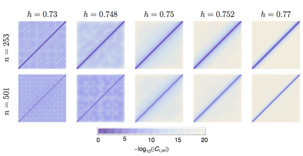
First, we use efficient prescription (43) to compute correlation matrices at non-equilibrium conditions βL=0.3βR=5.2subscript𝛽L0.3subscript𝛽R5.2\beta_{\rm L}=0.3\neq\beta_{\rm R}=5.2 and plot them for two different system sizes and five different values of hh around hcsubscriptch_{\rm c} in figure 1. Results look qualitatively identical to those for the Lindblad driving, even for other quantities that were investigated numerically in detail in [14].
Refer to caption
Figure 1: Correlation matrices Cl,msubscript𝐶𝑙𝑚C_{l,m}, l𝑙l horizontal axis (left to right), m𝑚m vertical axis (bottom to top), of the non-equilibrium thermal Redfield model of an open XY chain for γ=0.5𝛾0.5\gamma=0.5 and different field strength hh indicated at the figures (note that hc=0.75subscriptc0.75h_{\rm c}=0.75) and two diffetrent system sizes n𝑛n (indicated). Bath parameters are specified in the text.
Refer to caption
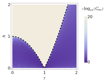
Figure 2: Phase diagram for the non-equilibrium thermal Redfield model of an open XY chain. We plot the residual correlator Cressubscript𝐶resC_{\rm res} against the bulk parameters γ𝛾\gamma, hh. The system size is fixed to n=100𝑛100n=100 and bath parameters are specified in the text.

For example, in figure 2 we plot the phase diagram of the residual correlator Cres=l,m|lm|>n/2|Cl,m|/l,m|lm|>n/21subscript𝐶ressuperscriptsubscript𝑙𝑚𝑙𝑚𝑛2subscript𝐶𝑙𝑚superscriptsubscript𝑙𝑚𝑙𝑚𝑛21C_{\rm res}=\sum_{l,m}^{|l-m|>n/2}|C_{l,m}|/\sum_{l,m}^{|l-m|>n/2}1, which also reveals possible criticality in the region of a large anisotropy γ>1𝛾1\gamma>1 previously not discussed. We note that size dependence of the residual magnetic correlator Cressubscript𝐶resC_{\rm res} shows a very characteristic behaviour: namely

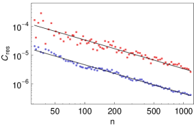
Cressubscript𝐶res\displaystyle C_{\rm res} proportional-to\displaystyle\propto exp(ηn)withη>0for|h|>hcorh=0formulae-sequence𝜂𝑛with𝜂0forsubscriptcor0\displaystyle\exp(-\eta n)\;{\rm with}\;\eta>0\quad{\rm for}\quad|h|>h_{\rm c}\;{\rm or}\;h=0 (64)
Cressubscript𝐶res\displaystyle C_{\rm res} proportional-to\displaystyle\propto 1/nfor0<|h|<hc1𝑛for0subscriptc\displaystyle 1/n\qquad\qquad\qquad\qquad\,{\rm for}\quad 0<|h|<h_{\rm c} (65)

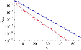
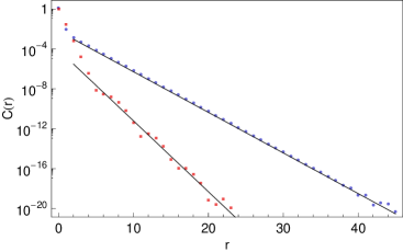
Thus we shall refer to the regime with 0<|h|<hc0subscriptc0<|h|<h_{\rm c} as long range magnetic correlation (LRMC) phase666Note, interestingly, that unlike for the local Lindblad driving[14] the XX line γ=0𝛾0\gamma=0, 0<|h|<1010<|h|<1, also exhibits long range magnetic correlations for the thermal Redfield driving., the regime with |h|>hcsubscriptc|h|>h_{\rm c}, or h=00h=0, as non-LRMC phase, and the regime with |h|=hcsubscriptc|h|=h_{\rm c} as critical. Scaling (64,65) is illustrated in figure 3. Exponential decay of the Cres(n)subscript𝐶res𝑛C_{\rm res}(n) in non-LRMC phase (64) is consistent with the exponential decay of 2-point correlator with the distance between sites C(r)=ji=rCi,j/ji=r1exp(ξr)𝐶𝑟subscript𝑗𝑖𝑟subscript𝐶𝑖𝑗subscript𝑗𝑖𝑟1similar-to𝜉𝑟C(r)=\sum_{j-i=r}C_{i,j}/\sum_{j-i=r}1\sim\exp(-\xi r), as can be qualitatively noted already in the figure 1. However, we demonstrate in figure 4 that the exponents ξ𝜉\xi could in principle be very different between the Redfield and local Lindblad models. Futhermore, as for the Linbdlad model the exponents ξ𝜉\xi and η𝜂\eta [of (64)] appear to be equal, for the Redfield model they don’t seem to be simply related. Analytical estimation of these exponents present a challenge for future theoretical work.

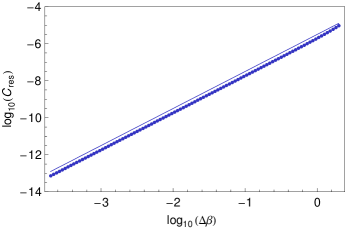
However, we note that with the thermal driving with Redfield dissipators, the long-range-magnetic order disappears when the temperatures of the baths become equal, βL=βRsubscript𝛽Lsubscript𝛽R\beta_{\rm L}=\beta_{\rm R}, and there we recover, consistently, all the properties of the thermal state [15] which are most easily numerically reproduced by the method of Ref.[16] , i.e. fast decay of correlations for any hh and absence of long-range order. For example, it is interesting to note how the residual correlator Cressubscript𝐶resC_{\rm res} (for large n𝑛n in the LRMC phase) decreases as a function of the difference of inverse temperatures Δβ=βRβLΔ𝛽subscript𝛽Rsubscript𝛽L\Delta\beta=\beta_{\rm R}-\beta_{\rm L}, namely numerics of figure 5 suggests clearly that Cres(Δβ)2.proportional-tosubscript𝐶ressuperscriptΔ𝛽2C_{\rm res}\propto(\Delta\beta)^{2}.
Refer to caption
Refer to caption
Figure 3: Residual correlator Cressubscript𝐶resC_{\rm res} as a function of the system size n𝑛n for the LRMC phase (γ=0.5,h=0.2formulae-sequence𝛾0.50.2\gamma=0.5,h=0.2, left plot) and non-LRMC phase (γ=0.5,h=0.9formulae-sequence𝛾0.50.9\gamma=0.5,h=0.9, right plot), where we compare the non-equilibrium thermal Redfield model (red squares) and the non-equilibrum Lindblad model (blue circles) with bath parameters as specified in the text. The thin lines indicated the suggested behavior 1/n1𝑛1/n (on the left) and exp(ηn)𝜂𝑛\exp(-\eta n) on the right (with the numerical best fit η=1.192𝜂1.192\eta=1.192 for the Redfield model and η=0.937𝜂0.937\eta=0.937 for the Lindblad model).
Refer to caption
Figure 4: Comparing the decay of the 2-point spin-spin correlator C(r)=ji=rCi,j/ji=r1exp(ξr)𝐶𝑟subscript𝑗𝑖𝑟subscript𝐶𝑖𝑗subscript𝑗𝑖𝑟1similar-to𝜉𝑟C(r)=\sum_{j-i=r}C_{i,j}/\sum_{j-i=r}1\sim\exp(-\xi r) between the non-equlibrium thermal Redfield model (red squares) and non-equilibrium Lindblad model (blue circles) for the same values of bulk parameters in the non-LRMC phase (h=1.05,γ=0.2,n=200formulae-sequence1.05formulae-sequence𝛾0.2𝑛200h=1.05,\gamma=0.2,n=200) and bath parameters specified in the text. The thin lines indicate suggested exponential decays exp(ξr)proportional-toabsent𝜉𝑟\propto\exp(-\xi r) with the exponents ξ=1.635𝜉1.635\xi=1.635 (fitting the Redfield model) and ξ=0.937𝜉0.937\xi=0.937 (fitting the Lindblad model).
Refer to caption
Figure 5: Residual correlation Cressubscript𝐶resC_{\rm res} versus the (inverse) temperature drop ΔβΔ𝛽\Delta\beta between the left and the right bath, βL=2Δβ/2subscript𝛽𝐿2Δ𝛽2\beta_{L}=2-\Delta\beta/2, βR=2+Δβ/2subscript𝛽𝑅2Δ𝛽2\beta_{R}=2+\Delta\beta/2, for the non-equilibrium thermal Redfield model of an open XY chain in LRMC phase (γ=0.5,h=0.3formulae-sequence𝛾0.50.3\gamma=0.5,h=0.3), system size n=100𝑛100n=100, and the bath parameters specified in the text. The thin line indicated suggested |Δβ|2superscriptΔ𝛽2|\Delta\beta|^{2} behavior.

Heuristic explanation of this non-equilibrium phase transition is rather straightforward [14], however its exact proof and also the quantitative dependence of the decay exponent η(γ,h)𝜂𝛾\eta(\gamma,h) are still lacking. We note that the transition point h=hcsubscriptch=h_{\rm c} is characterized by a simple property of the XY spin chain quasiparticle dispersion relation

ω(q)=(cosqh)2+γ2sin2q,𝜔𝑞superscript𝑞2superscript𝛾2superscript2𝑞\omega(q)=\sqrt{(\cos q-h)^{2}+\gamma^{2}\sin^{2}q}\ , (66)

where ϵj=ω(2πj/n)subscriptitalic-ϵ𝑗𝜔2𝜋𝑗𝑛\epsilon_{j}=\omega(2\pi j/n) would be exactly the (positive) eigenvalues of matrix 𝐇𝐇{\mathbf{H}} if periodic boundary conditions would be imposed on the closed system. Namely, in non-LRMC phase |h|>hcsubscriptc|h|>h_{\rm c} there exist only a single pair of trivial stationary points q=0,πsuperscript𝑞0𝜋q^{*}=0,\pi, whereas in LRMC phase |h|<hcsubscriptc|h|<h_{\rm c} there exist another pair of nontrivial stationary points ±q0,πplus-or-minussuperscript𝑞0𝜋\pm q^{*}\neq 0,\pi, dω/dq|q=q=0evaluated-atd𝜔d𝑞𝑞superscript𝑞0{\rm d}\omega/{\rm d}q|_{q=q^{*}}=0, which introduces a new non-trivial length scale 1/q1superscript𝑞1/q^{*} which determines typical sizes of correlated regions in the matrix Cl,msubscript𝐶𝑙𝑚C_{l,m} (see figure 1). Therefore this simple non-equilibrium quasi-particle picture predicts mean-field critical exponent 1/q|hch|1/2similar-to1superscript𝑞superscriptsubscriptc121/q^{*}\sim|h_{\rm c}-h|^{-1/2} as hhcsubscriptch\uparrow h_{\rm c} (confirmed in Ref.[14]).

Refer to caption
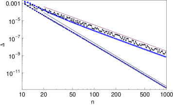
Figure 6: Liouvilllean spectral gap ΔΔ\Delta for the non-equilibrum thermal Redfield model of an open XY chain. We plot three different cases with: γ=0.5𝛾0.5\gamma=0.5, h=0.8>hc0.8subscriptch=0.8>h_{\rm c} (non-LRMC phase, light blue circles), γ=0.5𝛾0.5\gamma=0.5, h=0.75=hc0.75subscriptch=0.75=h_{\rm c} (critical regime, dark blue squares), γ=0.5𝛾0.5\gamma=0.5, h=0.3<hc0.3subscriptch=0.3<h_{\rm c} (LRMC phase, black diamonds), whereas the bath parameters are specified in the text. Suggested power law decays n3superscript𝑛3n^{-3} and n5superscript𝑛5n^{-5} are indicated with thin lines.

The non-equilibrium quantum phase transition can also be characterized by the scaling of the Liouvillean spectral gap Δ(n)Δ𝑛\Delta(n), namely in the critical regime one expects a qualitative increase in the relaxation time 1/Δ1Δ1/\Delta to NESS. Numerical results (see figrure 6) suggest the spectral gap of the Liouvillean remains like in the local Lindblad case [11]

Δn3forhhc,Δn5forh=hc,formulae-sequenceproportional-toΔsuperscript𝑛3forsubscriptcproportional-toΔsuperscript𝑛5forsubscriptc\Delta\propto n^{-3}\;{\rm for}\;h\neq h_{\rm c},\qquad\Delta\propto n^{-5}\;{\rm for}\;h=h_{\rm c}, (67)

although we are at the moment unable to prove this conjecture. Also note slight fluctuations of Δ(n)Δ𝑛\Delta(n) in the LRMC phase as opposed to a smooth power law in the non-LRMC phase.

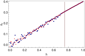
Long range correlations for |h|<hcsubscriptc|h|<h_{\rm c} naturally imply sensitivity of NESS to tiny variations in system’s parameters. For example, one may expect also that local observables in NESS will be then sensitive functions of the bath-driving or even bulk parameters, such as the magnetic field hh. In figure 7 we plot local magnetization in the center of the chain sz=σn/2zNESSsubscript𝑠zsubscriptdelimited-⟨⟩subscriptsuperscript𝜎z𝑛2NESSs_{\rm z}={\langle\sigma^{\rm z}_{n/2}\rangle}_{\rm NESS} versus the field strength hh. Indeed, we notice that for |h|>hcsubscriptc|h|>h_{\rm c}, sz(h)subscript𝑠zs_{\rm z}(h) is a smooth function wheres for |h|<hcsubscriptc|h|<h_{\rm c}, sz(h)subscript𝑠zs_{\rm z}(h) becomes rapidly oscillating or better to say, fluctuating, function. Even though the amplitude of these oscillations decreases with n𝑛n, the scale of hh on which sz(h)subscript𝑠zs_{\rm z}(h) fluctuates decreases with n𝑛n even much faster, so we predict that in the thermodynamic limit n𝑛n\to\infty, in LRMC phase the local susceptibility dsz/dhdsubscript𝑠zd{\rm d}s_{\rm z}/{\rm d}h would be ill defined. In summary, LRMC phase can be characterized by hypersensitivity of NESS to external parameters.
Refer to caption
Figure 7: Hypersensitivity of NESS to magnetic field strength hh. We plot local magnetization sz(h)=σn/2zNESSsubscript𝑠zsubscriptdelimited-⟨⟩subscriptsuperscript𝜎z𝑛2NESSs_{\rm z}(h)={\langle\sigma^{\rm z}_{n/2}\rangle}_{\rm NESS} for the non-equilibrium thermal Redfield model of open XY chain with γ=0.5𝛾0.5\gamma=0.5 and bath parameters as written in the text. Big blue (small red) circles represent data for n=50𝑛50n=50 (n=100𝑛100n=100), whereas vertical line denotes the critical value h=hcsubscriptch=h_{\rm c}.

4.2 Heat transport and entropies

An important non-equilibrium physical effect which one can investigate more deeply in an open XY chain is the heat transport, which has been recently intensively studied in quantum spin chains, see e.g.[17, 18, 19, 20, 21] or [22] for a recent review on the topic.

Writing the Hamiltonian (54) in the bulk as a sum H=mHm𝐻subscript𝑚subscript𝐻𝑚H=\sum_{m}H_{m} with a two body energy density operator

Hmsubscript𝐻𝑚\displaystyle H_{m} =\displaystyle= i1+γ2w2mw2m+1+i1γ2w2m1w2m+2i1𝛾2subscript𝑤2𝑚subscript𝑤2𝑚1i1𝛾2subscript𝑤2𝑚1subscript𝑤2𝑚2\displaystyle-{\rm i}\frac{1+\gamma}{2}w_{2m}w_{2m+1}+{\rm i}\frac{1-\gamma}{2}w_{2m-1}w_{2m+2} (68)
ihm2w2m1w2mihm+12w2m+1w2m+2,isubscript𝑚2subscript𝑤2𝑚1subscript𝑤2𝑚isubscript𝑚12subscript𝑤2𝑚1subscript𝑤2𝑚2\displaystyle-{\rm i}\frac{h_{m}}{2}w_{2m-1}w_{2m}-{\rm i}\frac{h_{m+1}}{2}w_{2m+1}w_{2m+2},

one can derive the local energy current

Qmsubscript𝑄𝑚\displaystyle Q_{m} =\displaystyle= i[Hm,Hm+1]isubscript𝐻𝑚subscript𝐻𝑚1\displaystyle{\rm i}[H_{m},H_{m+1}]
=\displaystyle= i(1γ2)(w2m1w2m+3+w2mw2m+4)i1superscript𝛾2subscript𝑤2𝑚1subscript𝑤2𝑚3subscript𝑤2𝑚subscript𝑤2𝑚4\displaystyle{\rm i}(1-\gamma^{2})(w_{2m-1}w_{2m+3}+w_{2m}w_{2m+4})
\displaystyle- 2ih(1γ)(w2m1w2m+1+w2m+2w2m+4)2i1𝛾subscript𝑤2𝑚1subscript𝑤2𝑚1subscript𝑤2𝑚2subscript𝑤2𝑚4\displaystyle 2{\rm i}h(1-\gamma)(w_{2m-1}w_{2m+1}+w_{2m+2}w_{2m+4})
\displaystyle- 2ih(1+γ)(w2mw2m+2+w2m+1w2m+3),2i1𝛾subscript𝑤2𝑚subscript𝑤2𝑚2subscript𝑤2𝑚1subscript𝑤2𝑚3\displaystyle 2{\rm i}h(1+\gamma)(w_{2m}w_{2m+2}+w_{2m+1}w_{2m+3}),

which, by construction, satisfies the continuity equation

(d/dt)Hm=i[H,Hm]+trHm𝒟^ρ(t)=Qm+Qm1.dd𝑡delimited-⟨⟩subscript𝐻𝑚delimited-⟨⟩i𝐻subscript𝐻𝑚trsubscript𝐻𝑚^𝒟𝜌𝑡delimited-⟨⟩subscript𝑄𝑚delimited-⟨⟩subscript𝑄𝑚1({\rm d}/{\rm d}t){\langle H_{m}\rangle}={\langle{\rm i}[H,H_{m}]\rangle}+{\,{\rm tr}\,}H_{m}\hat{\cal D}\rho(t)=-{\langle Q_{m}\rangle}+{\langle Q_{m-1}\rangle}. (70)

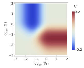
The two terms between the two equality signs above correspond to the unitary and dissipative term in the master equation (3). The unitary term has been already transformed to a simple expectation value using cyclicity of the trace trx[y,z]try[z,x]tr𝑥𝑦𝑧tr𝑦𝑧𝑥{\,{\rm tr}\,}x[y,z]\equiv{\,{\rm tr}\,}y[z,x], while the dissipative term can be further shown to vanish in the bulk 2mn22𝑚𝑛22\leq m\leq n-2 by excercising the cyclicity of the trace again and transforming the integrand of (4) to terms of the form trX~μ(τ)ρ[Xν,Hm]0trsubscript~𝑋𝜇𝜏𝜌subscript𝑋𝜈subscript𝐻𝑚0{\,{\rm tr}\,}\tilde{X}_{\mu}(-\tau)\rho[X_{\nu},H_{m}]\equiv 0. The RHS expression of eq. (70) then follows from the nearest-neighbour locality of the Hamiltonian. Therefore, in NESS the expectation value of the current QmNESSsubscriptdelimited-⟨⟩subscript𝑄𝑚NESS{\langle Q_{m}\rangle}_{\rm NESS} should be independent of the position m𝑚m. By looking at the dependence of the steady-state current on the system size we clearly find ballistic transport, namely QmNESS=𝒪(n0)subscriptdelimited-⟨⟩subscript𝑄𝑚NESS𝒪superscript𝑛0{\langle Q_{m}\rangle}_{\rm NESS}={\cal O}(n^{0}), irrespectively of the temperature differences between the baths and bulk parameters of the model (i.e. whether being in the LRMC phase, non-LRMC phase, or critical). However, we find very interesting dependence of the heat current on the temperature driving, i.e. on the two temperatures of the thermal baths. In figure 8 we plot QmNESSsubscriptdelimited-⟨⟩subscript𝑄𝑚NESS{\langle Q_{m}\rangle}_{\rm NESS} versus βLsubscript𝛽L\beta_{\rm L} and βRsubscript𝛽R\beta_{\rm R} and find a maximum of the current for intermediate driving, namely when one of the temperatures is less than one 1/βL<11subscript𝛽L11/\beta_{\rm L}<1 and the other temperature is about 1/βR201subscript𝛽R201/\beta_{\rm R}\approx 20. This is a clear signature of negative differential heat conductance which could perhaps be related to similar far-from-equilibroum effects recently observed in spin and charge transport [23].

This behavior can be nicely characterized by computing the Gibbs entropy of NESS. Since NESS is completely characterized by quadratic correlations wjwkNESSsubscriptdelimited-⟨⟩subscript𝑤𝑗subscript𝑤𝑘NESS{\langle w_{j}w_{k}\rangle}_{\rm NESS} and the Wick theorem, one can adopt the recipe which has been proposed in Ref.[24] for computing block entropies (or entanglement entropies) applied to the entire lattice. In fact, taking an arbitrary block region A{1,,n}𝐴1𝑛A\subseteq\{1,\ldots,n\}, one can compute Von Neumann entropy SA(ρ)=trAρAlog2ρAsubscript𝑆𝐴𝜌subscripttr𝐴subscript𝜌𝐴subscript2subscript𝜌𝐴S_{A}(\rho)=-{\rm tr}_{A}\rho_{A}\log_{2}\rho_{A} (in base 222), where ρA=trA¯ρsubscript𝜌𝐴subscripttr¯𝐴𝜌\rho_{A}={\rm tr}_{\bar{A}}\rho is a reduced density matrix and A¯¯𝐴\bar{A} denotes the complement of A𝐴A, as

SA=j=1#(A)H2((1+νj)/2)withH2(x):=xlog2x(1x)log2xsubscript𝑆𝐴superscriptsubscript𝑗1#𝐴subscript𝐻21subscript𝜈𝑗2withsubscript𝐻2𝑥assign𝑥subscript2𝑥1𝑥subscript2𝑥S_{A}=\sum_{j=1}^{\#(A)}H_{2}((1+\nu_{j})/2)\;\;{\rm with}\;\;H_{2}(x):=-x\log_{2}x-(1-x)\log_{2}x (71)

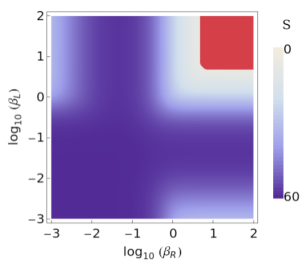
and ±iνjplus-or-minusisubscript𝜈𝑗\pm{\rm i}\nu_{j} are the eigenvalues of the 2#(A)×2#(A)2#𝐴2#𝐴2\#(A)\times 2\#(A) part of the correlation matrix Bj,ksubscript𝐵𝑗𝑘B_{j,k} defined by wjwkNESS=:δj,k+iBj,k{\langle w_{j}w_{k}\rangle}_{\rm NESS}=:\delta_{j,k}+{\rm i}B_{j,k}, restricted to Majorana operators wj,wksubscript𝑤𝑗subscript𝑤𝑘w_{j},w_{k} corresponding to spins from the block A𝐴A. The same general procedure has been applied to thermal (Gibbs) states in Ref.[16]. When taking the maximal block A={1,,n}𝐴1𝑛A=\{1,\ldots,n\} we obtain exactly the standard Gibbs entropy of NESS. In figure 9 we plot the Gibbs entropy S{1,,n}subscript𝑆1𝑛S_{\{1,\ldots,n\}} as a function of two bath temperatures and show that, quite remarkably, the regions of large (maximal) heat current correspond to regions of large (locally maximal) Gibbs entropy. This is not unexpected as the product of the heat current and the inverse temperature difference ΔβΔ𝛽\Delta\beta may be understood as the entropy production rate.

Calculation of Gibbs entropy of NESS provides also a nice way of controlling the positivity of NESS as a density matrix, since this is by no means guaranteed by the Redfield master equation. Indeed we find that for very small temperatures (large β𝛽\beta’s), or for very strong bath coupling λ𝜆\lambda, the positivity of NESS might be slightly violated (red region in figure 9), namely some of the correlation matrix eigenvalues νjsubscript𝜈𝑗\nu_{j} become slightly larger than 111 (but in our numerical experience never by more than 107superscript10710^{-7} or so).

Refer to caption
Figure 8: NESS expectation value of the heat current QmNESSsubscriptdelimited-⟨⟩subscript𝑄𝑚NESS{\langle Q_{m}\rangle}_{\rm NESS} versus two inverse temperatures βLsubscript𝛽L\beta_{\rm L} and βRsubscript𝛽R\beta_{\rm R} for the non-equilibrium thermal Redfield model of an open XY chain with γ=0.5,h=0.9formulae-sequence𝛾0.50.9\gamma=0.5,h=0.9, sistem size n=53𝑛53n=53, and bath parameters given in the text. Note that the ‘shoulders’ of maxima, around βL0.05,βR>1formulae-sequencesubscript𝛽L0.05subscript𝛽R1\beta_{\rm L}\approx 0.05,\beta_{\rm R}>1, and with LL{\rm L} and RR{\rm R} exchanged, could be interpreted as negative differential heat conductance.

We can use the concept of block entropy of NESS to further characterize the non-equilibrium phase transition. For example, we may compute the total (quantum plus classical) correlations between two halves of the spin chain in NESS as given by quantum mutual information QMI I(n)=S{1,,n/2}+S{n/2+1,,n}S{1,,n}𝐼𝑛subscript𝑆1𝑛2subscript𝑆𝑛21𝑛subscript𝑆1𝑛I(n)=S_{\{1,\ldots,n/2\}}+S_{\{n/2+1,\ldots,n\}}-S_{\{1,\ldots,n\}}.

Refer to caption
Figure 9: Gibbs entropy of NESS versus two inverse temperatures βLsubscript𝛽L\beta_{\rm L} and βRsubscript𝛽R\beta_{\rm R} for the same parameters as in the figure 8. Note that in the red region (of both large inverse temperatures), NESS is no longer a density matrix (at least one of the eigenvalues becomes slightly negative) hence the Gibbs entropy is strictly no longer defined there.

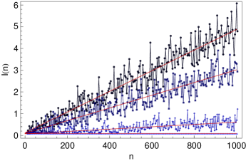
Interestingly, we find (see figure 10) that QMI saturates I(n)=𝒪(n0)𝐼𝑛𝒪superscript𝑛0I(n)={\cal O}(n^{0}) in the non-LRMC phase (for |h|>hcsubscriptc|h|>h_{\rm c}), whereas in LRMC phase (for 0<|h|<hc0subscriptc0<|h|<h_{\rm c}) QMI becomes extensive I(n)=𝒪(n)𝐼𝑛𝒪𝑛I(n)={\cal O}(n) indicating a drastic enhancement of correlations in NESS. This is again very similar to the behaviour of operator space entanglement entropy (OSEE) (analized for the Lindblad model in [14]), so one may extend the relationship between QMI and OSEE which has been conjectured for thermal states in Ref.[16] to NESS.
Refer to caption
Figure 10: Another manifestation of the non-equilibrium phase transition: Quantum mutual information (QMI) of NESS for non-equlibrium thermal Redfield model of open XY spin chain. The bulk parameters are γ=0.5𝛾0.5\gamma=0.5 and h=0.9>hc=0.750.9subscriptc0.75h=0.9>h_{\rm c}=0.75 (lightest blue, saturated curve), h=0.70.7h=0.7, h=0.50.5h=0.5 and h=0.30.3h=0.3 (from lighter to darker blue curves). Thin red lines indicated the linear growth of QMI for h<hcsubscriptch<h_{\rm c}.

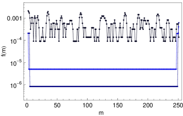
In the context of energy transport it is interesting to look at the energy density profiles in NESS. In figure 11 we plot the relative spatial fluctuation of the energy density f(m)=|HmNESSH¯|/|H¯|𝑓𝑚subscriptdelimited-⟨⟩subscript𝐻𝑚NESS¯𝐻¯𝐻f(m)=|{\langle H_{m}\rangle}_{\rm NESS}-\bar{H}|/|\bar{H}| where H¯=(n3)1m=2n2HmNESS¯𝐻superscript𝑛31superscriptsubscript𝑚2𝑛2subscriptdelimited-⟨⟩subscript𝐻𝑚NESS\bar{H}=(n-3)^{-1}\sum_{m=2}^{n-2}{\langle H_{m}\rangle}_{\rm NESS} is the averaged energy density. Quite strikingly, we observe a big variation of f(m)𝑓𝑚f(m) from site to site for LRMC phase and very smooth (non-fluctuating) behaviour for the non-LRMC phase which is characterized with a bulk-constant f(m)𝑓𝑚f(m) which is exponentially small in n𝑛n. This behaviour can again be considered as a manifestation of hypersensitivity of NESS and LRMC.
Refer to caption
Figure 11: Another manifestation of non-equilibrium phase transition: positional fluctuations in energy density in NESS of non-equilirbium thermal Redfield model of open XY chain. We plot the relative fluctuation f(m)=|HmNESSH¯|/|H¯|𝑓𝑚subscriptdelimited-⟨⟩subscript𝐻𝑚NESS¯𝐻¯𝐻f(m)=|{\langle H_{m}\rangle}_{\rm NESS}-\bar{H}|/|\bar{H}| where H¯¯𝐻\bar{H} is the bulk average of energy density HmNESSsubscriptdelimited-⟨⟩subscript𝐻𝑚NESS{\langle H_{m}\rangle}_{\rm NESS}. Three curves correspond to γ=0.5𝛾0.5\gamma=0.5 and h=0.7<hc0.7subscriptch=0.7<h_{\rm c} (black curve), h=0.75=hc0.75subscriptch=0.75=h_{\rm c} (dark blue curve) and h=0.8>hc0.8subscriptch=0.8>h_{\rm c} (light blue curve), while the system size is n=253𝑛253n=253.
Refer to caption
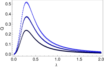
Figure 12: NESS expectation value of the heat current QmNESSsubscriptdelimited-⟨⟩subscript𝑄𝑚NESS{\langle Q_{m}\rangle}_{\rm NESS} versus the coupling strength λ𝜆\lambda for the non-equilibrium thermal Redfield model of an open XY chain with h=0.5<hc0.5subscriptch=0.5<h_{\rm c} (black curve), h=0.75=hc0.75subscriptch=0.75=h_{\rm c} (dark blue curve) and h=1.0>hc1.0subscriptch=1.0>h_{\rm c} (light blue curve), system size n=200𝑛200n=200 and other bath parameters as given in the text. Note that the full line gives numerically excellent fit to the Karevski and Platini formula [25] Qm=aλ2/(b+λ4)delimited-⟨⟩subscript𝑄𝑚𝑎superscript𝜆2𝑏superscript𝜆4{\langle Q_{m}\rangle}=a\lambda^{2}/(b+\lambda^{4}) for best fitted parameters a=0.040,b=0.0070formulae-sequence𝑎0.040𝑏0.0070a=0.040,b=0.0070, a=0.066,b=0.0076formulae-sequence𝑎0.066𝑏0.0076a=0.066,b=0.0076, and a=0.088,b=0.0071formulae-sequence𝑎0.088𝑏0.0071a=0.088,b=0.0071 for the three cases of h=0.5,0.75,1.00.50.751.0h=0.5,0.75,1.0, respectively.

At last we check the dependence of the heat current QmNESSsubscriptdelimited-⟨⟩subscript𝑄𝑚NESS{\langle Q_{m}\rangle}_{\rm NESS} on the system-bath coupling strength λ𝜆\lambda. It was recently reported by Karevski and Platini [25] that the spin current Jmsubscript𝐽𝑚J_{m} in the local Lindblad model of an open isotropic XX chain γ=0𝛾0\gamma=0 has a non-monotonic dependence on λ𝜆\lambda which can be universally described by a formula JmNESS=aλ2/(b+λ4)subscriptdelimited-⟨⟩subscript𝐽𝑚NESSsuperscript𝑎superscript𝜆2superscript𝑏superscript𝜆4{\langle J_{m}\rangle}_{\rm NESS}=a^{\prime}\lambda^{2}/(b^{\prime}+\lambda^{4}) where a,bsuperscript𝑎superscript𝑏a^{\prime},b^{\prime} are some constants. For the anisotropic XY model and general non-equilibrium thermal Redfield driving we are unable to derive an exact analytic result, however our numerical simulations suggest a very similar behaviour for the heat current

QmNESSaλ2/(b+λ4),subscriptdelimited-⟨⟩subscript𝑄𝑚NESS𝑎superscript𝜆2𝑏superscript𝜆4{\langle Q_{m}\rangle}_{\rm NESS}\approx a\lambda^{2}/(b+\lambda^{4}), (72)

where a,b𝑎𝑏a,b are again some constants which may depend on all system’s parameters except λ𝜆\lambda. This is particulary interesting as in the anisotropic XY model the spin current is not even well defined as there is no corresponding conservation law. This behaviour is demonstrated in figure 12 where on may also notice small but detectable deviations between numerics and the best fit to (72). We note that the error of the fit does not decrease but is roughly constant when we increase the system size n𝑛n.

5 Discussion

The purpose of the present paper was three-fold. Firstly, we have outlined a general method for exact treatment of quadratic many-body Markovian master equations. Our formalism, which rests upon treating density operators as elements of a suitable operator Fock space (or Liouville-Fock space) is quite flexible and allows for explicit solution of static and time-dependent quantum many-body Liouvillean problems, for example computation of arbitrary physical obsevables in the non-equilibrium steady state, decay rates of approach to the steady state, or even time-evolution of the density matrix of externally forced systems described by explicitly time-dependent Liouvilleans, all with polynomial computation complexity in number of particles (fermionic degrees of freedom).

Secondly, we have analyzed in detail the Redfield model of thermal baths within our framework. In spite of the fact that the Redfield model does not define a proper dynamical semigroup, namely it is not guaranteed to preserve positivity of the density operator, we have confirmed that steady states typically correspond to proper (positive) density operators. Tiny deviations from positivity have only been observed in some test cases for very small temperatures or very large couplings to the baths (which anyway violate weak coupling assumption). Furthermore, we have shown that coupling the central system with several thermal baths of the Redfield type at different temperatures produces physically interesting non-equilibrium steady states, for example such states which carry non-vanishing heat current. We wish to stress this physically obvious but mathematically delicate point with a particular care, as we have found a qualitatively different result for Lindblad-Davies dissipators which generate proper dynamical semigroups and satisfy detailed balance condition with respect to Gibbs states [26, 5]. Namely when we constructed a Lindblad-Davies dissipator with respect to two baths with two different temperatures coupled to two ends of the system (spin chain), we have found that the resulting steady state (fixed point of the Liouvillean dynamics) is simply some convex combination of two Gibbs states corresponding to the bath temperatues, and as such has always zero heat current and cannot represent physical steady state. This implies that the secular approximation (sometimes called the rotating wave approximation) which is the one-step from the Redfield to the Lindblad-Davies bath model prohibits the emergence of the physical out-of-equilibrium steady states with currents, therefore the seemingly harmless rapidly oscillating terms in the Redfield dissipator may be absolutely essential for non-equilibrium physics. Thus we conjecture that the thermal Redfield model is somehow a minimal mathematical model which can describe non-equilibrium thermal driving of a (non-self-thermalizing, e.g. integrable) open quantum system.

Thirdly, we have applied our theory to analyze non-equilibrium quanutm phase transition and heat transport in an open XY spin 1/2 chain. We have carefully compared numerical results for the non-equilibrium thermal Redfield model and the local Lindblad model, which has been discussed before [11, 14]. We have found that the phase diagram of the non-equilibrium XY model is insensitive to the theory with which we describe the baths, and the differences were only quantitative. In particular we wish to stress that thermally driven heat current in the XY chains exhibits non-monotonic dependence on the temperature difference which may be interpreted as negative differential heat conductance. We believe that our numerical results on non-equilibrium open XY chain provide a strong motivation for further analytical work. In particular, we believe that the block-tridiagonal plus block-bordered structure of the Liouvillean structure matrix (58,59) could be explored in combination with the non-equilibrium Green function formula for the observables (44,45) to yield explicit asymptotic results for large n𝑛n.

Note added: Formally quite similar approach to non-equilibrium quasi-particles has recently been developed independently by Kosov [27].

We acknowledge financial support by the Programme P1-0044, and the Grant J1-2208, of the Slovenian Research Agency (ARRS).

References

References

  • [1] H. Araki and E. Barouch, J. Stat. Phys. 31, 327 (1983);
    H. Araki, Publ. RIMS Kyoto Univ. 20, 277 (1984).
  • [2] D. Ruelle, J. Stat. Phys. 98, 57 (2000).
  • [3] V. Jakšič and C.-A. Pillet, J. Stat. Phys. 108, 787 (2002); Commun. Math. Phys. 226, 131 (2002);
    W. Aschbacher, V. Jakšič, Y. Pautrat and C.-A. Pillet, Inroduction to non-equilibrium quantum statistical mechanics, in Open Quantum Systems III. Recent Developments Lecture Notes in Mathematics, 1882 (2006), 1-66.
  • [4] H.-P. Breuer and F. Petruccione, The Theory of Open Quantum Systems (Oxford University Press, Oxford 2002).
  • [5] R. Alicki and K. Lendi, Quantum dynamical semigroups and applications (Springer, 2007).
  • [6] H. Wichterich, M. J. Herich, H. P. Breuer, J. Gemmer and M. Michel, Phys. Rev. E, 76 031115 (2007).
  • [7] I. Sinaysky, F. Petruccione and D. Burgarth, Phys. Rev. A 78, 062301 (2008).
  • [8] M. Ban, J. Mod. Opt. 56, 577 (2009).
  • [9] S. R. White, Phys. Rev. Lett. 69, 2863 (1992);
    U. Schollwöck, Rev. Mod. Phys. 77, 259 (2005);
    G. Vidal, Phys. Rev. Lett. 91, 147902 (2003); ibid. 93, 040502 (2004).
  • [10] T. Prosen and M. Žnidarič, J. Stat. Mech, P02035 (2009).
  • [11] T. Prosen, New J. Phys. 10, 040326 (2008).
  • [12] I. Pižorn, “Entanglement and Quantum Critical Phenomena: Operator Spaces and Random Matrix Theory”, PhD Thesis, University of Ljubljana.
  • [13] T. Prosen and I. Pižorn, to be published (2009).
  • [14] T. Prosen and I. Pižorn, Phys. Rev. Lett. 101, 105701 (2008).
  • [15] E. Barouch, B. M. McCoy, Phys. Rev. A 3, 786 (1971); ibid 2140 (1971).
  • [16] M. Žnidarič, T. Prosen and I. Pižorn, Phys. Rev. A 78, 022103 (2008).
  • [17] K. Saito, S. Takesue and S. Miyashita, Phys. Rev. E 61, 2397 (2000);
    K. Saito, Europhys. Lett. 61, 34 (2003).
  • [18] F. Heidrich-Meisner, A. Honecker, D. C. Cabra, and W. Brenig, Phys. Rev. B 66, 140406 (2002);
    F. Heidrich-Meisner, A. Honecker, W. Brenig, Phys. Rev. B 71, 184415 (2005).
  • [19] C. Mejia-Monasterio, T. Prosen and G. Casati, Europhys. Lett. 72, 520 (2005).
  • [20] M. Michel, M. Hartmann, J. Gemmer and G. Mahler, Eur. Phys. J. B. 34, 325 (2003);
    M. Michel, G. Mahler and J. Gemmer, Phys. Rev. Lett. 95, 180602 (2005);
    J. Gemmer, R. Steinigeweg and M. Michel, Phys. Rev. B 73, 104302 (2006);
    R. Steinigeweg, M. Ogiewa, and J. Gemmer, Europhys. Lett. 87, 10002 (2009).
  • [21] L. Arrachea, G. S. Lozano, and A. A. Aligia, Phys. Rev. B 80, 014425 (2009).
  • [22] A. Dhar, Adv. Phys. 57, 457 (2008).
  • [23] G. Benenti, G. Casati, T. Prosen and D. Rossini, Europhys. Lett. 85, 37001 (2009);
    G. Benenti, G. Casati, T. Prosen, D. Rossini and M. Žnidarič, Phys. Rev. B 80, 035110 (2009).
  • [24] G. Vidal, J. I. Latorre, E. Rico, and A. Kitaev, Phys. Rev. Lett. 90, 227902 (2003);
    J. I. Latorre, E. Rico, and G. Vidal, Quant. Inf. Comp.4, 48 (2004).
  • [25] D. Karevski and T. Platini, Phys. Rev. Lett. 102, 207207 (2009).
  • [26] E. B. Davies, Comm. Math. Phys. 39, 91 (1974);
    R. Alicki, Rep. Math. Phys. 10, 249 (1976);
    A. Kossakovski, A. Frigerio, V. Gorini, and M. Verri, Comm. Math. Phys. 57, 97 (1977);
    H. Spohn, Lett. Math. Phys. 2, 33 (1977);
    A. Frigerio, Lett. Math. Phys. 2, 79 (1977).
  • [27] D. S. Kosov, arXiv:0907.1045v1.