Stabilization and destabilization of second-order solitons against perturbations in the nonlinear Schrödinger equation.

Abstract

We consider splitting and stabilization of second-order solitons (2-soliton breathers) in a model based on the nonlinear Schrödinger equation (NLSE), which includes a small quintic term, and weak resonant nonlinearity management (NLM), i.e., time-periodic modulation of the cubic coefficient, at the frequency close to that of shape oscillations of the 2-soliton. The model applies to the light propagation in media with cubic-quintic optical nonlinearities and periodic alternation of linear loss and gain, and to BEC, with the self-focusing quintic term accounting for the weak deviation of the dynamics from one-dimensionality, while the NLM can be induced by means of the Feshbach resonance. We propose an explanation to the effect of the resonant splitting of the 2-soliton under the action of the NLM. Then, using systematic simulations and an analytical approach, we conclude that the weak quintic nonlinearity with the self-focusing sign stabilizes the 2-soliton, while the self-defocusing quintic nonlinearity accelerates its splitting. It is also shown that the quintic term with the self-defocusing/focusing sign makes the resonant response of the 2-soliton to the NLM essentially broader, in terms of the frequency.

A well-known consequence of the integrability of the one-dimensional nonlinear Schrödinger equation with the self-focusing cubic nonlinear term is that this equation gives rise to an infinite family of $N$-th order soliton solutions, in the form of periodically oscillating breathers (the oscillation period is the same for all $N\geq 2$). These solutions may be interpreted as bound states of $N$ overlapping fundamental solitons with different amplitudes. Their binding energy being exactly zero, all $N$-soliton complexes are unstable against perturbations of the initial conditions, which can split them into slowly separating constituent fundamental pulses. In this work, we aim to study the stabilization/destabilization of the $2$- (second-order) solitons by a weak additional quintic self-focusing/self-defocusing term. Various origins of such additional nonlinearity, of either sign, are known in Bose-Einstein condensates (BECs) and nonlinear optics, being within the reach of available experimental techniques. We argue that our predictions of the change in the stability of the higher-order solitons, and of a possibility to implement the precise control of the soliton dynamics by means of the quintic nonlinear term, may be realized in experiments with optical and matter-wave solitons. The analysis is performed using a combination of direct simulations and analytical approximations.

I Introduction

The control of soliton dynamics has been drawing a great deal of interest both as a fundamental problem and a topic with a vast spectrum of applications – in particular, to optics and matter waves management . It is well known that the nonlinear Schrödinger equation (NLSE), being an integrable one, supports an infinite sequence of exact higher-order soliton solutions, which may be understood as bound states of strongly overlapping fundamental solitons TheorySolitons . However, within the framework of the integrable equation, the binding energy of the exact multi-soliton complex is always equal to zero TheorySolitons , hence the higher-order solitons are unprotected (unstable) against perturbations of initial conditions, which can induce splitting into fundamental constituents. For example, the second- and third-order solitons (which are often briefly called 2-soliton and 3-soliton, respectively) readily split into sets of two and three fundamental solitons, with amplitude ratios $1:3$ and $1:3:5$.

Different approaches were proposed to stimulate the splitting and make it a real physical effect. One possibility is to introduce a specific nonlinear dissipation into the model by adding nonconservative terms to the NLSE, such as the one accounting for the intrapulse Raman scattering in optical fibers SolitonsInOC . Other physically relevant settings are those with a periodic modulation of either the group-velocity-dispersion (GVD) or nonlinearity coefficient in the NLSE, which is known as the dispersion management (DM) and nonlinearity management (NLM), respectively management . The DM in optical fibers can be of both sign-alternating and sign-preserving types (in the former case, the GVD coefficient periodically changes between positive and negative, alias normal-GVD and anomalous-GVD, values). The format of the DM can be piecewise-constant, built as an alternation of fiber segments with different values of the GVD coefficient, or sinusoidal. It was predicted  that the latter format, with a mild modulation amplitude that does not imply the change of the sign of the GVD, can induce the splitting of both fundamental Scripta and higher-order solitons Malomed93 ; Bauer95 . Both effects have been experimentally demonstrated in Ref. Sysoliatin08 , which made use of a specially fabricated fiber with the diameter subjected to the sinusoidal modulation along the fiber, thus inducing the modulation of the local GVD coefficient.

Various effects of the NLM in the context of fiber-optic telecommunications were theoretically studied in Refs. Hasegawa91 ; Pare ; Radik , and the integration of the NLM with the DM was considered in Ref. Radik2 . In terms of Bose-Einstein condensates (BECs) in dilute atomic gases, which, in the mean-field approximation, is also described by the NLSE (called the Gross-Pitaevskii equation, in that context GPE ), the NLM represents the application of the Feshbach-resonance technique to the BEC in the case when the resonance is induced  by a variable (ac) magnetic field Greece . In the latter case, Ref. Sakaguchi04 has demonstrated that a small-amplitude variable part of the nonlinearity coefficient gives rise to resonant splitting of higher-order solitons into fundamental ones, provided that the NLM frequency is close to the frequency of free shape oscillations of the higher-order bound state.

In this work we demonstrate that the addition of a very weak quintic nonlinearity dramatically changes the stability of 2-solitons under the action of the NLM. Namely, the 2-soliton’s splitting time becomes significantly larger (smaller) in the presence of weak additional attraction (repulsion), represented by a self-focusing (defocusing) quintic term. These predictions may be tested experimentally in nonlinear optics and BEC. A challenging possibility is to create effectively stable 2-solitons using a weak self-focusing (attractive) quintic nonlinearity, and control their behavior by means of the weak NLM. While both the small quintic term and weak NLM represent perturbations that break the integrability of the underlying NLSE, the stabilization of the 2-soliton states under the combined action of both perturbations implies an intriguing possibility of their mutual compensation, leading to an effective extension of the quasi-integrable behavior of the solitons.

In optics, the cubic-quintic (CQ) nonlinearity with different sign combinations of the two terms were predicted 18 and observed 19 in aqueous colloids, as well as in dye solutions 20 and, very recently, in thin ferroelectric films ferro . The same nonlinearity was also predicted, via the cascading mechanism, in two-level media 21 . The self-defocusing quintic nonlinearity, accounted for by a proximity to the resonant two-photon absorption, was also observed in other optical materials 22 .

In the description of effectively one-dimensional BEC settings, a universal self-attractive quintic term in the respective Gross-Pitaevskii equation (as said above, the attractive quintic nonlinearity should facilitate the creation of stabilized 2-solitons) accounts for the deviation from the exact one-dimensionality, i.e., a finite transverse size of the corresponding trap for the atomic condensate Shlyap02 ; Luca ; Khaykovich06 . Besides that, a self-defocusing quintic term may take into regard three-body collisions in the BEC, provided that the related losses are negligible Fatkhulla .

As concerns the time-periodic modulation of the cubic coefficient, dealt with in this work, in optics it may naturally arise as a result of the periodic alternation of the linear loss and compensating gain (a well-known transformation removes the respective linear terms in the NLSE, mapping them into the effective NLM) Hasegawa91 . As mentioned above, the same modulation in BEC represents the action of the Feshbach resonance controlled by the ac magnetic field. Thus, both the CQ nonlinearity and NLM are generic features of numerous physical settings.

The paper is organized as follows. Results obtained by means of systematic simulations, that demonstrate the stabilization/destabilization of the 2-soliton, subject to the action of the resonant or near-resonant NLM, under the action of the weak quintic term, that corresponds, respectively, to the self-attraction/repulsion, are reported in Section II. Analytical approximations, which make it possible to explain the underlying effect of the resonant splitting of higher-order solitons under the action of the weak NLM, and also the stabilization/destabilization of the 2-soliton, induced by the quintic term, are presented in Section III. These approximations are based on analysis of the system’s energy in the presence of the NLM and quintic term. Finally, Section IV concludes the paper.

II Splitting of the second-order solitons

II.1 Second-order soliton in nonlinear Schrödinger equation with cubic-quintic nonlinearity

In this work, we take the one-dimensional NLSE for wave function $\phi\left(x,t\right)$ in the usual scaled form,

$$i\frac{\partial\phi}{\partial t}=-\frac{1}{2}\frac{\partial^{2}\phi}{\partial x^{2}}-g|\phi|^{2}\phi+\epsilon|\phi|^{4}\phi,$$ (1)

where $g>0$ is the coefficient accounting for the cubic self-attraction, which is set to be $g\equiv 1$ in the absence of the NLM. In physically relevant realizations of Eq. (1), the dimensionless quintic-interaction constant, which accounts for the higher-order self-attraction/repulsion in case of $\epsilon<0$/$\epsilon>0$, is a small parameter, $|\epsilon|\ll 1$. Energy $E$ (the Hamiltonian), from which Eq. (1) can be derived as $i\partial\phi/\partial t=\delta E/\delta\phi^{\ast}$, where $\delta/\delta\phi^{\ast}$ stands for the variational derivative with respect to the complex-conjugate field TheorySolitons , is

$$E=\int_{-\infty}^{+\infty}\left(\frac{1}{2}\left|\frac{\partial\phi}{\partial x}\right|^{2}-\frac{g}{2}|\phi|^{4}+\frac{\epsilon}{3}|\phi|^{6}\right)dx.$$ (2)

Exact fundamental-soliton solutions to Eq. (1) are known for either sign of $\epsilon$ Pushkarov79 ; Khaykovich06 . In the case of the integrable cubic NLSE, with $\epsilon=0$, exact $n$-soliton solutions are generated by initial conditions

$$\phi(x,t=0)=nA~{}\mathrm{sech}(Ax),$$ (3)

with integer $n\geq 1$ Satsuma74 . For all $n\geq 2$, they are breathers whose shape oscillates with the frequency independent of $n$,

$$\omega_{\mathrm{sh}}=4A^{2}$$ (4)

($2\pi/\omega_{\mathrm{sh}}$ is usually called the soliton period). The explicit solution for the 2-soliton is relatively simple:

$$\phi(x,t)=4Ae^{iA^{2}t/2}\frac{\cosh\left(3Ax\right)+3e^{4iA^{2}t}\cosh\left(Ax\right)}{\cosh\left(4Ax\right)+4\cosh\left(2Ax\right)+3\cos\left(4A^{2}t\right)}.$$ (5)

The energy of the 2-solution, taken as per Eq. (2) with $g=1$ and $\epsilon=0$, is

$$\left(E_{0}\right)_{\mathrm{2-sol}}=-\left(28/3\right)A^{3}$$ (6)

(as said above, it is identical to the sum of the energies of two far separated fundamental solitons with amplitudes $3A$ and $A$ into which the 2-soliton complex may split). Figure 1(a) displays oscillations of the peak density $|\phi(x=0,t)|^{2}$ of the 2-soliton, generated by initial condition (3) with $n=2$.

Numerical simulations of Eq. (1) are performed using the split-step Fourier spectral method with 4096 Fourier modes and absorptive boundary conditions. Figure 1(b) displays $504$ oscillations of the peak density of the numerical solution with a weak attractive quintic nonlinearity, corresponding to $\epsilon=-1.6\times 10^{-3}$. Despite the absence of exact solutions for higher-order solitons at $\epsilon\neq 0$, the oscillations persist indefinitely long without any tangible decay or distortion, the only difference from the exact solution presented in panel (a) for $\epsilon=0$ being a small increase in the oscillation frequency, as a result of the weak additional self-attraction. In view of the apparent robustness of this solution at small values of $\left|\epsilon\right|$, we will continue to refer to it as the second-order soliton.

Figure 1: Oscillations of the peak density of the second-order soliton in the absence of the quintic nonlinearity, $\epsilon=0$, (a), and in the presence of a weak attractive quintic nonlinearity, with $\epsilon=-1.6\times 10^{-3}$, (b).

II.2 Resonant splitting of the second-order soliton

We introduce the NLM, in the form of the time-periodic (ac) modulation of the nonlinearity, by setting

$$g(t)=1+b\sin(\omega t),$$ (7)

in Eq. (1), where amplitude $b$ of the perturbation is small, $|b|\ll 1$, and the modulation frequency is kept in resonance with the shape oscillations, $\omega=\omega_{\mathrm{sh}}$. Figure 2 shows a typical example of the evolution of the wave function subject to the action of the resonant perturbation for $\epsilon=0$ (with the cubic nonlinearity only) and $b=5\times 10^{-3}$. The 2-soliton splits into fundamental solitons with amplitudes related as $1:3$, as expected from the exact solution available at $b=0$. The respective velocity ratio of the splinters is $3:1$, in agreement with the prediction based on the momentum conservation (it follows from the fact that the effective masses of the two splinters are in the same ratio as their amplitudes TheorySolitons , i.e., $1:3$, and the total momentum must remain equal to zero Sakaguchi04 ).

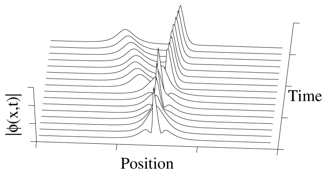
Figure 2: A typical example of the splitting of the second-order soliton under the action of a weak resonant modulation of the coefficient in front of the cubic nonlinearity, in the absence of the quintic term.

The simulations demonstrate that even a very weak resonant perturbation splits the second-order soliton, but the onset of the splitting requires time which increases with the decrease of the strength of the ac modulation, $b$. The smallest perturbation amplitude that we applied in the simulations was $b=5\times 10^{-5}$. This limitation was determined by the accumulation of numerical errors and available computational time; however, the results strongly suggest that there is no cutoff for the resonant splitting, as concerns the smallness of the perturbation amplitude.

For the quantitative analysis of the splitting, it is necessary to exactly define the splitting time, $T$. Figure 3 shows a generic example of the gradual decay of density oscillations of a second-order soliton in the course of its splitting. Following this picture, we define $T$ as the time elapsed from the start of the action of the NLM until the amplitude of the density oscillations drops to $10\%$ of its initial value in the 2-soliton. By that time, the second-order soliton turns into well-separated constituents. In fact, adopting another technical definition of the splitting time produces a little effect on the final results.

Figure 3: A detailed picture of the decay of density oscillations in the course of the splitting of a second-order soliton into its two fundamental constituents. Oscillations of the highest peak in the two-soliton waveform are shown during and after the splitting.

The chain of open squares in Fig. 4 shows the splitting time as a function of the perturbation strength, $b$ (in the case of $\epsilon=0$), revealing the divergence in the limit of $b\rightarrow 0$. We fit this dependence to a simple power-law expression,

$$T=a\cdot b^{p}+c$$ (8)

where $a,~{}c$ and $p<0$ are constant parameters and $b$ is taken in percents. As can be seen in the figure, the fitting formula captures the behavior of the numerical data well. For $\epsilon=0$, the fitting parameters are $p=-0.462\pm{0.022}$ and $a=(5.24\pm{0.59})\times 10^{3}$, $c=(1.44\pm{0.78})\times 10^{3}$.

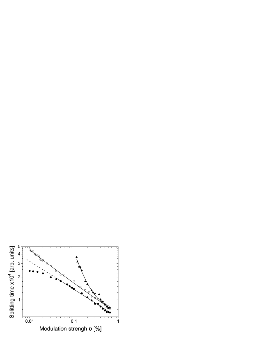
Figure 4: The splitting time of the 2-soliton, as produced by the simulations,versus the ac-drive’s amplitude, $b$. Open squares pertain to the case of the cubic nonlinearity only ($\epsilon=0$), black triangles are for $\epsilon=-9.1\times 10^{-4}$, and black circles are for $\epsilon=3.03\times 10^{-4}$. Solid lines show the fit provided by Eq. (8). For positive $\epsilon$, the fitting formula (shown by the dashed line in this region) does not describe the numerical data at smallest values of $b$, which indicates saturation for extremely weak perturbation strengths.

Further, black triangles and circles in Fig. 4 show the splitting time as a function of the NLM strength in the presence of the weak quintic nonlinearity of either sign, viz., for

$$\epsilon=-9.1\times 10^{-4}~{}~{}\mathrm{and}\mathsf{~{}~{}}\epsilon=3.03\times 10^{-4},$$ (9)

respectively. Even this very weak extra nonlinearity affects the splitting time dramatically: the additional quintic attraction (repulsion) delays (accelerates) the splitting, thus effectively stabilizing (destabilizing) the 2-soliton. In particular, the quintic self-focusing term with the amplitude as small as $\epsilon=-9.1\times 10^{-4}$ (black triangles in Fig. 4) is enough to increase the spitting time by a factor of $\sim 2.5$ when the ac-drive’s strength is $b=1\times 10^{-3}$, as compared to the case of $\epsilon=0$.

The fit parameters for the data pertaining to the extra quintic attraction or repulsion, with the values of $\epsilon$ as in Eq. (9), are, respectively,

$$p=-1.93\pm{0.16},~{}~{}a=(4.2\pm{1.5})\times 10^{2},~{}~{}c=(7.25\pm{0.53})\times 10^{3},$$ (10)

$$p=-0.372\pm{0.007,~{}}a=(5.84\pm{0.09})\times 10^{3},~{}c=0.$$ (11)

It is worth noting the differences in parameter $c$ for both cases. For $\epsilon<0$, positive $c$ in the fitting set (10) means that, even for a strong perturbation, a final waiting time is required to observe the splitting of the 2-soliton, which is another manifestation of its stabilization by the quintic self-focusing term. On the contrary, for $\epsilon>0$, the best fit actually required to choose $c<0$–in the parameter region where formula (8) with $c<0$ produces $T>0$. Setting $c=0$ in the fitting set (11) means that the simulations demonstrate that the 2-soliton starts splitting instantaneously under the action of the strong resonant perturbation.

Actually, for large perturbation amplitudes ($b>0.02$), the splitting produces fundamental solitons with the amplitude ratio different from $1:3$, which may be explained by effects induced by the relatively strong perturbation on the constituents of the 2-soliton in the course of the splitting. In the case of the self-defocusing quintic nonlinearity, $\epsilon>0$, the splitting time shows saturation for extremely weak perturbations (see black circles in Fig. 4), i.e., the splitting time ceases to grow with further weakening of the perturbation. A plausible explanation to this feature, which demonstrates the fragility of the second-order soliton in this situation, is the fact that splitting is spontaneously initiated by the numerical noise. We also note that the quintic nonlinearity slightly changes the frequency of the shape oscillations of the 2-soliton, see Fig. 1. The modulation frequency was modified, accordingly, in the simulations, to maintain the resonance condition for all cases included in Fig. 4.

Figure 5 summarizes absolute values of exponent $|p|$, i.e., the best-fit parameter in Eq. (8), as a function of strength $\epsilon$ of the quintic nonlinearity. The error bars in the figure represent errors of the fit to the power-law approximation defined as per Eq. (8). For $\epsilon<0$, $|p|$ rapidly increases with $-\epsilon$, indicating that the second-order soliton develops strong resistance against the resonant splitting, with the enhancement of the quintic self-focusing. On the other hand, $|p|$ drops for $\epsilon>0$, showing the destabilization of the second-order soliton under the action of the quintic self-defocusing.

Figure 5: The power-law fit parameter, $|p|$, from Eq. (8), as a function of the strength of the quintic nonlinearity, $\epsilon$. The error bars represent the error of the fit to formula (8).

II.3 The near-resonance response

In Ref. Sakaguchi04 it was shown that the splitting of the 2-soliton (in the case of $\epsilon=0$) could also be caused by the temporal modulation of the coefficient in front of the cubic term with the frequency slightly different from resonant value (4). Here, we aim to confirm this behavior for case of the cubic NLSE and extend the analysis to the CQ model, with $\epsilon\neq 0$ (in the latter case, the resonant frequency should be first slightly adjusted, as mentioned above). For this purpose, we have performed the simulations by varying modulation strength $b$ at fixed values of the driving frequency and fitting the so observed splitting time ($T$) to the power-law function, defined as per Eq. (8).

Figure 6 displays the absolute value of the fitting power, $|p|$, versus the modulation frequency, for four different values of the quintic-nonlinearity coefficient, $\epsilon=-1.6\times 10^{-3}$ (open rhombuses), $\epsilon=-7.6\times 10^{-4}$ (black triangles), $\epsilon=0$ (open squares), and $\epsilon=7.6\times 10^{-4}$ (black circles). As before, the error bars in the figure represent errors of the fit. Two noteworthy features are clearly seen in the figure. First, small and large values of $|p|$ are obtained for the repulsive and attractive quintic nonlinearity, respectively, in accordance with what was reported above for the case of the exact resonance. Second, in most cases the presence of the quintic term of either sign gives rise to broadening of the resonant response, in comparison with the case of the pure cubic nonlinearity (represented by open squares in Fig. 6; the broadening is weak in the case of the weakest quintic self-focusing, which corresponds to $\epsilon=-7.6\times 10^{-4}$, which is represented by the chain of black triangles). In the case of the repulsive quintic nonlinearity, $\epsilon>0$, the dependence shown by the circles in Fig. 6 is nearly flat, i.e., the second-order soliton readily splits even at a relatively large detuning from the resonance. On the contrary, the stabilization of the 2-soliton by the self-focusing quintic nonlinearity is seen to be robust also under the off-resonance conditions.

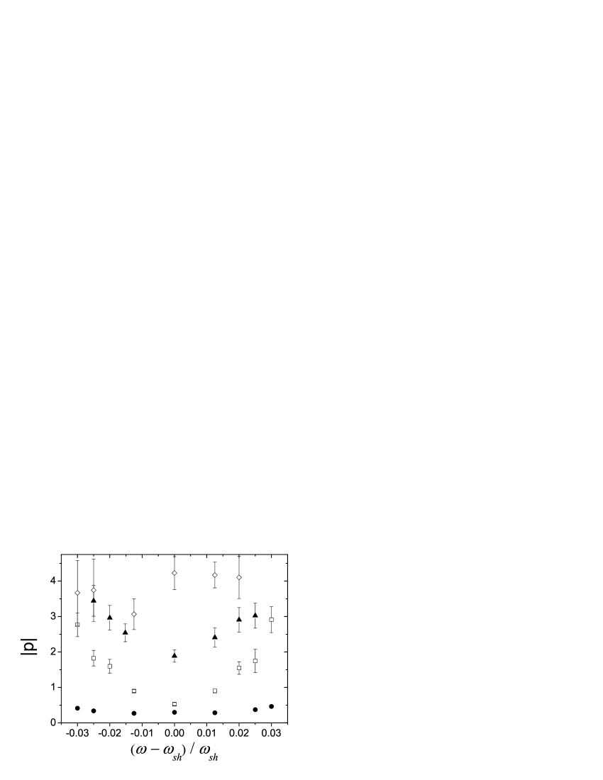
Figure 6: The power-law fit parameter, $|p|$, as a function of the modulation frequency. Open squares, black triangles, open rhombes, and black circles are, respectively, for the pure cubic nonlinearity ($\epsilon=0$), $\epsilon=-7.6\times 10^{-4}$, $\epsilon=-1.6\times 10^{-3}$ (the self-focusing quintic term), and $\epsilon=7.6\times 10^{-4}$ (the self-defocusing one). The error bars represent errors of the fit to the power-law expression defined as per Eq. (8).

III Analytical estimates

A qualitative explanation to some numerical findings reported above can be provided by an analytical consideration of the model based on Eq. (1). First, it is possible to explain the underlying effect of the resonant splitting of the 2-soliton. Indeed, as mentioned above, the binding energy of the higher-order solitons is exactly zero in the integrable NLSE, therefore the splitting may be explained by the fact that the resonant temporal modulation pumps energy into the bound 2-soliton state, causing its splitting into constituents, which carry away the excess energy, in the form of their kinetic energies. In the presence of the small modulation term in the cubic coefficient given by Eq. (7), whose frequency is set to coincide with the resonant value (4), the exact evolution equation for energy $E_{0}$ of the unperturbed NLSE, i.e., Eq. (2) with $g=1$ and $\epsilon=0$, can be derived in the following form:

$$\frac{dE_{0}}{dt}=b\sin\left(4A^{2}t\right)\int_{-\infty}^{+\infty}\mathrm{Im}\left\{\left(\frac{\partial\phi}{\partial x}\right)^{2}\left(\phi^{\ast}\right)^{2}\right\}dx.$$ (12)

In the lowest approximation, one can substitute the unperturbed 2-soliton solution, as given by Eq. (5), into the right-hand side of Eq. (12). Under the condition that the shape oscillations of the 2-soliton are synchronized with the temporal modulation in Eq. (7) (analysis of of numerical results confirms this conjecture, in the case of the slowly developing splitting), the time averaging of Eq. (12) yields an effective energy-pump rate,

$$\left\langle\frac{dE_{0}}{dt}\right\rangle=\frac{128}{\pi}C_{b}A^{5}b\approx~{}23.2~{}A^{5}b,$$ (13)

where the constant is given by the following integral expression,

$$C_{b} = \left|\int_{0}^{2\pi}d\tau\sin\tau\int_{-\infty}^{+\infty}d\xi~{}\mathrm{Im}\left\{\left[\frac{\cosh\left(3\xi\right)+3e^{-i\tau}\cosh\xi}{\cosh\left(4\xi\right)+4\cosh\left(2\xi\right)+3\cos\tau}\right]^{2}\right.\right.$$ (14)

$$\times\left.\left.\left[\frac{\partial}{\partial\xi}\frac{\cosh\left(3\xi\right)+3e^{i\tau}\cosh\xi}{\cosh\left(4\xi\right)+4\cosh\left(2\xi\right)+3\cos\tau}\right]^{2}\right\}\right|~{}\approx 0.57.$$

This explanation of the gradual onset of the splitting of the 2-soliton through the pumping of the energy into it by the resonant NLM was not considered in Ref. Sakaguchi04 , which was dealing with the (near-)resonant splitting in the cubic NLSE (with $\epsilon=0$).

The stabilization/destabilization of the 2-soliton by the self-focusing/defocusing quintic nonlinearity may also be explained by means of the consideration of the energy. In expression (2), the term corresponding to the quintic nonlinearity in Eq. (1) yields the following expression for the additional energy, obtained by the substitution of the unperturbed 2-soliton solution (5) and averaging over the period of its shape oscillations:

$$\left\langle\Delta E_{\mathrm{2-soliton}}\right\rangle=\left(2^{11}C_{\epsilon}/3\pi\right)A^{5}\epsilon\approx~{}39.5~{}A^{5}\epsilon,$$ (15)

with constant

$$C_{\epsilon}=\int_{0}^{2\pi}d\tau\int_{-\infty}^{+\infty}d\xi~{}\frac{\left\{\left[\cosh\left(3\xi\right)+3\left(\cos\tau\right)\cosh\xi\right]^{2}+\left(\sin^{2}\tau\right)\cosh^{2}\xi\right\}^{3}}{\left[\cosh\left(4\xi\right)+4\cosh\left(2\xi\right)+3\cos\tau\right]^{6}}~{}\approx 0.18.$$

Finally, the binding energy of the 2-soliton induced by the quintic term can be defined as the difference between the respective extra energies of the pair of free fundamental solitons, with amplitudes $3A$ and $A$, into which the 2-soliton splits, $\Delta E_{3A+A}=\left(3^{5}+1\right)(16/45)\epsilon A^{5}\approx 86.8~{}\epsilon A^{5}$, and energy (15) of the unsplit bound state:

$$\Delta E=\Delta E_{3A+A}-\Delta E_{\mathrm{2-soliton}}\approx 47.3~{}\epsilon A^{5}.$$ (16)

The negativeness and positiveness of expression (16) for $\epsilon<0$ and $\epsilon>0$, respectively, explains the stabilization/destabilization of the 2-soliton by the self-focusing/defocusing quintic nonlinearity.

According to Eq. (13), under the action of the resonant NLM the energy of the resonantly driven 2-soliton grows, on the average, linearly in time:

$$E_{0}(t)\approx E_{0}(0)+~{}23.2~{}A^{5}bt,$$ (17)

where the initial value, $E_{0}(0)$, is energy (6) of the unperturbed 2-soliton. If all the energy pumped by the NLM drive would be accumulated in the form of the “splitting potential”, then, in the case of $\epsilon<0$, the onset of the splitting might be expected at the moment of time when this stored “potential” becomes equal to the binding energy, which would give the splitting time as $T=\Delta E/\left\langle dE_{0}/dt\right\rangle$. In its literal form, this result implies $p=-1$ in Eq. (8). The deviation of actual values of $|p|$ from $1,$ as seen in Fig. 5, is explained by the fact that, within the framework of the present analysis, it is not known how the pumped energy is divided between the actual accumulation of the splitting potential and absorption into a change of the unperturbed 2-soliton’s energy – see Eq. (6) – due to a possible small variation of $A$. While an exact prediction of $|p|$ as a function of $\epsilon$ seems to be too difficult for the fully analytical treatment, the fact that, according to Fig. 5, $|p|$ is essentially larger than $1$ at $-\epsilon>10^{-3}$ suggests that, in this range of values of $\epsilon$, nearly all the pumped energy is absorbed into the increase of the 2-soliton’s energy. Combining Eqs. (6) and (17), one can conclude that, as long as the resulting deviation of amplitude $A$ from its initial value, $A_{0}$, remains small, the amplitude varies in time as $A(t)\approx A_{0}-\allowbreak 0.8A_{0}^{3}b\cdot t$. This variation leads to a detuning of the resonant driving, according to Eq. (4), but, on the other hand, Fig. 6 demonstrates that the detuning does not produce an essential effect for $-\epsilon>10^{-3}$.

IV Conclusions

In this work we have considered the influence of the weak quintic nonlinearity on the stability and splitting of second-order solitons (alias 2-solitons) in the NLSE-based model, under the action of the weak resonant NLM (nonlinearity management), i.e., periodic time modulation of the coefficient in front of the cubic term, with the frequency equal or close to the frequency of the free shape oscillations of the 2-soliton. The model applies to the propagation of light in CQ optical media, taking into regard the periodic action of the linear loss and compensating gain. The same model finds a natural application to BEC, where the self-focusing quintic term accounts for the effect of the residual three-dimensionality in the effective one-dimensional approximation, while the NLM may be induced by the Feshbach resonance controlled by an ac magnetic field. By means of direct simulations and an approximate analytical considerations, we have demonstrated that the additional weak self-focusing quintic nonlinearity stabilizes the 2-soliton, while the self-defocusing nonlinearity of the same type makes it fragile and accelerates its splitting. We have confirmed the resonant character of the splitting of the 2-soliton under the action of the NLM, and proposed an explanation to this effect, based on the consideration of the rate at which the energy is pumped into the bound state by the resonantly tuned ac drive. We have also studied the resonant NLM-induced splitting of the 2-soliton in the presence of the weak quintic nonlinearity. Depending on its sign, the self-defocusing/focusing higher-order nonlinearity gives rise to conspicuous broadening/sharpening of this resonant response. The results of the numerical and analytical considerations reported in this paper for 2-solitons can be readily extended to higher-order solitons.

References

- (1) B. A. Malomed, Soliton Management in Periodic Systems (Springer: New York, 2006).
- (2) S. Novikov, S. V. Manakov, L. P. Pitaevskii, and V. E. Zakharov, Theory of Solitons (Consults Bureau, New York, 1984).
- (3) G. P. Agrawal, Nonlinear Fiber Optics (Academic Press: San Diego, 2001); A. Hasegawa and Y. Kodama, Solitons in Optical Communication (Oxford University Press: New York, 2004).
- (4) B. A. Malomed, D. F. Parker, and N. F. Smyth, Phys. Rev. E 48, 1418 (1993).
- (5) R. G. Bauer, L. A. Melnikov, Opt. Commun. 115, 190 (1995).
- (6) A. A. Sysoliatin, A. K. Senatorov, A. I. Konyukhov, L. A. Melnikov, and V. A. Stasyuk, Opt. Express 15, 16302 (2008).
- (7) A. Hasegawa and Y. Kodama, Phys. Rev. Lett. 66, 161 (1991).
- (8) C. Paré, A. Villeneuve, P.-A. Belangé, and N. J. Doran, Opt. Lett. 21, 459 (1996); C. Paré, A. Villeneuve, and S. LaRochelle, Opt. Commun. 160, 130 (1999).
- (9) R. Driben, B. A. Malomed, M. Gutin, and U. Mahlab, Opt. Commun. 218, 93 (2003).
- (10) R. Driben, B. A. Malomed, and U. Mahlab, Opt. Commun. 232, 129 (2004).
- (11) L. P. Pitaevskii and S. Stringari, Bose–Einstein Condensation (Clarendon Press: Oxford, 2003; ISBN 0-198-50719-4).
- (12) P. G. Kevrekidis, G. Theocharis, D. J. Frantzeskakis and B. A. Malomed, Phys. Rev. Lett. 90, 230401 (2003).
- (13) R. Grimshaw, J. He, and B. A. Malomed, Phys. Scripta 53, 385 (1996).
- (14) H. Sakaguchi and B. A. Malomed, Phys. Rev. E 70, 066613 (2004).
- (15) G. S. Agarwal and S. Dutta Gupta, Phys. Rev. A 38, 5678 (1988).
- (16) E. L. Falcão-Filho, C. B. de Araújo, and J. J. Rodrigues, Jr., J. Opt. Soc. Am. B 24, 2948 (2007).
- (17) R. A. Ganeev, M. Baba, M. Morita, A. I. Ryasnyansky, M. Suzuki, M. Turu, and H. Kuroda, J. Opt. A: Pure Appl. Opt. 6, 282 (2004).
- (18) B. Gu, Y. Wang, W. Ji, and J. Wang, Appl. Phys. Lett. 95, 041114 (2009).
- (19) K. Dolgaleva, R. W. Boyd, J. E. Sipe, Phys. Rev. A 76, 063806 (2007).
- (20) F. Smektala, C. Quemard, V. Couderc, A. Barthéĺémy, J. Non-Cryst. Solids 274, 232 (2000); K. Ogusu, J. Yamasaki, S. Maeda, M. Kitao, and M. Minakata, Opt. Lett. 29, 265 (2004); C. Zhan, D. Zhang, D. Zhu, D. Wang, Y. Li, D. Li, Z. Lu, L. Zhao, and Y. Nie, J. Opt. Soc. Am. B 19, 369 (2002); G. Boudebs, S. Cherukulappurath, H. Leblond, J. Troles, F. Smektala, and F. Sanchez, Opt. Commun. 219, 427 (2003).
- (21) A. E. Muryshev, G. V. Shlyapnikov, W. Ertmer, K. Sengstock, and M. Lewenstein, Phys. Rev. Lett. 89, 110401 (2002); S. Sinha, A. Y. Cherny, D. Kovrizhin, and J. Brand, ibid. 96, 030406 (2006).
- (22) L. Salasnich, Laser Phys. 12, 198 (2002); L. Salasnich, A. Parola, and L. Reatto, Phys. Rev. A 65, 043614 (2002).
- (23) L. Khaykovich and B. A. Malomed, Phys. Rev. A 74, 023607 (2006).
- (24) Yu. Kagan, A. E. Muryshev, and G. V. Shlyapnikov, Phys. Rev. Lett. 81, 933 (1998); F. Kh. Abdullaev, A. Gammal, L. Tomio, and T. Frederico, Phys. Rev. A 63, 043604 (2001).
- (25) J. Satsuma and N. Yajima, Progr. Theor. Phys. Suppl. 55, 284 (1974).
- (26) Kh. I. Pushkarov, D. I. Pushkarov, and I. V. Tomov, Opt. Quant. Electr. 11, 471 (1979); S. Cowan, R. H. Enns, S. S. Rangnekar, and S. S. Sanghera Can. J. Phys. 64, 311 (1986).