Broadband adiabatic conversion of light polarization

Abstract

A broadband technique for robust adiabatic rotation and conversion of light polarization is proposed. It uses the analogy between the equation describing the polarization state of light propagating through an optically anisotropic medium and the Schrödinger equation describing coherent laser excitation of a three-state atom. The proposed technique is analogous to the stimulated Raman adiabatic passage (STIRAP) technique in quantum optics; it is applicable to a wide range of frequencies and it is robust to variations in the propagation length and the rotary power.

I Introduction

A simple way to describe the polarization state of light, which has been known for many years in optics, is by the Stokes vector, which is depicted as a point on the so-called Poincaré sphere Born ; Kubo80 ; Kubo81 ; Kubo83 ; Rothmayer09 . The Stokes vector, for instance, is a particularly convenient tool to describe the change of the polarization state of light transmitted through anisotropic optical media Kubo80 ; Kubo81 ; Kubo83 .

The equation of motion for the Stokes vector in a medium with zero polarization dependent loss (PDL) has a torque form Sala ; Gregori ; Tratnik . This fact has been used recently to draw analogies between the motion of the Stokes vector and a spin-$\frac{1}{2}$ particle in nuclear magnetic resonance and an optically driven two-state atom in quantum optics, both described by the Schrödinger equation Kuratsuji98 ; Zapasskii ; Seto05 ; Kuratsuji07 .

Here we propose a technique for controlled robust conversion of the polarization of light transmitted through optically anisotropic media with no PDL. The technique is analogous to stimulated Raman adiabatic passage (STIRAP) in quantum optics Gau90 ; Ber98 ; Vit01b and hence enjoys the same advantages as STIRAP in terms of efficiency and robustness.

For any traditional polarization devices the rotary power (the phase delay between the fast and slow eigenpolarizations) scales in proportion to the frequency of the light and thus such devices are frequency dependent: a half-wave plate is working for exactly one single frequency. On the contrary, the adiabatic polarization conversion proposed here is frequency independent: any input polarization will be transformed to the same output polarization state regardless of the wavelength. It acts intrinsically as a broadband device limited only by the absorptive characteristics of the device instead of its birefringence bandwidth. Moreover, the proposed technique is robust against variations in the length of the device, in the same fashion as quantum-optical STIRAP is robust against variations in the pulse duration.

II Stokes polarization vector

We first consider a plane electromagnetic wave traveling through a dielectric medium in the $z$ direction. The medium is anisotropic and with no PDL, therefore the polarization evolution is given with the following torque equation for the Stokes vector Kubo80 ; Kubo81 ; Kubo83 ; Sala ; Gregori ; Tratnik ; Kuratsuji98 ; Seto05 ; Kuratsuji07 :

$$\frac{\,\text{d}}{\,\text{d}z}\mathbf{S}(z)=\mathbf{\Omega}(z)\times\mathbf{S}(z),$$ (1)

where $z$ is the distance along the propagation direction, and $\mathbf{S}(z)=[S_{1}(z),S_{2}(z),S_{3}(z)]$ is the Stokes polarization vector shown in Fig. 1. Every Stokes polarization vector corresponds to a point on the Poincaré sphere and vice versa. The right circular polarization is represented by the north pole, the left circular polarization by the south pole, the linear polarizations by points in the equatorial plane, and the elliptical polarization by the points between the poles and the equatorial plane. $\mathbf{\Omega}(z)=[\Omega_{1}(z),\Omega_{2}(z),\Omega_{3}(z)]$ is the birefringence vector of the medium: the direction of $\mathbf{\Omega}(z)$ is given by the slow eigenpolarization and its length $|\mathbf{\Omega}(z)|$ corresponds to the rotary power.

III Schrödinger equation for a three-state quantum system

When one of the components of the vector $\mathbf{\Omega}(z)$ is zero, then Eq. (1) is mathematically equivalent to the Schrödinger equation for a coherently driven three-state quantum $\Lambda$ system on exact resonances with the carrier frequencies of the external fields. This is readily seen by examining the time-dependent Schrödinger equation, which in the rotating-wave approximation (RWA) reads

$$\text{i}\hbar\frac{\text{d}}{\text{d}t}\mathbf{c}(t)=\mathbf{H}(t)\mathbf{c}(t).$$ (2)

Here $\mathbf{c}(t)$ is a column vector of the probability amplitudes $c_{n}(t)$ ($n=1,2,3$) of the three states $\psi_{1}$, $\psi_{2}$ and $\psi_{3}$, and $\mathbf{H}(t)$ is a $3\times 3$ Hamiltonian matrix Gau90 ; Ber98 ; Vit01b ,

$$\mathbf{H}(t)=\frac{\hbar}{2}\left[\begin{array}[]{ccc}0&\Omega_{1}(t)&0\\ \Omega_{1}(t)&0&\Omega_{2}(t)\\ 0&\Omega_{2}(t)&0\end{array}\right].$$ (3)

We have here assumed both two-photon and single-photon resonances. The two slowly varying Rabi frequencies $\Omega_{1}(t)$ and $\Omega_{2}(t)$ parameterize the strengths of each of the two fields; they are proportional to the dipole transition moments $\mathbf{d}_{ij}$ and to the electric-field amplitudes $\mathbf{E}_{k}(t)$: $\Omega_{1}(t)=-\mathbf{d}_{12}\mathbf{\cdot E}_{1}(t)$ and $\Omega_{2}(t)=-\mathbf{d}_{23}\mathbf{\cdot E}_{2}(t)$; hence each of them varies as the square root of the corresponding intensity.

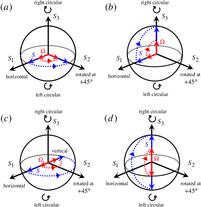
Figure 1: (Color online) Poincaré sphere representation of polarization states. The Stokes polarization vector $\mathbf{S}(z)$ follows adiabatically the birefringence vector $\mathbf{\Omega}(z)$. (a) Linear polarization is rotated by $45^{\circ}$ (corresponding to $90^{\circ}$ rotation of the Stokes vector); (b) linear polarization is transferred into right circular polarization; (c) horizontal linear polarization is transferred into vertical linear polarization; (d) left circular polarization is transferred into right circular polarization.

The quantum evolution associated with the $\Lambda$ system is easily understood with the use of adiabatic states, i.e. the three instantaneous eigenstates $\varphi_{k}(t)$ of the RWA Hamiltonian (3). The adiabatic state $\varphi_{0}(t)$ corresponding to a zero eigenvalue is particularly noteworthy, because it has no component of state $\psi_{2}$,

$$\varphi_{0}(t)=\frac{\Omega_{2}(t)}{\sqrt{\Omega_{1}^{2}(t)+\Omega_{2}^{2}(t)}}\psi_{1}-\frac{\Omega_{1}(t)}{\sqrt{\Omega_{1}^{2}(t)+\Omega_{2}^{2}(t)}}\psi_{3}.$$ (4)

This state therefore does not lead to fluorescence and is known as a dark state Gau90 ; Ber98 ; Vit01b . If the motion is adiabatic Gau90 ; Ber98 ; Vit01b , and if the state vector $\Psi(t)$ is initially aligned with the adiabatic state $\varphi_{0}(t)$, then the state vector remains aligned with $\varphi_{0}(t)$ throughout the evolution. This occurs if the pulses are ordered counterintuitively, $\Omega_{2}(t)$ before $\Omega_{1}(t)$: then the composition of the dark state $\varphi(t)$ will progress from initial alignment with $\psi_{1}$ to final alignment with $\psi_{3}$. Hence in the adiabatic regime the complete population will be transferred adiabatically from state $\psi_{1}$ to state $\psi_{3}$. This important feature of complete transfer under full control has made STIRAP a widespread preparation technique for experiments relying on precise state control Ber98 ; Vit01b . The formalism can be applied to other systems, including classical ones Suchowski08 ; Suchowski09 ; Rangelov09 , by making use of the similarity of the respective equations to Eqs. (2) and (3).

IV Adiabatic conversion of light polarization

Returning to light polarization, two special cases are particularly interesting.

Case A: $\Omega_{3}(z)=0$. With the redefinition of variables $S_{1}(t)=-ic_{3}(t),\quad S_{2}(t)=ic_{1}(t),\quad S_{3}(t)=-c_{2}(t)$, the Schrödinger equation (2) turns into the form (1), if we map the time dependance into the coordinate dependance. By using this analogy we can write down a superposition $\sigma(z)$ of the polarization components $S_{1}(z)$ and $S_{2}(z)$ of the Stokes vector, which corresponds to the dark state $\varphi_{0}(t)$, Eq. (4):

$$\sigma(z)=\frac{\Omega_{1}(z)S_{1}(z)+\Omega_{2}(z)S_{2}(z)}{|\mathbf{\Omega}(z)|}.$$ (5)

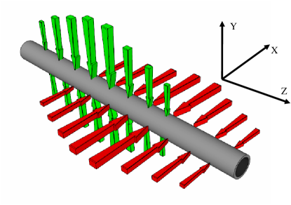
Figure 2: (Color online) Fiber optics setup with overlapping horizontal and vertical linear birefringent sections induced by z dependent stress (Case A). The magnitude of horizontal and vertical stress is represented by initially increasing then decreasing, in length, red and green arrows.

When $\Omega_{1}(z)$ precedes $\Omega_{2}(z)$ the polarization superposition (5) has the following asymptotic values

$$S_{1}(z_{i})\overset{z_{i}\leftarrow z}{\longleftarrow}\sigma(z)\overset{z\rightarrow z_{f}}{\longrightarrow}S_{2}(z_{f}).$$ (6)

Thus if initially the light is linearly polarized in horizontal direction, $\mathbf{S}(z_{i})=(1,0,0)$, we end up with a linearly polarized light rotated by $45^{\circ}$, $\mathbf{S}(z_{f})=(0,1,0)$ (see Fig. 1 (a)). The process is reversible; hence if we start with a linear polarization rotated by $45^{\circ}$ and apply a reverse field order ($\Omega_{2}(z)$ preceding $\Omega_{1}(z)$) this will lead to reversal of the direction of motion and we will end up with a linear polarization in a horizontal direction.

Following quantum-optical STIRAP, we can write down the condition for adiabatic evolution as Ber98 ; Vit01b

$$\int_{0}^{L}|\mathbf{\Omega}(z)|\,dz\gg 1.$$ (7)

For example, for adiabatic evolution it suffices to have $\int_{0}^{L}|\mathbf{\Omega}(z)|\,dz\gtrsim 6\pi$. Here $L$ is the thickness of the medium and the length of the birefringence vector is given by $|\mathbf{\Omega}(z)|=2\pi\Delta n/\lambda$, where $\lambda$ is the wavelength of the light, $\Delta n$ is the difference between the refractive indices for ordinary and extraordinary rays. Then the adiabatic condition reads

$$L\Delta n\gtrsim 3\lambda.$$ (8)

The last condition shows that the process is robust against variation in the parameters, for example, the wavelength $\lambda$ and the propagation length $L$. This condition is readily fulfilled, by orders of magnitude, in many birefringent materials.

Case B: $\Omega_{2}(z)=0$. Following a similar argumentation as for Case A and interchanging the Stokes vector components $S_{1}(z)$ and $S_{3}(z)$ we can write down a “dark” superposition $\sigma(z)$ of the polarization components $S_{1}(z)$ and $S_{3}(z)$ of the Stokes vector,

$$\sigma(z)=\frac{\Omega_{1}(z)S_{1}(z)+\Omega_{3}(z)S_{3}(z)}{\left|\mathbf{\Omega}(z)\right|}.$$ (9)

If initially the light is linearly polarized, $\mathbf{S}(z_{i})=(1,0,0)$, then by arranging $\Omega_{1}(z)$ to precede $\Omega_{3}(z)$, we end up with a right circular polarization, $\mathbf{S}(z_{f})=(0,0,1)$, as depicted by the north pole on the Poincaré sphere in Fig. 1 (b), because the polarization superposition (9) has the asymptotic values

$$S_{1}(z_{i})\overset{z_{i}\leftarrow z}{\longleftarrow}\sigma(z)\overset{z\rightarrow z_{f}}{\longrightarrow}S_{3}(z_{f}).$$ (10)

The process is again reversible: starting with a right circular polarization, and applying $\Omega_{3}(z)$ before $\Omega_{1}(z)$ we end up with a linear polarization.

We note that a numerical prediction of broadband conversion from circular polarized light into linearly polarized light for the wavelength range 434 nm to 760.8 nm for crystalline quartz was made by Darsht et al. Darsht . Here this effect emerges as a special case of our general adiabatic frame of STIRAP analogy.

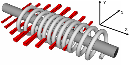
Figure 3: (Color online) Similar to Fig. 2 except that the stress induced linear birefringence has been replaced by an circular birefringent section generated through the Faraday effect and a magnetic field along z direction (Case B). The increasing and decreasing number of turns in the spool indicate changes in magnetic field.

The adiabatic polarization conversion could be demonstrated with a single-mode fiber, which exhibits both stress-induced linear birefringence and circular birefringence (either by the Faraday effect or by a torsion of the fiber) Born . Possible implementations are depicted in Figs. 2 (for Case A) and 3 (for Case B).

The technique proposed here is not limited to linear-linear or circular-linear conversions, but it is also applicable for arbitrary transformations of light polarization. For example the conversion between right circular and left circular polarization is analogous to adiabatic passage via a level crossing Vit01b . To this end, we first start up with $\Omega_{3}(z)$, then we activate $\Omega_{1}(z)$, then let $\Omega_{3}(z)$ change sign while $\Omega_{1}(z)$ is having its maximal value, and then gradually make $\Omega_{3}(z)$ to fade away.

We can also change the polarization from linear to elliptical if we first begin with $\Omega_{1}(z)$, then we activate $\Omega_{3}(z)$, and then let $\Omega_{1}(z)$ and $\Omega_{3}(z)$ simultaneously fade away [cf. Eq. (9)]; this sequence is known in quantum optics as fractional STIRAP Half-STIRAP .

V Exact solution

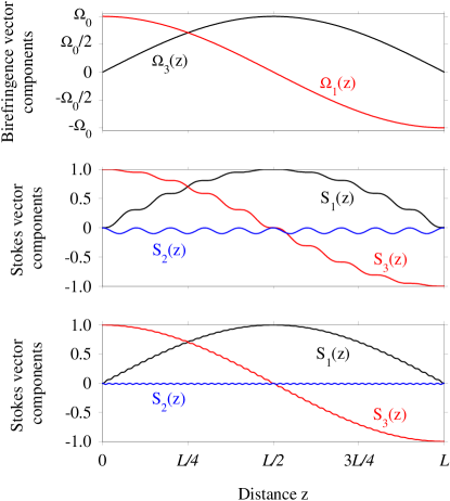
Figure 4: (Color online) Top frame: birefringence vector components as a function of the propagation length when the components are given as in Eq. (11). Middle frame: the evolution of the Stokes polarization vector components for $\Omega_{0}=20/L$, adiabatic evolution start to work. Bottom frame: the evolution of the Stokes polarization vector components for $\Omega_{0}=100/L$ with better adiabatic evolution, smaller ripples on the curves, compare with the middle frame.

As an example of polarization conversion we present here an exact analytic solution to the Stokes polarization equation (1) for the slowly varying birefringence components given by trigonometric functions:

$$\Omega_{1}(z) =\Omega_{0}\sin(z\pi/L),$$ (11a)

$$\Omega_{3}(z) =\Omega_{0}\cos(z\pi/L).$$ (11b)

We assume that initially the Stokes vector is $\mathbf{S}(z=0)=(0,0,1)$, i.e. the polarization is right circular. Then the solution for the Stokes vector components as a function of $z$ reads

$$S_{1}(z) =\frac{\Omega_{0}^{2}L^{2}+\cos\big{(}\pi z\sqrt{\Lambda^{2}+\Omega_{0}^{2}}\big{)}}{1+\Omega_{0}^{2}L^{2}}\sin\left(\frac{\pi z}{L}\right)$$

$$-\frac{\sin\big{(}\pi z\sqrt{\Lambda^{2}+\Omega_{0}^{2}}\big{)}}{\sqrt{1+\Omega_{0}^{2}L^{2}}}\cos\left(\frac{\pi z}{L}\right),$$ (12a)

$$S_{2}(z) =\frac{2\Omega_{0}L}{1+\Omega_{0}^{2}L^{2}}\sin^{2}\left(\frac{\pi z}{2}\sqrt{\Lambda^{2}+\Omega_{0}^{2}}\right),$$ (12b)

$$S_{3}(z) =\frac{\Omega_{0}^{2}L^{2}+\cos\big{(}\pi z\sqrt{\Lambda^{2}+\Omega_{0}^{2}}\big{)}}{1+\Omega_{0}^{2}L^{2}}\cos\left(\frac{\pi z}{L}\right)$$

$$+\frac{\sin\big{(}\pi z\sqrt{\Lambda^{2}+\Omega_{0}^{2}}\big{)}}{\sqrt{1+\Omega_{0}^{2}L^{2}}}\sin\left(\frac{\pi z}{L}\right),$$ (12c)

where $\Lambda=1/L$. The adiabatic evolution takes place when $\Omega_{0}L\gg 1$;

For $z=L/2$ (quarter period) we have

$$S_{1}(L/2) =\frac{\Omega_{0}^{2}L^{2}+\cos\big{(}\frac{\pi}{2}\sqrt{1+\Omega_{0}^{2}L^{2}}\big{)}}{1+\Omega_{0}^{2}L^{2}}\overset{\Omega_{0}L\gg 1}{\longrightarrow}1,$$ (13a)

$$S_{2}(L/2) =\frac{2\Omega_{0}L}{1+\Omega_{0}^{2}L^{2}}\sin^{2}\left(\frac{\pi}{4}\sqrt{1+\Omega_{0}^{2}L^{2}}\right)\overset{\Omega_{0}L\gg 1}{\longrightarrow}0,$$ (13b)

$$S_{3}(L/2) =\frac{\sin\big{(}\frac{\pi}{2}\sqrt{1+\Omega_{0}^{2}L^{2}}\big{)}}{\sqrt{1+\Omega_{0}^{2}L^{2}}}\overset{\Omega_{0}L\gg 1}{\longrightarrow}0.$$ (13c)

This case exemplifies the conversion between circular and linear polarization via STIRAP-like adiabatic process, as illustrated in Fig. 4 (at the point $z=L/2$).

For $z=L$ (half period) we have

$$S_{1}(L) =\frac{\sin\big{(}\pi z\sqrt{\Lambda^{2}+\Omega_{0}^{2}}\big{)}}{\sqrt{1+\Omega_{0}^{2}L^{2}}}\overset{\Omega_{0}L\gg 1}{\longrightarrow}0,$$ (14a)

$$S_{2}(L) =\frac{2\Omega_{0}L}{1+\Omega_{0}^{2}L^{2}}\sin^{2}\left(\frac{\pi z}{2}\sqrt{\Lambda^{2}+\Omega_{0}^{2}}\right)\overset{\Omega_{0}L\gg 1}{\longrightarrow}0,$$ (14b)

$$S_{3}(L) =-\frac{\Omega_{0}^{2}L^{2}+\cos\big{(}\pi z\sqrt{\Lambda^{2}+\Omega_{0}^{2}}\big{)}}{1+\Omega_{0}^{2}L^{2}}\overset{\Omega_{0}L\gg 1}{\longrightarrow}-1.$$ (14c)

This case exemplifies the conversion between right circular and left circular polarization via level crossing adiabatic process, which is illustrated in Fig. 4 (at the point $z=L$).

VI Conclusion

In conclusion, we have shown that the powerful technique of STIRAP, which is well-known in quantum optics, has an analogue in the evolution of light polarization described by the equation for the Stokes vector. The factor that enables this analogy is the equivalence of the Schrödinger equation for a resonant three-state $\Lambda$ system, to the torque equation for the Stokes vector. The proposed technique transforms polarization with the same efficiency and robustness as STIRAP, therefore a polarization device based on this scheme is frequency independent and it is robust against variations of the propagation length, in contrast to the other well-known methods for conversion of light polarization.

This work has been supported by the European Commission projects EMALI and FASTQUAST, the Bulgarian NSF grants D002-90/08, DMU02-19/09 and Sofia University Grant 074/2010. We are grateful to Klaas Bergmann for useful discussions.

References

- (1) M. Born and E. Wolf, Principles of Optics (Pergamon, Oxford, 1975).
- (2) H. Kubo and R. Nagata, Opt. Commun. 34, 306 (1980).
- (3) H. Kubo and R. Nagata, J. Opt. Soc. Am. 71, 327 (1981).
- (4) H. Kubo and R. Nagata, “Vector representation of behavior of polarized light in a weakly inhomogeneous medium with birefringence and dichroism”, J. Opt. Soc. Am. 73, 1719 (1983).
- (5) M. Rothmayer, D. Tierney, E. Frins, W. Dultz, and H. Schmitzer, Phys. Rev. A 80, 043801 (2009).
- (6) K. L. Sala, Phys. Rev. A 29, 1944 (1984).
- (7) G. Gregori and S. Wabnitz, Phys. Rev. Lett. 56, 600 (1986).
- (8) M. V. Tratnik and J. E. Sipe, Phys. Rev. A 35, 2975 (1987).
- (9) H. Kuratsuji and S. Kakigi, Phys. Rev. Lett. 80, 1888 (1998).
- (10) V. S. Zapasskii and G. G. Kozlov, Phys.-Usp. 42, 817 (1999).
- (11) R. Seto, H. Kuratsuji, and R. Botet, Europhys. Lett. 71, 751 (2005).
- (12) H. Kuratsuji, R. Botet, and R. Seto, Prog. Theor. Phys. 117, 195 (2007).
- (13) U. Gaubatz, P. Rudecki, S. Schiemann, and K. Bergmann, J. Chem. Phys. 92, 5363 (1990).
- (14) K. Bergmann, H. Theuer, and B. W. Shore, Rev. Mod. Phys. 70, 1003 (1998).
- (15) N. V. Vitanov, M. Fleischhauer, B. W. Shore, and K. Bergmann, Adv. At. Mol. Opt. Phys. 46, 55 (2001).
- (16) H. Suchowski, D. Oron, A. Arie, and Y. Silberberg, Phys. Rev. A 78, 063821 (2008).
- (17) H. Suchowski, V. Prabhudesai, D. Oron, A. Arie, and Y. Silberberg, Opt. Express 17, 12731 (2009).
- (18) A. A. Rangelov, N. V. Vitanov, and B. W. Shore, J. Phys. B 42, 055504 (2009).
- (19) M. Ya. Darsht, B. Ya. Zel’dovich, and N. D. Kundikova, Opt. Spektrosk. 82, 660 (1997).
- (20) N. V. Vitanov, K.-A. Suominen, and B. W. Shore, J. Phys. B 32, 4535 (1999).