GreeM : Massively Parallel TreePM Code for Large Cosmological N-body Simulations

Abstract

In this paper, we describe the implementation and performance of GreeM, a massively parallel TreePM code for large-scale cosmological N-body simulations. GreeM uses a recursive multi-section algorithm for domain decomposition. The size of the domains are adjusted so that the total calculation time of the force becomes the same for all processes. The loss of performance due to non-optimal load balancing is around 4%, even for more than $10^{3}$ CPU cores. GreeM runs efficiently on PC clusters and massively-parallel computers, such as a Cray XT4. The measured calculation speed on Cray XT4 is $5\times 10^{4}$ particles per second per CPU core, for the case of an opening angle of $\theta=0.5$, if the number of particles per CPU core is larger than $10^{6}$.

1 Introduction

The cold dark matter (CDM) model (White & Rees, 1978; Peacock, 1999) is widely regarded as the standard theory for the formation and evolution of the universe. According to this model, structure formation in the universe proceeds hierarchically. Small-scale structures form first, and they then merge with each other to form larger-scale structures.

Cosmological N-body simulations have been widely used to study nonlinear structure formation in the CDM model. A number of numerical algorithms for cosmological N-body simulations have been proposed.

The $\rm P^{3}M$ (Particle Particle Particle Mesh) algorithm, introduced by Hockney & Eastwood (1981), is one such algorithm. In the $\rm P^{3}M$ algorithm, gravitational interactions between particles are split into short-range and long-range parts. The short-range part is calculated by direct summation (PP part), and the long-range part is calculated by the PM method (PM part), which is accelerated by Fast Fourier Transformation (FFT).

The $\rm P^{3}M$ algorithm keeps the advantage of the original PM algorithm, which uses FFT to evaluate the gravitational potential, while improving the spatial resolution by evaluating the short-range force directly. When the universe is close to uniform, the $\rm P^{3}M$ method is very fast, since the calculation of FFT is fast and the calculation cost of PP part is small. However, when the system shows strong clustering, the calculation cost for the PP part becomes very large. Thus, it is not practical to use the $\rm P^{3}M$ method for a highly clustered distribution of particles realized in CDM cosmology.

Couchman (1991) developed the AP3M (adaptive $\rm P^{3}M$) algorithm. In this algorithm, the gravitational interactions between particles in high-density regions are split into three or more terms, and only the shortest-range interaction is calculated directly. Intermediate-range terms are evaluated with meshes of different sizes. Conceptually, this AP3M algorithm is simple and efficient. In practice, efficient implementation of the AP3M algorithm on large-scale parallel computers is not easy, and the AP3M algorithm in its fully multi-level form is not widely used. GADGET-2 (Springel, 2005) uses two-level hierarchy.

Yet another way to reduce the calculation cost of a high-density region of the $\rm P^{3}M$ scheme is to use the tree algorithm instead of direct summation, which is now usually called TreePM (Xu, 1995; Bode et al., 2000; Bagla, 2002; Bode & Ostriker, 2003; Dubinski et al., 2004; Springel, 2005; Yoshikawa & Fukushige, 2005; Khandai & Bagla, 2009). In this algorithm, the short-range interaction is calculated by the Tree method (Barnes & Hut, 1986). The calculation cost per particle of the tree algorithm is almost independent (depends only through the $\log N$ term) of the local density. Thus, the calculation cost of the PP part of the TreePM algorithm is also nearly independent of the degree of the clustering.

There are two variants of the TreePM algorithm. One is the TPM algorithm developed by Xu (1995). In this algorithm, the short-range force is calculated using the tree only in high-density regions. TPM algorithm has been adopted by Bode et al. (2000) and Bode & Ostriker (2003), and is scalable to a large number of CPU processors.

In the other variant (Bagla, 2002; Dubinski et al., 2004; Springel, 2005; Yoshikawa & Fukushige, 2005), the tree method is applied to the entire simulation box, or to the domain handled by one process. The advantage of this method over the other is the ease of implementation. The tree part of this algorithm (which we call TreePM in this paper, while the other we call TPM) is essentially the same as the treecode for a non-periodic boundary condition, with just two differences. The force law is different, and we need to handle image particles. The PM part is relatively simple anyway. Thus, if one has already developed a parallel treecode for a non-periodic boundary condition, it is straightforward to implement the periodic boundary by adding the calculation code for the PM force. In this case, domain decomposition is based on the need of the tree part, and the PM mesh is used only for the PM force calculation. Since parallelization of the treecode with the non-periodic boundary condition has been very well studied, we can achieve both the ease of implementation, and a good performance, by just using existing algorithms.

On the other hand, in the TPM algorithm, the domain decomposition would usually be based on the PM mesh, since there is no other data structure to rely on. Thus, achieving high efficiency with parallel implementation of TPM requires significant work.

Probably for this reason, many implementations of the parallel TreePM have been reported. Dubinski et al. (2004) described GOTPM (Grid-of-Oct-Trees-Particle-Mesh), which is based on one-dimensional slab domain decomposition. Its performance scales well on hundreds of processes. Springel (2005) described GADGET-2 (GAlaxies with Dark matter Gas intEracT), which uses domain decomposition based on a space-filling curve, similar to that used by Warren & Salmon (1993). One advantage of this method is that the tree structure is global, and therefore the force on a particle does not depend on the number of processes used. In some parallel implementations of the tree algorithm, the force on a particle depends on the number of processes used, since the way the force on a particle is calculated is not exactly the same if the number of processes is not the same. This makes the development and validation of the parallel code rather troublesome.

Yoshikawa & Fukushige (2005) presented the $\rm P^{3}M$ and TreePM implementation of cosmological N-body code on GRAPE-5 (Kawai et al., 2000) and GRAPE-6A (Fukushige et al., 2005) systems. Here, GRAPE (Sugimoto et al., 1990; Makino & Taiji, 1998; Makino et al., 2003) is used to accelerate the tree part, in the same way as accelerating the tree algorithm for a non-periodic boundary condition (Makino, 1991, 2004). We call their code YTPM. It uses one-dimensional (1-D) decomposition, because it is designed for relatively small GRAPE clusters (up to 16 or 32 processors).

If the number of processes is small, 1-D decomposition is okay, simply because other methods do not help in achieving a better parallel performance. However, if the number of processes is large, 1-D decomposition becomes unpractical, because of a increase in the amount of communication and memory to store the particles and tree nodes in boundary layers. Consider the case of a system of $N$ particles simulated on $p$ processes. The number of particles in one process is $N/p$, and the amount of communication (and additional memory requirement) per process per timestep is $O(N^{2/3})$ in the case of 1-D decomposition, and $O[(N/p)^{2/3}]$ in the case of 3-D decomposition. Thus, 3-D decomposition reduces the requirement for communication by a factor of $O(p^{2/3})$, which can be very large, since there are machines with more than $10^{5}$ processes.

We have developed a parallel TreePM code, which uses domain decomposition based on a recursive multi-section algorithm (Makino, 2004). The recursive multi-section algorithm is similar to the widely used recursive bisection (Warren & Salmon, 1992; Dubinski, 1996), but allows 1-D division of an arbitrary number. Thus, it can be used on systems with the number of processes not being powers of two. In addition, we modified the decomposition algorithm so that the load balance becomes practically perfect. Our code, which we call GreeM (GRAPE TreePM), is optimized for clusters of GRAPEs or usual PC clusters, which have a relatively poor network performance. Since the communication performance is the limiting factor of the scalability, our code can scale to a very large number of processes, on parallel computers with fast networks, such as Cray XT4.

In section 2, we describe the algorithm used in GreeM. In section 3, the results of accuracy and performance tests are presented. Section 4 is for summary and discussion.

2 Algorithm

In this section, we describe the algorithm used in GreeM.

2.1 Gravity Force Calculation

In GreeM, the force on a particle is divided into two components, the PM part and the PP part. The PM part is evaluated by FFT, and the numerical scheme is the same as that used in YTPM. The PP part is calculated directly (actually using tree), with a modified force law given by

$${\it\bf f(r^{\prime})}=\frac{m({\it\bf r}-{\it\bf r^{\prime}})}{|{\it\bf r}-{\it\bf r^{\prime}}|^{3}}g_{\rm P3M}(|{\it\bf r}-{\it\bf r^{\prime}}|/\eta),$$ (1)

where, $\it\bf r$ and $m$ are the position and mass of a particle that exerts a force, $\it\bf r^{\prime}$ is the position of the point at which the force is evaluated, $g_{\rm P3M}(R)$ is a cutoff function and $\eta$ is the scale length for the cutoff function. The cutoff function is given by Hockney & Eastwood (1981)

$$g_{\rm P3M}(R)=\left\{\begin{array}[]{l}{\displaystyle 1-\frac{1}{140}(224R^{3}-224R^{5}+70R^{6}\vspace{3mm}}\\ {\displaystyle+48R^{7}-21R^{8})\quad{\rm for}\quad 0\leq R<1\vspace{6mm}}\\ {\displaystyle 1-\frac{1}{140}(12-224R^{2}+896R^{3}-840R^{4}+224R^{5}\vspace{3mm}}\\ {\displaystyle+70R^{6}-48R^{7}+7R^{8})\quad{\rm for}\quad 1\leq R<2\vspace{6mm}}\\ {\displaystyle 0\quad{\rm for}\quad 2\leq R}.\end{array}\right.$$ (7)

For calculating the PP force, we use the Phantom GRAPE library modified for the force with cutoff (K.Nitadori et al. in preparation). Phantom GRAPE (Nitadori et al., 2006) is a highly optimized library that calculates the gravitational interaction between particles. It uses the Streaming SIMD Extension (SSE) instruction set available on recent x86 processors, which offers a much higher peak performance than the traditional x87 instruction set. A version of Phantom GRAPE that uses the Altivec instruction set of the IBM POWER processor also exists. For treecode, the effective performance of an Intel Core2 Quad (Q6600) with four cores is comparable to that of GRAPE-6A.

2.2 Calculation Procedure

GreeM assumes distributed-memory parallel machines as the hardware platform, and uses MPI as a parallel programming environment. Thus, particles must be distributed to MPI processes. GreeM distributes particles according to their positions, and uses recursive multisection (Makino, 2004) to determine the division of the simulation box.

Initially, the simulation box is divided to $p$ subboxes, where $p$ is the number of processes. The geometries of subboxes are determined by an algorithm, which will be described in subsection 2.3.1. Each subbox is assigned to one process, and each process calculates the forces on all particles in its subbox. Thus, processes should exchange particles so that all particles in the subbox of one process are in the memory of that process.

After this initial decomposition is finished, we start time integration. The calculation for one step of time integration proceeds in the following seven steps:

1. Calculation of the PM force: Each process calculates the mass density on the PM grid by assigning the mass of all particles using the TSC (triangular shaped cloud) scheme. For the number of PM grid points in one dimension, $N_{\rm PM}$, a value between $1/2H$ and $1/4H$ is usually used, where $H=N^{-1/3}$ is the mean distance between particles. The scale length for the cutoff function $\eta$ and cutoff radius $r_{\rm cut}$ are set to $2\eta=r_{\rm cut}=3/N_{\rm PM}$. After each process calculates the contribution of its particles to the PM grid, it constructs the total grid by incorporating the contributions of particles in other processes. Each process sends the values of the mass on the PM grid points to all other processes. Each process then calculates the gravitational potential on the PM grid using FFT. Here, all processes perform exactly the same FFT calculation. The PM forces on particles are calculated by interpolation and the velocities of particles are updated using the PM forces.

2. Construction of the local tree: All processes construct their trees (local trees) from the positions and mass of their particles.

3. Exchange of the required information of global tree: Each process sends information of its local tree required by other processes. This part is essentially the same as the scheme described in Makino (2004). One process needs to receive all tree nodes that satisfy the opening criterion from the surface of the subbox, and are within the cutoff radius of the PP force, $r_{\rm cut}$, from the surface of the subbox. Note that if one node satisfies the above criterion, it is not necessary to send its child nodes, since that node will never be opened in the actual force calculation. In our code, what is sent is just the masses and positions of the tree nodes, and the tree structure itself is not sent.

4. Reconstruction of the tree: Each process reconstructs its tree structure so that it contains both of its particles and tree nodes and particles received from other processes. We can regard this reconstructed tree as a “global” tree, since it contains information of all particles in the system necessary to calculate the PP forces on all particles of one process.

5. Calculation of the PP force: Each process calculates the PP forces on its particles from the constructed “global” tree. We use the interaction list method by Barnes (1990) to improve the performance of GRAPE or SIMD unit of the x86 CPUs. The velocities of particles are updated here. We do not store the accelerations, and the velocities are updated twice in one timestep.

6. Position update: The positions of particles are updated using the updated velocities.

7. Redistribution of particles: The geometries of the subboxes are updated using new positions of particles, and particles moved out of their original subboxes are sent to appropriate processes.

2.3 Parallelization Details

In this section, we discuss the details of parallelization that affect the performance. First we discuss the domain decomposition, and then optimization of the communication.

2.3.1 Domain decomposition

Our domain decomposition method is based on a recursive multi-section algorithm (Makino, 2004), but we modified the basic algorithm to improve the load balance. The original implementation divides the simulation box so that each subbox has the same number of particles. This criterion is okay for a tree algorithm with GRAPE, since the calculation time per particle is almost independent of the local density when we use GRAPE. If we do not have GRAPE, even with the tree algorithm the calculation cost depends on the local density, and the division based on the number of particles alone is not optimal.

There have been many proposals for the method to achieve a good load balance (Warren & Salmon, 1993; Dubinski et al., 2004; Springel, 2005). Most of the proposed methods are based on cost estimates based on the number of interactions needed to obtain the forces on particles. We here describe a much simpler, but at the same time more accurate, approach, which uses the measured calculation time itself as the goal for the load balance.

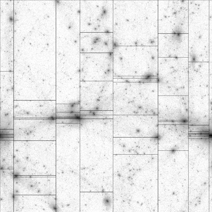
Figure 1: Decomposition in the LCDM universe at $z=0$. It shows 8 $\times$ 8 division in two dimensions.

In our method, we adjust the size of the domains assigned to individual processes, so that the total calculation time of the force (sum of the PP and PM forces) becomes the same for all processes. We use the sampling method (Blackston & Suel, 1997) to determine the geometry of the domains. In its simplest form, each process samples particles with a fixed sampling rate, $R$, and sends them to a process. This process then makes a division, and sends it to all other processes. Finally, each process exchanges particles for all other processes according to the division. This sampling method allows us to drastically reduce the amount of communication that occurs for making a division because a process does not need to know the distribution of all particles.

Table 1: Maximum and minimum numbers of particles and calculation times. $T=t_{\rm pp}+t_{\rm pm}$ for a $1000^{3}$ dark matter simulation with 512 CPU cores at $z=0$.

Correction factor	$N_{i}/N$	Eq. (9)	Eqs. (9) and (10)
$N_{\rm min}$	1941414	1433413	1431633
$N_{\rm max}$	1965026	2548045	2359332
$T_{\rm min}$	29.84	38.07	35.81
$T_{\rm max}$	50.96	40.39	41.18

A naive way to take into account the calculation cost of particles in the sampling method would be the following. The process that makes the domain decomposition collects both the sampled particles and their calculation cost, and determines the geometry of the domains while taking into account the calculation cost. This scheme would work fine, but it is rather complicated. We achieve the same effect not by assigning the cost to the sampled particles, but by changing the sampling rate of the particles according to the calculation cost.

The number of particles, $n_{{\rm samp},i}$, sampled on the $i$-th process is determined as

$$n_{{\rm samp},i}=NR_{\rm samp}f_{{\rm samp},i},$$ (8)

where $N$ is the total number of particles, $R_{\rm samp}$ is the global sampling rate, and $f_{{\rm samp},i}$ is a correction factor needed to achieve a balanced state. We chose $R_{\rm samp}$ so that the cost of the calculation and communication is small, and yet $NR_{\rm samp}/p$, where $p$ is the number of processes, is large enough that the fluctuation due to sampling is small. We typically use $R=4\times 10^{-4}$.

We use the following formula to determine the correction factor:

$$f_{{\rm samp},i}=\frac{t_{{\rm PP},i}+t_{{\rm PM},i}}{\displaystyle\sum_{j}\left(t_{{\rm PP},j}+t_{{\rm PM},j}\right)},$$ (9)

where $t_{{\rm pp},i}$ and $t_{{\rm pm},i}$ are the CPU time for PP and PM part of the $i$-th process, respectively. By this strategy, any imbalance in the CPU time will be corrected. If the calculation on one process takes a time longer than the average, it will sample more particles than average. When the new domain decomposition is created, it is adjusted so that all domains have the same number of sampled particles. Therefore, the size of the domain for this process becomes somewhat smaller, and the CPU time for the next timestep is expected to become smaller.

Figure 1 shows the domain decomposition for a simulation of a LCDM universe at $z=0$. It shows 8 $\times$ 8 division in two dimensions. The total number of particles is $256^{3}$. We can see that high-density regions, such as halo centers are divided into small boxes. In this case, the maximum number of particles in a box is 379569 and the minimum is 189901.

One potential problem of our method, or any method that aims to achieving a good load balance, is the imbalance in the memory usage. Figure 2 shows the cumulative distribution of the number of particles per core, for an Ishiyama et al. (2009) simulation ($N=1600^{3}$, $z=0$, $\theta=0.5$, and $p=2048$) . In this example, the process with the maximum number of particles contains about 50% more particles than average (3035116 compared to 2000000). Therefore, we need 50% more memory to store the particles. Since the memory available to individual MPI processes is usually fixed, we need this 50% more memory for all processes, and for most of processes this additional memory is not used.

If the amount of memory is critical, it is easy to place the upper limit to the number of particles on one process, by placing a lower limit on the number of particles to be sampled given by

$$\underline{\it n}_{{\rm samp},i}=\frac{N_{i}R_{\rm samp}}{1+\alpha},$$ (10)

where $N_{i}$ is the current number of particles in process $i$, and $\alpha$ is a parameter that controls the maximum number of particles for one process. If $n_{{\rm samp},i}$, calculated using equation (8), is smaller than $\underline{\it n}_{{\rm samp},i}$, we use the latter value as the number of particles to be sampled. If we set $\alpha=0.2$, the maximum number of particles in one process is adjusted so that it does not exceed the average value by more than 20%.

One might think that this limit on the number of particles for one process would cause a significant degrade of the performance. In practice, however, the degrade is very small. The reason is the following. When we set the upper limit to the number of particles for one process, particles that would be there need to be redistributed to other processors. The average increase in the number of particles on other processes is given by $f_{\rm over}[\langle N_{\rm over}\rangle-N/p(1+\alpha)]/(1-f_{\rm over})$, where $f_{\rm over}$ is the fraction of processes with the number of particles being more than the specified limit, and $\langle N_{\rm over}\rangle$ is the average number of particles for these processes. We found $f_{\rm over}\sim 0.2$ and $\langle N_{\rm over}\rangle\sim 1.3N/p$ when we chose $\alpha=0.2$, in our large cosmological calculation. Therefore, the increase in the calculation time is less than 2%.

Table 1 gives the maximum and minimum numbers of particles and calculation times, $T=t_{\rm pp}+t_{\rm pm}$, for a $1000^{3}$ dark matter simulation with 512 processes at $z=0$. We used $\alpha=0.2$. We measured them for three different load-balance schemes. The first one (second column) is the simplest one which assigns the same number of particles to all processes. The second one is based on the optimal load-balance scheme of equation (9). The third one is a modified one with equation (10).

We can see that the use of equation (10) reduces the maximum number of particles per process from $2.55\times 10^{6}$ to $2.36\times 10^{6}$. This number is very close to $(1+\alpha)N/p=2.34\times 10^{6}$. On the other hand, the increase in the calculation time is actually less than 2%. Thus, by combining equations (9) and (10), we can achieve close-to-optimal use of both the memory and the CPU time.

Figure 2: Cumulative fraction $F$ of CPU cores as a function of the number of particles per process. Here, $N$ is the number of particles per process, and $N_{\rm im}$ is the number of particles imported from all other processes, respectively.

In figure 2 we also show the distribution of $N+N_{\rm im}$, where $N_{\rm im}$ is the number of particles imported from other processes to construct the global tree. In this case, $N_{\rm im}$ is around one quarter of the average number of particles in one process. However, since $N_{\rm im}$ is proportional to $N^{2/3}$, when we use a large fraction of the memory available for one process, the fraction of the memory used for $N_{\rm im}$ becomes small.

2.3.2 Communication

Inter-process communications occur in four places of the code. In order to achieve a high performance, it is crucial to reduce the communication costs.

First communication occurs in the PM part. In our current implementation, all processes receive the entire grid from all other processors, and the amount of communication for one process is $O(N_{\rm PM}^{3})$. With an optimum implementation of parallel FFT, the amount of communication for one process can be reduced to $O(N_{\rm PM}^{3}/p)$. However, we so far have not tried to use parallel FFT, because we can reduce this part by just making $N_{\rm PM}$ small. A reduction of $N_{\rm PM}$ causes an increase in the calculation cost of the PP part, but it is rather modest because of use of the tree.

Second communication is the exchange of tree information in the PP part. Each process imports tree structures in all other processes as superparticles. The amount of communication depends on many factors, but most importantly on the cutoff radius, the opening parameter for the tree, and the surface area of the domains for processes. Thus, adaptive three-dimensional space decomposition is critical here.

The third one is that for the sampling method. Typically, we can make this much smaller than the rest.

The fourth one is the redistribution of particles after the new domain geometry is determined. In the case of cosmological $N$-body simulations, this part is very small, because the velocity of a particle, relative to the simulation box, is tiny in cosmological simulations.

Thus, the communication of the tree structure is the most expensive. As shown later, in our implementation the time for this part is less than 2% of the time for the PP force calculation, if the number of particles per process is $10^{6}$ or more.

2.4 Softening and Timesteps

Time integration is performed in comoving coordinates. We usually use shared and time-dependent Plummer softening, $\varepsilon(z)$, given by equation (13), which is similar to those used in Kawai et al. (2004) and Kase et al. (2007). It is given by

$$\varepsilon(z)=\left\{\begin{array}[]{r}{\displaystyle\frac{1+z_{\rm crit}}{1+z}\varepsilon_{\rm fin}}\quad(z\geq z_{\rm crit})\vspace{3mm}\\ {\displaystyle\varepsilon_{\rm fin}\quad(z<z_{\rm crit})},\end{array}\right.$$ (13)

where $\varepsilon_{\rm fin}$ is the softening for $z=0$. The softening is constant up to $z=z_{\rm crit}$ in comoving coordinates. After $z=z_{\rm crit}$, it is constant in physical coordinate.

The timestep $\Delta t(z)$ is also shared. It is adaptive and calculated by the following formula:

$$\Delta t(z)=\zeta\min_{i}\left(\sqrt{\frac{\varepsilon(z)}{|{\bf a}_{i}|}}\thinspace,\thinspace\frac{\varepsilon(z)}{|{\bf v}_{i}|}\right),$$ (14)

where $\zeta$ is an accuracy parameter; ${\it\bf v}_{i}$ and ${\it\bf a}_{i}$ are the velocity and acceleration vector of particle $i$. We usually set $\zeta=1.0$ or $\zeta=2.0$.

3 Accuracy and Performance

In this section, we present the result of measurements of the accuracy and performance of our GreeM code. We used LCDM ($\Omega_{0}=0.3$, $\lambda_{0}=0.7$, $h=0.7$, $\sigma_{8}=0.9$) models consisting of $128^{3}$, $256^{3}$, and $512^{3}$ particles for measuring the performance. The box size was 107Mpc for all models. To generate initial particle distributions, we used the GRAFIC package (Bertschinger, 2001).

3.1 Accuracy

In this section, we discuss the accuracy of GreeM. First, we present the numerical accuracy of the Phantom GRAPE library, and then the overall accuracy of the force obtained with GreeM.

3.1.1 Pairwise force error

The Phantom GRAPE library for the force with cutoff uses single-precision numbers to express the position data. Thus, if we simply convert the original double-precision data to single-precision data, the roundoff error after the subtraction ${\bf x}_{j}-{\bf x}_{i}$ can be rather large. Here, ${\bf x}_{i}$ is the position of the point at which the force is evaluated, and ${\bf x}_{j}$ is the position of a particle that exerts the force. In order to reduce the roundoff error, we pass the shifted values, ${\bf x}_{i}-{\bf x}_{g}$ and ${\bf x}_{j}-{\bf x}_{g}$, to the Phantom GRAPE library. Here, ${\bf x}_{g}$ is the position of the center of the particle groups in Barne’s algorithm. By this treatment, we can reduce the roundoff error after subtraction by a factor proportional to the size of the box for the group, which is on the order of $N^{-1/3}$. Without this treatment, the roundoff error of Phantom GRAPE can be dangerously large.

Figure 3 shows the error of the force between two particles as a function of the distance. The error is defined as

$$f_{\rm err}(r)=\frac{|f_{\rm pg}(r)-f(r)|}{|f_{\rm pg}(r)|},$$ (15)

where $f$ and $f_{\rm pg}$ are forces calculated in standard double precision and that calculated with Phantom GRAPE, respectively. We set the cutoff radius, $r_{\rm cut}$, to $5.859375\times 10^{-3}$ and the softening length to $1.953125\times 10^{-5}$. These are typical values we use in actual simulations in which the box size is normalized to unity.

Figure 3: Pairwise force error of Phantom GRAPE. The solid curve shows the force given in equation (1). The black dots show the relative pairwise force error defined in equation (15). The vertical dashed line indicates the value of the force softening.

The particle distributions and calculation procedure mimic that which appear in the tree algorithm with Barnes’ vectorization algorithm. First, we select the position of the center of the origin of the particle groups used in Barnes’ algorithm. For simplicity, we assume that the size of the box is 1/128. This position, ${\bf x}_{g}$, is generated from the uniform distribution within a cube of unit size. We then, generate the position of one particle, ${\bf x}_{i}$, from the uniform distribution within the cube of size 1/128, with the center of the box at ${\bf x}_{g}$. Next, we generate positions of the other particles, ${\bf x}_{j}$, so that the position vector relative to the first particle has a random orientation and the logarithm of the distance follows a uniform distribution between $10^{-6}$ and unity. We generated 256 values for ${\bf x}_{i}$ and 1024 for ${\bf x}_{j}$.

In figure 3 we plot the results of all pairwise force error measurements. When the relative distance is larger than the softening length, the typical relative error is around $10^{-5}$, but it becomes larger for a distance close to unity. This increase is due to the fact that the PP force approaches to zero at the distance unity. If we measure the error relative to the pure $1/r^{2}$ force, there would be no significant increase in the error. When the distance is smaller than the softening length, the relative error is smaller, because in this region the only source of error is rounding of the two position vectors. Thus, the relative error of Phantom GRAPE library is around $10^{-5}$ for the range of the distance that is relevant. This error is much smaller than what is necessary in cosmological $N$-body simulations.

3.1.2 Total force error

In this section we discuss the distribution of the relative error of the total force calculated with the TreePM algorithm used in GreeM. We define the relative force error, $\Delta f_{i}$, of the $i$-th particle as

$$\Delta f_{i}=\frac{|f_{{\rm TreePM},i}-f_{i}|}{|f_{i}|},$$ (16)

where $f_{{\rm TreePM},i}$ and $f_{i}$ are the acceleration of the $i$-th particle calculated by TreePM and the exact force, respectively. In order to estimate the exact force, we used a direct Ewald summation (Ewald, 1921; Hernquist et al., 1991). The scale length of the Gaussian function used in the Ewald method is 0.1, the real-space cutoff is 0.2, and the wavenumber cutoff is 7.14.

With Phantom GRAPE, we use the interaction list method (Barnes, 1990) to reduce the cost of tree traversal. We use $N_{\rm crit}=300$ as the criterion for the grouping of particles. With this criterion, the average number of particles that share the same interaction list is $\approx N_{\rm crit}/4$ (Makino, 1991).

When we construct the tree, we stop the subdivision of a node if the number of particles in that node is less than $N_{\rm leaf}$. By this method, we can reduced the amount of memory required to store the tree and to reduce the CPU time for tree construction. However, a very large value of $N_{\rm leaf}$ causes an increase in the CPU time for the PP force calculation. For the timing benchmarks, we used $N_{\rm leaf}=10$. The number of particles used here is $128^{3}$.

Figure 4 shows the cumulative distribution of the relative error. The top, middle, and bottom rows show the results with $N_{\rm PM}=64$, 32 and 16, and the left, middle, and right panels in one row show the results at $z=27$, 10, and 0, respectively. In each panel, results with $\theta=0.3$, 0.5 and 1.0 are shown.

The relationship between the accuracy of the force and the accuracy of the result is not well understood. Here, we use the condition that the error of 90% of the particles is less than 2%, which is probably too stringent.

For $N_{\rm PM}=64$, we can achieve this goal with $\theta=0.5$, even at $z=27$, and in the case of $N_{\rm PM}=32$ with $\theta=0.3$. With $N_{\rm PM}=16$, at $z=27$ we would need $\theta=0.2$. For lower values of $z$, we can use a significantly larger $\theta$.

These behaviors of errors are quantitatively in fair agreement with those in previous studies (Bagla, 2002; Wadsley et al., 2004). For a similar choice of parameters, the error of the Gasoline code (Wadsley et al., 2004) seems to be somewhat larger than that of ours. This could be due to the difference in the distribution of particles. However, since they use the Ewald method, the cutoff length of the real-space PP force is much larger than what we used. This difference in the cutoff length might be the cause of the difference between our result and that of Gasoline.

Note that in the case of $N_{\rm PM}=64$, the error is almost the same for $\theta=0.3$ and 0.5 for all values of $z$. Also, for the case of $z=0$, the error is almost the same for $\theta=0.3$ and 0.5. This means that for these cases the error is dominated by a mismatch between the PM force and the PP force.

Figure 4: Cumulative distributions of the relative force errors for $N=128^{3}$ model. Top, middle, and bottom rows show the results with $N_{\rm PM}=64$, 32 and 16. Within each row, the left, center, and right panels show the result at $z=27$, 10 and 0. The solid, dashed, and dotted curves in each panel show the result with $\theta=0.3$, 0.5 and 1.0.

From the point of view of the performance, it is desirable to use a smaller $N_{\rm PM}$, since that would reduce the memory requirement, the amount of communication, and the calculation cost of FFT. However, as we can see from figure 4, the error, especially at high-$z$, increases rapidly as we reduce $N_{\rm PM}$.

Figure 5 and 6 show the error at 90% of the particles as functions of $\theta$ and $N_{\rm PM}$, respectively. We can see that the error at $z=27$ is roughly proportional to $\theta^{2}$ and $N_{\rm PM}^{-1}$. This behavior can be understood as follows.

Figure 5: Error of 90% of the particles as a function of $\theta$. The solid and dashed curves show the results at $z=27$ and $z=0$, respectively. The triangles, squares, and circles show the results with $N_{\rm PM}=16$, 32 and 64, respectively.

Figure 6: Error of 90% of the particles as a function of $N_{\rm PM}$. The solid and dashed curves show the results at $z=27$ and $z=0$, respectively. The triangles, squares, and circles show the results with $\theta=1.0$, 0.5 and 0.3, respectively.

Consider the extreme case of a purely uniform distribution of mass without any density perturbation. In this case, the exact force is zero, and therefore we cannot define the relative error. However, we can still discuss the absolute error.

The error of the force from a single tree node with mass $m$ and size $l$ at distance $r$ is dominated by the second-order (quadrupole) term, since we use the center-of-mass approximation. In the case of a pure $1/r$ potential, the quadrupole term vanishes in the limit of uniform density (Barnes & Hut, 1989), but in the case of the force with cutoff the second-order term does not vanish, and this is the leading error term. Thus, the absolute amount of the error of the force from one node is proportional to $mr^{-2}g_{\rm P3M}(r/\eta)(l/r)^{2}$. If we assume a uniform density of $\rho$, $m\sim\rho l^{3}$, and for a given opening angle we have $l\sim r\theta$. Therefore, the error of the force from a node at distance $r$ is proportional to $\rho r\theta^{5}g(r/\eta)$. We can see that the error is largest at $r\sim\eta$. The number of tree nodes with $r\sim\eta$ is proportional to $\theta^{-3}$, and we cannot assume that the errors from different cells are random, since all cells essentially have the same second-order terms. Therefore, the total error is proportional to $\rho\eta\theta^{2}$.

We conclude that if we are to use a large PM grid spacing (more than $4H$), the opening angle should be set to be less than 0.3 from initial to $z=10$. From $z=10$, we can use the opening angle around 0.5. If we use a small PM grid spacing (less than $2H$), the opening angle should be set to be less than 0.5 from initial to $z=10$.

3.2 Performance

In this section we report on the measured performance of GreeM. We used a Cray XT4 at Center for Computational Astrophysics (CfCA), National Astronomical Observatory of Japan for the measurement. It consists of 740 Opteron quad-core processors at a clock speed of 2.2 GHz (the total number of cores is 2960) and 5.7TB of memory. The peak performance is 26 Tflops. Processors are connected in a 3D torus network with the Cray SeaStar2 chip. The peak bandwidth of a single link of the torus network is about 7.6Gbyte/sec.

First, we present a result of the measurement of the parallel performance (scaling of the performance). We then go into the details, such as a breakdown of the CPU time, the dependence on the opening angle, that on the distribution of particles, and memory usage.

3.2.1 Scalability

For measuring of the scalability, we used $256^{3}$, $512^{3}$ and $1000^{3}$ particles, and $N_{\rm PM}=N^{1/3}/2$. For $1000^{3}$ particles, we used $N_{\rm PM}=N^{1/3}/4$, to save the memory for the PM grid. We measured the CPU time at $z=0$. The parameters of the tree parts were $\theta=0.5$, $N_{\rm crit}=300$, and $N_{\rm leaf}=10$.

Figure 7 shows the CPU time per step as a function of the number of CPU cores. In the case of $256^{3}$ particles, the parallel speedup is almost perfect for up to 64 cores, and even with 256 cores the gain is good. For $512^{3}$ particles, parallel speedup is fine with up to 256 cores, but degrades with more cores. With $1000^{3}$ particles, parallel speedup is almost perfect for the maximum number of cores we used for the test (1024 cores).

The leveling-off of the parallel speedup comes from a leveling-off of the CPU time of the PM part. As discussed earlier, the time for communication and the FFT operation of the PM part is independent of the number of cores, since these parts are not parallelized. Thus, for a large number of cores, the CPU time for these parts starts to limit the speedup. For $256^{3}$ and $512^{3}$ particles, the ratio between the total number of particles and the total number of PM grid points is the same. Thus, the dependence of the parallel speedup on the number of cores is also roughly the same. In the case of $1000^{3}$ particles, we reduced the number of PM grids, which is the reason why the parallel speedup became improved. As discussed in subsection 3.1.2, the error of the calculated gravitational force is proportional to the inverse of the grid point. Therefore, when we use a small PM grid, we should use a small opening angle for the tree part to retain accuracy. This choice might result in an increase of the total CPU time, even though the parallel speedup is improved.

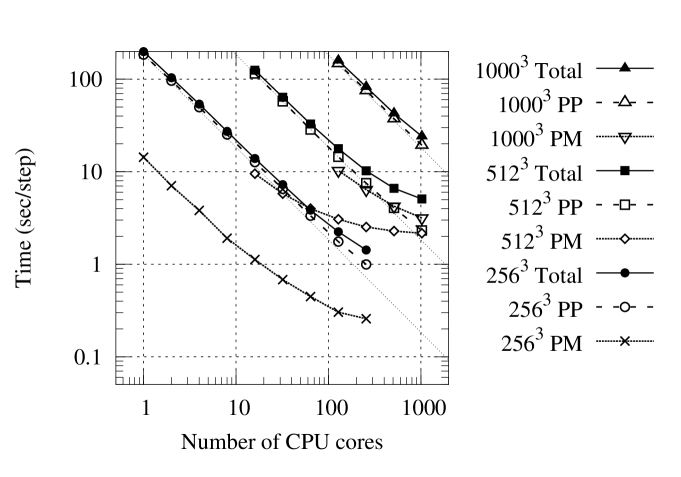
Figure 7: Calculation time per step of our code as a function of the number of CPU cores on Cray-XT4. The curves with filled triangles, squares and circles show the results for total calculation time of $1000^{3}$, $512^{3}$, and $256^{3}$ dark matter simulations, respectively. The curves with open triangles, squares and circles show the results for the PP part, respectively. The curves with open inverted triangles, argyles and crosses show the results for the PM part, respectively.

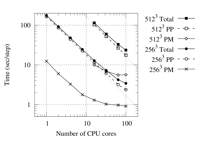
Figure 8: Calculation time per step as a function of the number of CPU cores on a PC cluster with Gigabit Ethernet. The curves with filled squares and circles show the results for total calculation time of $512^{3}$, and $256^{3}$ dark matter simulations, respectively. The curves with open squares and circles show the results for the PP part, respectively. The curves with open argyles and crosses show the results for the PM part, respectively.

Figure 8 shows the parallel speedup on a PC cluster of 25 nodes connected with Gigabit Ethernet. Each node has one Intel Core2 Quad processor (2.4GHz Q6600) and 8GB of PC6400 memory. We can see that the speed of a PC cluster is quite similar to that of the Cray XT4 with the same number of cores, except that the time for the PM part is significantly longer when the number of CPU cores is more than 32. For 100 cores, our PC cluster is about three-times slower than the Cray XT4, while the speed of the PP part is almost the same for all values of the number of particles and the number of processes. This difference comes from the difference in the speed of the network. If we use $N_{\rm PM}=N^{1/3}/4$, even with a slow Gigabit Ethernet, we can probably use 1024 cores without seeing any significant loss of efficiency.

3.2.2 Calculation Cost

Table 2 gives a breakdown of the calculation cost per step. We used a run with $512^{3}$ dark matter particles for a measurement of the performance. We used a snapshot at $z=0$ to measure the CPU time for a single timestep. The number of grid points for the PM calculation in one dimension was $N_{\rm PM}=256$. The parameters of the tree parts were $\theta=0.5$, $N_{\rm crit}=300$, and $N_{\rm leaf}=10$. The sampling parameter was $R_{\rm samp}=4.0\times 10^{-4}$. This means that $NR_{\rm samp}=53687$ particles were sampled for the domain update. Here, $p$ is the number of CPU cores.

Table 2: Calculation time per step of our code.

$p$	16	128	1024
$N/p$	8388608	1048576	131072
PM (s/step)	9.72	2.93	1.99
density assignment	1.59	0.28	0.10
comm	0.58	0.50	0.50
FFT	1.12	1.17	1.17
convolution	0.10	0.10	0.10
force interpolation	6.33	0.88	0.12
PP (s/step)	110.8	13.76	1.93
local tree	3.38	0.38	0.062
comm	1.12	0.25	0.19
tree construction	2.75	0.35	0.058
tree traversal	30.42	3.92	0.44
force calculation	73.13	8.86	1.14
Others (s/step)	1.45	0.65	0.64
position update	0.20	0.003	0.00045
sampling method	0.46	0.08	0.03
exchange	0.05	0.027	0.028
synchronization	0.74	0.54	0.58
Total (s/step)	121.97	17.34	4.56

In our current implementation, all processes have the same PM grid, and FFT of the entire region is duplicated in all processes. Therefore, both the communication and calculation require the time to be independent of the number of cores. An obvious way to improve the performance of this part is to use parallel FFT, such as the MPI version of the FFTW library. We have not implemented this, but might consider to do so in future since the use of larger values of $N_{\rm PM}$ allows us to use a larger opening angle, resulting in a reduction of the CPU time for the PP part.

3.2.3 Dependence on the Opening Angle

Figure 9 shows the CPU time per step and the average number of force interactions, $N_{\rm int}$, per particle as functions of the opening angle. We used $512^{3}$ simulations on 32 processors with 128 CPU cores. The parameters of the tree parts were $N_{\rm crit}=300$ and $N_{\rm leaf}=10$.

We can see that for small values of $\theta$, $N_{\rm int}$ is roughly proportional to $\theta^{-2}$. Since the CPU time is dominated by the time for the PP part, it shows almost the same behavior as $N_{\rm int}$. For $\theta>0.75$, the dependence of $N_{\rm int}$ on $\theta$ is weak, because in this regime $N_{\rm int}$ is determined by $N_{\rm crit}$ and $N_{\rm leaf}$ (Makino, 1991).

Figure 9: Dependence on the opening angle of the calculation time per step (top) and the number of force interactions per particle, $N_{\rm int}$ (bottom), for $512^{3}$ dark matter simulation. The number of CPU cores for the calculations is 128. The number of force interactions per particle of the first process is plotted.

For $\theta=0.5$, the average, minimum, and maximum of $N_{\rm int}$ are 2116, 1510, and 3156, respectively. On the other hand, those of the time for the PP part are 13.97, 13.61, 14.56, respectively. We can see that the balance of the CPU time between teh processes is very good, with only a 4% difference between the average and the maximum. This means that the loss of the performance due to non-optimal load balancing is around 4%.

We have not investigated the cause of this variation of the time for the PP force, but the most likely reason is fluctuation due to sampling, since we sample only about 400 particles per process.

3.2.4 Dependence on the particle distribution

Figure 10 shows the CPU time per step, the amount of data transferred, $D$, and the number of force interactions, $N_{\rm int}$, as functions of the redshift. We used $512^{3}$ simulations on 32 processors with 128 CPU cores. Other parameters for the tree parts were $\theta=0.5$, $N_{\rm crit}=300$, and $N_{\rm leaf}=10$. The amount of data transferred, $D$, is given by

$$D=16N_{\rm im}{\rm bytes},$$ (17)

where $N_{\rm im}$ is the number of particles imported from all other processes in the PP part. We consider only the communication for the tree construction. One particle consists of the three-dimensional position and the mass, and the amount of data is 16 bytes per particle. The communication for the PM grid is independent of the particle distribution, and the amount of data transfer is 64MB per timestep. Others are all small compared to the tree construction.

Figure 10: Dependence on the redshift of the calculation time per step (top), the amount of data transferred, $D$ (middle), and the number of force interactions per particle $N_{\rm int}$ (bottom) for $512^{3}$ dark matter simulation. The number of CPU cores for the calculations was 128. The calculation time and number of force interactions per particle and $D$ of first process are plotted. We measured the amount of data transferred of only the PP part.

The calculation time is nearly constant from the start of the calculation until $z=4$, and increases slowly afterwards as the degree of clustering becomes higher. This increase is due to the increase of $N_{\rm int}$.

The amount of communication, $D$, decreases as the clustering proceeds, because of the formation of low-density voids. Since we use the tree algorithm, the formation of high-density regions does not significantly increase the amount of communication, while the communication need of low-density regions is lower because of the cutoff distance of the interaction. As a result, with TreePM, the amount of communication decreases as the clustering proceeds. This behavior is opposite to that of the ${\rm P^{3}M}$ scheme, with which the communication increases as the clustering proceeds.

3.2.5 Memory requirement

The amount of required memory per particle is 48 bytes. We need to store the position (three double precision words), the velocity (three single precision words), a unique ID (one 64-bit integer word), and the mass (one single precision word). The memory requirement per tree node is 52 bytes. The number of nodes per particle is $\min(1,7.5/N_{\rm leaf})$. In addition, another 12 bytes are required per particle for the tree-force calculation in order to generate the morton key. Thus the total amount of memory, $M$, required per particle is given by the following formula:

$$M=60+52\cdot\min\left(1\thinspace,\thinspace\frac{7.5}{N_{\rm leaf}}\right){\rm bytes}.$$ (18)

The amount of memory per PM grid point is 4.5 bytes. It includes the mass density (one single precision word) and the green function table. The green function table also needs one single precision word per table. The number of tables is $(1/8)N_{\rm PM}^{3}$ owing to periodicity. This amount is needed in all nodes.

We can use the same memory area to store the PM grid and the tree structure, since they are not used at the same time, and both of them are constructed from scratch at each timestep.

As discussed in subsection 2.3.1, our optimal load balance algorithm can cause a significant imbalance in the memory usage of up to a factor of two. However, as we have already shown, we can reduce the additional amount of memory required to around 20% or less of the total amount of memory for particles, without any significant degradation in performance.

4 Discussion and Summary

4.1 Possible Ways to Improve Accuracy

As we have shown in subsection 3.1, the total force error of the TreePM method is dominated by the error of the forces from tree nodes at a distance of around $\eta$. Thus, one possibility of reducing the error is to use distance-dependent opening criterion (Makino, 1991). Since the error in the limit of the uniform density distribution is proportional to $r\theta^{2}g(r/\eta)$, if we set

$$\theta=\frac{\theta_{0}}{\sqrt{rg(r/\eta)}},$$ (19)

the error is evenly distributed over all nodes, and thus the error should be minimized. It is probably necessary to set some upper-limit value, since with the above criterion alone $\theta$ would diverge at both ends of $r$.

A more natural approach is to include higher-order terms of expansion. Note that the multipole expansion of force with cutoff is different from that of a pure $1/r$ force, and should include the spacial derivatives of the cutoff function. Thus, its implementation differs from the usual high-order multipole moment. The second-order moment is fairly easy to implement, and can drastically improve the accuracy.

4.2 Comparison with Another Code

Here, we compare the performance of GreeM with that of GADGET-2 (Springel, 2005). We discuss only the scalability, because the comparison of the absolute speed does not have much meaning if the hardware used is different. We used the data of figure 19 in Springel (2005) for a $270^{3}$ dark matter simulation. We used a $256^{3}$ dark matter simulation for GreeM. This comparison is not an exact one since the dark matter distributions and computers were different. However it should give us some useful information.

Figure 11: Speed up of our code and GADGET-2 plotted against the number of CPU cores. The filled circles and open squares show the result of GreeM and that of GADGET-2, respectively [figure 19 in Springel (2005)].

Figure 11 shows the speed-up factors of our code and GADGET-2 as a function of the number of CPU cores. We can see that the scaling of GreeM is better than that of GADGET-2. The most likely reason for this difference is the difference in the load balance. Even for a very small number of processes, the load imbalance of GADGET-2 is large (as can be seen in their table 1). We achieved a nearly perfect load balance, for an arbitrary number of processes.

4.3 Summary

In this paper, we described our new cosmological N-body simulation code, GreeM, which uses the TreePM algorithm, and is optimized for large parallel systems. GreeM achieves a nearly perfect load balance, even for a very large number of cores, resulting in very good scalability.

GreeM runs efficiently on PC clusters, but the scalability is naturally better on parallel computers with high-speed networks. The measured calculation speed on the Cray XT4 is $5\times 10^{4}$ particles per second per CPU core, if the number of particles per CPU core is larger than $5\times 10^{5}$. On a cluster of PCs with quad-core CPU and GbE network, GreeM achieves a similar speed if the number of particles per core is more than $3\times 10^{6}$. Using this code, we have already performed $1600^{3}$ dark matter simulation on Cray-XT4 (Ishiyama et al., 2009). It spent about 0.6 million CPU hours.

We are grateful to Kohji Yoshikawa for providing his parallel TreePM code. We thank Keigo Nitadori for his technical advices and providing his Phantom GRAPE code. T.I. thanks Simon Portegies Zwart and Derek Groen for helpful discussions and advices. Numerical computations were carried out on a Cray XT4 and a PC cluster at Center for Computational Astrophysics, CfCA, of National Astronomical Observatory of Japan. T.I. is financially supported by a Research Fellowship of the Japan Society for the Promotion of Science (JSPS) for Young Scientists. This research is partially supported by the Special Coordination Fund for Promoting Science and Technology (GRAPE-DR project), Ministry of Education, Culture, Sports, Science and Technology, Japan.

References

- Bagla (2002) Bagla, J. S. 2002, Journal of Astrophysics and Astronomy, 23, 185
- Barnes & Hut (1986) Barnes, J., & Hut, P. 1986, Nature, 324, 446
- Barnes & Hut (1989) Barnes, J. E., & Hut, P. 1989, ApJS, 70, 389
- Barnes (1990) Barnes, J. E. 1990, Journal of Computational Physics, 87, 161
- Bertschinger (2001) Bertschinger, E. 2001, ApJS, 137, 1
- Blackston & Suel (1997) Blackston, D., & Suel, T. 1997, Proc.SC97
- Bode et al. (2000) Bode, P., Ostriker, J. P., & Xu, G. 2000, ApJS, 128, 561
- Bode & Ostriker (2003) Bode, P., & Ostriker, J. P. 2003, ApJS, 145, 1
- Couchman (1991) Couchman, H. M. P. 1991, ApJ, 368, L23
- Dubinski (1996) Dubinski, J. 1996, New Astronomy, 1, 133
- Dubinski et al. (2004) Dubinski, J., Kim, J., Park, C., & Humble, R. 2004, New Astronomy, 9, 111
- Ewald (1921) Ewald, P. P. 1921, Annalen der Physik, 369, 253
- Fukushige et al. (2005) Fukushige, T., Makino, J., & Kawai, A. 2005, PASJ, 57, 1009
- Hernquist et al. (1991) Hernquist, L., Bouchet, F. R., & Suto, Y. 1991, ApJS, 75, 231
- Hockney & Eastwood (1981) Hockney, R. W., & Eastwood, J. W. 1981, Computer Simulation Using Particles, New York: McGraw-Hill, 1981,
- Ishiyama et al. (2009) Ishiyama, T., Fukushige, T., & Makino, J. 2009, ApJ, 696, 2115
- Kase et al. (2007) Kase, H., Makino, J., & Funato, Y. 2007, PASJ, 59, 1071
- Kawai et al. (2000) Kawai, A., Fukushige, T., Makino, J., & Taiji, M. 2000, PASJ, 52, 659
- Kawai et al. (2004) Kawai, A., Makino, J., & Ebisuzaki, T. 2004, ApJS, 151, 13
- Khandai & Bagla (2009) Khandai, N., & Bagla, J. S. 2009, Research in Astronomy and Astrophysics, 9, 861
- Makino (1991) Makino, J. 1991, PASJ, 43, 621
- Makino & Taiji (1998) Makino, J., & Taiji, M. 1998, Scientific Simulations with Special-Purpose Computers : The GRAPE Systems (Chichester : John Wiley & Sons)
- Makino et al. (2003) Makino, J., Fukushige, T., Koga, M., & Namura, K. 2003, PASJ, 55, 1163
- Makino (2004) Makino, J. 2004, PASJ, 56, 521
- Nitadori et al. (2006) Nitadori, K., Makino, J., & Hut, P. 2006, New Astronomy, 12, 169
- Peacock (1999) Peacock, J. A. 1999, Cosmological Physics, by John A. Peacock, pp. 704. ISBN 052141072X. Cambridge, UK: Cambridge University Press, January 1999.,
- Springel (2005) Springel, V. 2005, MNRAS, 364, 1105
- Sugimoto et al. (1990) Sugimoto, D., Chikada, Y., Makino, J., Ito, T., Ebisuzaki, T., & Umemura, M. 1990, Nature, 345, 33
- Wadsley et al. (2004) Wadsley, J. W., Stadel, J., & Quinn, T. 2004, New Astronomy, 9, 137
- Warren & Salmon (1992) Warren, M. S. and Salmon, J. K. 1992, Supercomputing ’92: Proceedings of the 1992 ACM/IEEE conference on Supercomputing
- Warren & Salmon (1993) Warren, M. S. and Salmon, J. K. 1993, Supercomputing ’93: Proceedings of the 1993 ACM/IEEE conference on Supercomputing
- White & Rees (1978) White, S. D. M., & Rees, M. J. 1978, MNRAS, 183, 341
- Xu (1995) Xu, G. 1995, ApJS, 98, 355