Expectation Propagation on the Maximum
of Correlated Normal Variables

Abstract

Many inference problems involving questions of optimality ask for the maximum or the minimum of a finite set of unknown quantities. This technical report derives the first two posterior moments of the maximum of two correlated Gaussian variables and the first two posterior moments of the two generating variables (corresponding to Gaussian approximations minimizing relative entropy). It is shown how this can be used to build a heuristic approximation to the maximum relationship over a finite set of Gaussian variables, allowing approximate inference by Expectation Propagation on such quantities.

1 Introduction

Many optimization problems involve inference on the maximum or minimum of a set of variables. This very broad class includes shortest path problems (Burton and Toint, 1992), Reinforcement Learning (Dearden et al., 1998), and scientific inference in Seismology (Neumann-Denzau and Behrens, 1984), to name but a few. Often, there is a corresponding inverse optimization problem (Ahuja and Orlin, 2001; Heuberger, 2004), where the optimal solution is known with some uncertainty and the question is about the quantities generating this optimum. Most contemporary algorithms for this case aim to provide a point estimate (typically the least-squares solution), but have trouble offering an error estimate on this estimate as well.

This work derives (Section 2) mean and variance of the posterior of the maximum of two correlated Gaussian variables (for forward optimization problems), and the mean and variance on the posterior of the Gaussian variables generating the maximum (for inverse optimization problems). These two moments correspond to the approximation within the exponential family of Gaussian distributions minimizing the Kullback-Leibler Divergence (relative entropy) to the true posterior. It will be shown how these results can be used to build a heuristic approximation to the max of a finite set of normal variables (Section 3). Together, this provides the necessary results for Expectation Propagation (Minka, 2001) on graphs involving the “max” relationship. Because maximum and minimum obey the simple relationship $\max(\{x_{i}\})=-\min(\{-x_{i}\})$, this also allows inference on the minimum where necessary. Limitations of this approximation are examined in Section 4.

The moments of the normalized likelihood function of the maximum of two normal variables have previously been derived by Clark (1961). To my best knowledge, this is the first publication deriving the full posterior, and the first to report the posterior for the inverse problem (see also Section 2.4.3).

2 The Maximum of Two Gaussian Variables

2.1 Notation

We consider two normally distributed variables $x_{1}$ and $x_{2}$, forming the vector $\boldsymbol{x}$. Let there be some prior (i.e. outside) information $\mathfrak{I}_{\mathfrak{g}}$ giving rise to the belief

$$p(x_{1},x_{2}|\mathfrak{I}_{\mathfrak{g}}) =\mathcal{N}(\boldsymbol{x};\boldsymbol{\mu}_{\mathfrak{g}},\boldsymbol{\Sigma}_{\mathfrak{g}})=\frac{1}{2\pi\sigma_{\mathfrak{g}1}\sigma_{\mathfrak{g}2}(1-\rho^{2})^{1/2}}\exp\left(-\frac{1}{2}(\boldsymbol{x}-\boldsymbol{\mu}_{\mathfrak{g}})^{\text{T}}\boldsymbol{\Sigma}_{\mathfrak{g}}^{-1}(\boldsymbol{x}-\boldsymbol{\mu}_{\mathfrak{g}})\right)$$ (1)

over their values. Here we have defined a mean vector $\boldsymbol{\mu}_{\mathfrak{g}}=(\mu_{\mathfrak{g}1},\mu_{\mathfrak{g}2})^{\text{T}}$ and a covariance matrix $\boldsymbol{\Sigma}_{\mathfrak{g}}$. The latter has the form

$$\boldsymbol{\Sigma}_{\mathfrak{g}}=\begin{pmatrix}\sigma_{\mathfrak{g}1}^{2}&\rho\sigma_{\mathfrak{g}1}\sigma_{\mathfrak{g}2}\\ \rho\sigma_{\mathfrak{g}1}\sigma_{\mathfrak{g}2}&\sigma_{\mathfrak{g}2}^{2}\end{pmatrix}\qquad\text{and thus}\qquad\boldsymbol{\Sigma}_{\mathfrak{g}}^{-1}=\frac{1}{\sigma_{\mathfrak{g}1}^{2}\sigma_{\mathfrak{g}2}^{2}(1-\rho^{2})}\begin{pmatrix}\sigma_{\mathfrak{g}2}^{2}&-\rho\sigma_{\mathfrak{g}1}\sigma_{\mathfrak{g}2}\\ -\rho\sigma_{\mathfrak{g}1}\sigma_{\mathfrak{g}2}&\sigma_{\mathfrak{g}1}^{2}\end{pmatrix}$$ (2)

with the linear coefficient of correlation

$$\rho=\frac{\operatorname{cov}(x_{1},x_{2})}{\sigma_{\mathfrak{g}1}\sigma_{\mathfrak{g}2}}$$ (3)

(for notational convenience, the index $\mathfrak{g}$ is dropped from $\rho$ because there will be no chance for confusion). We further introduce the variable $m$ which is defined through $m=\max(x_{1},x_{2})$, and we assume that there is some outside prior information $\mathfrak{I}_{\mathfrak{m}}$ on the value of $m$ as well:

$$p(m|\mathfrak{I}_{\mathfrak{m}})=\mathcal{N}(m;\mu_{\mathfrak{m}},\sigma_{\mathfrak{m}}^{2})$$ (4)

The inference problems to be solved are

• The posterior over $m$ given both $\mathfrak{I}_{\mathfrak{m}}$ and $\mathfrak{I}_{\mathfrak{g}}$ (jointly called $\mathfrak{I}_{\mathfrak{c}}$):

  $$p(m|\mathfrak{I}_{\mathfrak{c}})=\frac{p(m|\mathfrak{I}_{\mathfrak{m}})\int p(\boldsymbol{x}|m)p(\boldsymbol{x}|\mathfrak{I}_{\mathfrak{g}})\operatorname{d}\!\boldsymbol{x}}{\int\left[p(m|\mathfrak{I}_{\mathfrak{m}})\int p(\boldsymbol{x}|m)p(\boldsymbol{x}|\mathfrak{I}_{\mathfrak{g}})\operatorname{d}\!\boldsymbol{x}\right]\operatorname{d}\!m}=Z^{-1}p(m|\mathfrak{I}_{\mathfrak{m}})\int p(\boldsymbol{x}|m)p(\boldsymbol{x}|\mathfrak{I}_{\mathfrak{g}})\operatorname{d}\!\boldsymbol{x}$$ (5)

  with the normalization constant $Z=\iint p(\boldsymbol{x},m|\mathfrak{I}_{\mathfrak{c}})\operatorname{d}\!\boldsymbol{x}\operatorname{d}\!m$. This problem will be called the “forward” problem here.

• The posterior over $\boldsymbol{x}$ given $\mathfrak{I}_{\mathfrak{c}}$,

  $$p(\boldsymbol{x}|\mathfrak{I}_{\mathfrak{c}})=\frac{p(\boldsymbol{x}|\mathfrak{I}_{\mathfrak{g}})\int p(m|\boldsymbol{x})p(m|\mathfrak{I}_{\mathfrak{m}})\operatorname{d}\!m}{\int\left[p(\boldsymbol{x}|\mathfrak{I}_{\mathfrak{g}})\int p(\boldsymbol{x}|m)p(m|\mathfrak{I}_{\mathfrak{m}})\operatorname{d}\!m\right]\operatorname{d}\!\boldsymbol{x}}=Z^{-1}p(\boldsymbol{x}|\mathfrak{I}_{\mathfrak{g}})\int p(m|\boldsymbol{x})p(m|\mathfrak{I}_{\mathfrak{m}})\operatorname{d}\!m$$ (6)

  This problem will be called the “inverse” problem.

Throughout the derivations, the notation

$$\mathcal{N}(x;\mu,\sigma^{2}) \equiv\frac{1}{\sqrt{2\pi\sigma^{2}}}\exp\left[-\frac{1}{2}\left(\frac{x-\mu}{\sigma}\right)^{2}\right]$$ (7)

$$\phi(x) \equiv\frac{1}{\sqrt{2\pi}}\exp\left(-\frac{x^{2}}{2}\right)$$

$$\Phi(x) \equiv\int_{-\infty}^{x}\phi(t)\operatorname{d}\!t=\frac{1}{2}\left[1+\operatorname{erf}\left(\frac{x}{\sqrt{2}}\right)\right]$$

will be used to denote the general and standard normal probability density functions (PDF) and the standard normal cumulative distribution function (CDF).

2.2 Some Integrals

The derivations in this paper will repeatedly feature certain integrals. The first two incomplete moments of the standard Gaussian are

$$\int_{-\infty}^{y}t\phi(t)\operatorname{d}\!t =-\phi(y)$$ (8)

$$\int_{-\infty}^{y}t^{2}\phi(t)\operatorname{d}\!t =\Phi(y)-y\phi(y)$$

this is obvious directly from differentiation. A simple substitution gives

$$\int_{-\infty}^{y}t\mathcal{N}(t;\alpha,\beta^{2})\operatorname{d}\!t = \alpha \Phi\left(\frac{y-\alpha}{\beta}\right)- \beta \phi\left(\frac{y-\alpha}{\beta}\right)$$ (9)

$$\int_{-\infty}^{y}t^{2}\mathcal{N}(t;\alpha,\beta^{2})\operatorname{d}\!t = (\alpha^{2}+\beta^{2}) \Phi\left(\frac{y-\alpha}{\beta}\right)- (\alpha+y)\beta \phi\left(\frac{y-\alpha}{\beta}\right)$$ (10)

Further, we will use the integrals

$$\int_{-\infty}^{\infty}\Phi\left(\frac{x-a}{b}\right)\mathcal{N}(x;\alpha,\beta^{2})\operatorname{d}\!x =\Phi(z)$$ (11)

$$\int_{-\infty}^{\infty}x\Phi\left(\frac{x-a}{b}\right)\mathcal{N}(x;\alpha,\beta^{2})\operatorname{d}\!x =\alpha\Phi(z)+\frac{\beta^{2}}{b\sqrt{1+\beta^{2}/b^{2}}}\phi(z)$$

$$\int_{-\infty}^{\infty}x^{2}\Phi\left(\frac{x-a}{b}\right)\mathcal{N}(x;\alpha,\beta^{2})\operatorname{d}\!x =(\alpha^{2}+\beta^{2})\Phi(z)+\left[2\alpha\frac{\beta^{2}}{b\sqrt{1+\beta^{2}/b^{2}}}-z\frac{\beta^{4}}{b^{2}+\beta^{2}}\right]\phi(z)$$

$$\text{where}\qquad z =\frac{\alpha-a}{b\sqrt{1+\beta^{2}/b^{2}}}$$

A derivation of these results can, for example, be found in Rasmussen and Williams (2006, section 3.9)

2.3 Analytic Forms

2.3.1 Forward Problem

Neither of the posterior distributions are normal themselves. The forward posterior is

$$p(m|\mathfrak{I}_{\mathfrak{c}}) =Z^{-1}p(m|\mathfrak{I}_{\mathfrak{m}})\iint_{-\infty}^{\infty}p(\boldsymbol{x}|m)p(\boldsymbol{x}|\mathfrak{I}_{\mathfrak{g}})\operatorname{d}\!\boldsymbol{x}$$ (12)

$$=Z^{-1}p(m|\mathfrak{I}_{\mathfrak{m}})\int_{-\infty}^{\infty}\left[\int_{-\infty}^{x_{1}}\delta(x_{1}-m)p(\boldsymbol{x}|\mathfrak{I}_{\mathfrak{g}})\operatorname{d}\!x_{2}+\int_{x_{1}}^{\infty}\delta(x_{2}-m)p(\boldsymbol{x}|\mathfrak{I}_{\mathfrak{g}})\operatorname{d}\!x_{2}\right]\operatorname{d}\!x_{1}$$

$$=Z^{-1}\mathop{\underbrace{p(m|\mathfrak{I}_{\mathfrak{m}})\int_{-\infty}^{\infty}\delta(x_{1}-m)\int_{-\infty}^{x_{1}}p(\boldsymbol{x}|\mathfrak{I}_{\mathfrak{g}})\operatorname{d}\!x_{2}\operatorname{d}\!x_{1}}}_{\nu_{1}}$$

$$\quad+Z^{-1}\mathop{\underbrace{p(m|\mathfrak{I}_{\mathfrak{m}})\int_{-\infty}^{\infty}\delta(x_{2}-m)\int_{-\infty}^{x_{2}}p(\boldsymbol{x}|\mathfrak{I}_{\mathfrak{g}})\operatorname{d}\!x_{1}\operatorname{d}\!x_{2}}}_{\nu_{2}}$$

For a motivation of the change in the integration ranges from the second to the third line in Equation (12), consider the sketch in Figure 1.

Figure 1: Sketch of the integration range for $\nu_{2}$. The open set $(x_{1},x_{2})\in((-\infty,\infty),(x_{1},\infty))$ is identical to the open set $(x_{1},x_{2})\in((-\infty,x_{2}),(-\infty,\infty))$.

Since the two summands are related to each other through the symmetry $x_{1}\leftrightarrow x_{2}$, consider only the first term, $\nu_{1}$. To solve the integrals, note that the bi-variate Gaussian $p(\boldsymbol{x}|\mathfrak{I}_{\mathfrak{g}})$ can be re-written as

$$p(x_{1},x_{2}|\mathfrak{I}_{\mathfrak{g}}) =p(x_{1}|\mathfrak{I}_{\mathfrak{g}})p(x_{2}|x_{1},\mathfrak{I}_{\mathfrak{g}})$$ (13)

$$=\frac{1}{\sqrt{2\pi\sigma_{\mathfrak{g}1}^{2}}}\exp\left[-\frac{1}{2}\left(\frac{x_{1}-\mu_{\mathfrak{g}1}}{\sigma_{\mathfrak{g}1}}\right)^{2}\right]$$

$$\quad\frac{1}{\sqrt{2\pi\sigma_{\mathfrak{g}2}^{2}(1-\rho^{2})}}\exp\left[-\frac{1}{2\sigma_{\mathfrak{g}2}^{2}(1-\rho^{2})}\left(x_{2}-\left(\mu_{\mathfrak{g}2}+\rho\frac{\sigma_{\mathfrak{g}2}}{\sigma_{\mathfrak{g}1}}(x_{1}-\mu_{\mathfrak{g}1})\right)\right)^{2}\right]$$

So we can simplify $\nu_{1}$ to

$$\nu_{1} =p(m|\mathfrak{I}_{\mathfrak{m}})\mathcal{N}(m;\mu_{\mathfrak{g}1},\sigma^{2}_{\mathfrak{g}1})\int_{-\infty}^{m}\frac{1}{\sqrt{2\pi\sigma_{\mathfrak{g}2}^{2}(1-\rho^{2})}}\exp\left[-\frac{1}{2(1-\rho^{2})}\left(\frac{x_{2}-\mu_{\mathfrak{g}2}}{\sigma_{\mathfrak{g}2}}-\rho\frac{m-\mu_{\mathfrak{g}1}}{\sigma_{\mathfrak{g}1}}\right)^{2}\right]\operatorname{d}\!x_{2}$$ (14)

$$=p(m|\mathfrak{I}_{\mathfrak{m}})\mathcal{N}(m;\mu_{\mathfrak{g}1},\sigma^{2}_{\mathfrak{g}1})\int_{-\infty}^{m}\frac{1}{\sqrt{2\pi\sigma_{\mathfrak{g}2}^{2}(1-\rho^{2})}}\exp\left[-\frac{1}{2}\left(\frac{x_{2}-\mu_{\mathfrak{g}2}-\rho\frac{\sigma_{\mathfrak{g}2}}{\sigma_{\mathfrak{g}1}}(m-\mu_{\mathfrak{g}1})}{\sigma_{\mathfrak{g}2}(1-\rho^{2})^{1/2}}\right)^{2}\right]\operatorname{d}\!x_{2}$$

We introduce the substitution

$$t(x_{2})\equiv\frac{x_{2}-\mu_{\mathfrak{g}2}-\rho\frac{\sigma_{\mathfrak{g}2}}{\sigma_{\mathfrak{g}1}}(m-\mu_{\mathfrak{g}1})}{\sigma_{\mathfrak{g}2}(1-\rho^{2})^{1/2}}\quad\text{with Jacobian}\quad\frac{\operatorname{d}\!t}{\operatorname{d}\!x_{2}}=\frac{1}{\sigma_{2}(1-\rho^{2})^{1/2}}$$ (15)

Which allows us to solve the integral and find the posterior up to normalization

$$p(m|\mathfrak{I}_{\mathfrak{c}}) =Z^{-1}\mathcal{N}(\mu_{\mathfrak{m}};\mu_{\mathfrak{g}1},\sigma_{\mathfrak{m}}^{2}+\sigma^{2}_{\mathfrak{g}1})\mathcal{N}(m;\mu_{\mathfrak{c}1},\sigma^{2}_{\mathfrak{c}1})\Phi\left(\frac{(\sigma_{\mathfrak{g}1}-\rho\sigma_{\mathfrak{g}2})m-\sigma_{\mathfrak{g}1}\mu_{\mathfrak{g}2}+\rho\sigma_{\mathfrak{g}2}\mu_{\mathfrak{g}1}}{\sigma_{\mathfrak{g}1}\sigma_{\mathfrak{g}2}(1-\rho^{2})^{1/2}}\right)$$ (16)

$$\quad+Z^{-1}\mathcal{N}(\mu_{\mathfrak{m}};\mu_{\mathfrak{g}2},\sigma_{\mathfrak{m}}^{2}+\sigma^{2}_{\mathfrak{g}2})\mathcal{N}(m;\mu_{\mathfrak{c}2},\sigma^{2}_{\mathfrak{c}2})\Phi\left(\frac{(\sigma_{\mathfrak{g}2}-\rho\sigma_{\mathfrak{g}1})m-\sigma_{\mathfrak{g}2}\mu_{\mathfrak{g}1}+\rho\sigma_{\mathfrak{g}1}\mu_{\mathfrak{g}2}}{\sigma_{\mathfrak{g}2}\sigma_{\mathfrak{g}1}(1-\rho^{2})^{1/2}}\right)$$

Where we have used the abbreviations

$$\sigma^{2}_{\mathfrak{c}1}\equiv\frac{\sigma^{2}_{\mathfrak{g}1}\sigma^{2}_{\mathfrak{m}}}{\sigma^{2}_{\mathfrak{c}1}+\sigma^{2}_{\mathfrak{m}}}\qquad\text{and}\qquad\mu_{\mathfrak{c}1}\equiv\left(\frac{\mu_{\mathfrak{g}1}}{\sigma^{2}_{\mathfrak{g}1}}+\frac{\mu_{\mathfrak{m}}}{\sigma^{2}_{\mathfrak{m}}}\right)\sigma^{2}_{\mathfrak{c}1}$$ (17)

for the mean and variance of the product of two Gaussians, and analogously for $\mu_{\mathfrak{c}2}$ and $\sigma_{\mathfrak{c}2}$. To find the normalization constant $Z$, we use the first identity in Equation (11) to get

$$Z=\mathcal{N}(\mu_{\mathfrak{m}};\mu_{\mathfrak{g}1},\sigma_{\mathfrak{m}}^{2}+\sigma_{\mathfrak{g}1}^{2})\Phi(k_{1})+\mathcal{N}(\mu_{\mathfrak{m}};\mu_{\mathfrak{g}2},\sigma_{\mathfrak{m}}^{2}+\sigma_{\mathfrak{g}2}^{2})\Phi(k_{2})$$ (19)

with

$$k_{1}=\frac{(\sigma_{\mathfrak{g}1}-\rho\sigma_{\mathfrak{g}2})\mu_{\mathfrak{c}1}-\sigma_{\mathfrak{g}1}\mu_{\mathfrak{g}2}+\rho\sigma_{\mathfrak{g}2}\mu_{\mathfrak{g}1}}{\left[\sigma_{\mathfrak{g}1}^{2}\sigma_{\mathfrak{g}2}^{2}(1-\rho^{2})+(\sigma_{\mathfrak{g}1}-\rho\sigma_{\mathfrak{g}2})^{2}\sigma_{\mathfrak{c}1}^{2}\right]^{1/2}}\quad\text{and}\quad k_{2}=\frac{(\sigma_{\mathfrak{g}2}-\rho\sigma_{\mathfrak{g}1})\mu_{\mathfrak{c}2}-\sigma_{\mathfrak{g}2}\mu_{\mathfrak{g}1}+\rho\sigma_{\mathfrak{g}1}\mu_{\mathfrak{g}2}}{\left[\sigma_{\mathfrak{g}1}^{2}\sigma_{\mathfrak{g}2}^{2}(1-\rho^{2})+(\sigma_{\mathfrak{g}2}-\rho\sigma_{\mathfrak{g}1})^{2}\sigma^{2}_{\mathfrak{c}2}\right]^{1/2}}$$ (20)

2.3.2 Inverse Problem

The conditional probability of $\boldsymbol{x}$ on $m$ is

$$p(x_{1},x_{2}|m)=\Theta(x_{1}-x_{2})\delta(x_{1}-m)+\Theta(x_{2}-x_{1})\delta(x_{2}-m)$$ (21)

where $\Theta(y)$ is Heaviside’s step function. Therefore, the conditional of $\boldsymbol{x}$ on $\mathfrak{I}_{\mathfrak{m}}$ is

$$p(x_{1},x_{2}|\mathfrak{I}_{\mathfrak{m}}) =\int_{-\infty}^{\infty}p(m|x_{1},x_{2})p(m|\mathfrak{I}_{\mathfrak{m}})\operatorname{d}\!m$$ (22)

$$=\Theta(x_{1}-x_{2})\mathcal{N}(x_{1};\mu_{\mathfrak{m}},\sigma_{\mathfrak{m}}^{2})+\Theta(x_{2}-x_{1})\mathcal{N}(x_{2};\mu_{\mathfrak{m}},\sigma_{\mathfrak{m}}^{2})$$

which is a proper (i.e. normalizable) distribution, but becomes normalizable after multiplication with the prior:

$$p(\boldsymbol{x}|\mathfrak{I}_{\mathfrak{c}}) =Z^{-1}\mathop{\underbrace{\Theta(x_{1}-x_{2})\mathcal{N}(x_{1};\mu_{\mathfrak{m}},\sigma_{\mathfrak{m}}^{2})\mathcal{N}(\boldsymbol{x};\boldsymbol{\mu}_{\mathfrak{g}},\boldsymbol{\Sigma}_{\mathfrak{g}})}}_{\xi_{1}}$$ (23)

$$\quad+Z^{-1}\mathop{\underbrace{\Theta(x_{2}-x_{1})\mathcal{N}(x_{2};\mu_{\mathfrak{m}},\sigma_{\mathfrak{m}}^{2})\mathcal{N}(\boldsymbol{x};\boldsymbol{\mu}_{\mathfrak{g}},\boldsymbol{\Sigma}_{\mathfrak{g}})}}_{\xi_{2}}$$

Figure 2 illustrates the shape of these functions by way of some concrete examples.

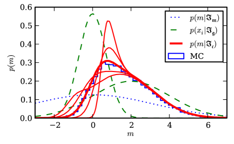
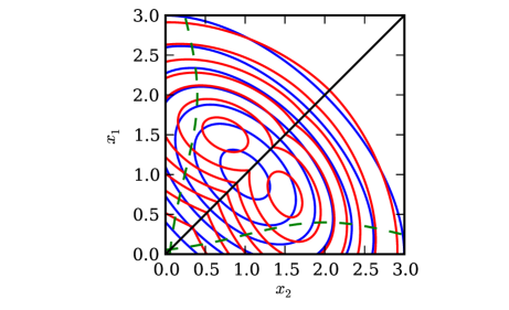
Figure 2: Illustrative plots for the analytical form of the forward and inverse posteriors. Left: Inference on $m$. Prior distribution and marginals on $\boldsymbol{x_{i}}$. Posteriors for five different values of $\rho$: -0.9 (most peaked), -0.5, 0.0 (thick line), 0.5 and 0.9 (broadest). As an experimental verification, a histogram of 20,000 samples from the posterior (generated by rejection sampling, with $\rho=0$) is shown in blue. Right: Inference on the inverse problem: Prior with $\mu_{\mathfrak{g}}=(1,1)^{\text{T}}$, $\sigma_{\mathfrak{g}1}=\sigma_{\mathfrak{g}2}=1$ and $\rho=-0.5$. Data on $m$ with $\mu_{\mathfrak{m}}=1$, $\sigma_{\mathfrak{m}}=1$ gives the posterior in red. Note the bimodality arising in this particular case.

2.4 Moment Matching

Figure 3: Factor graph representation of the functional relationships in the inference problems

The analytical forms derived in the preceeding sections are clearly not members of the normal exponential family. If $\boldsymbol{x}$ has more than two elements, they also quickly take on complicated forms that are expensive to evaluate. If the application in question allows, it might thus be desirable to find Gaussian approximations to the posteriors. This section contains derivations for the first two moments of both posteriors. The Gaussian distributions $q$ matching these moments minimize the Kullback-Leibler divergence $D_{\text{KL}}(p||q)=\int p(y)\log(p(y)/q(y))\operatorname{d}\!y$ to the correct posterior $p$ within the Gaussian family (see, e.g. Bishop, 2006, Section 10.7)).

2.4.1 Forward Problem

We will denote the mean and variance of the posterior of the max as $\mu_{m(12)}$ and $\sigma_{m(12)}^{2}$ for reasons that will become clear in Section 3. The corresponding integrals to solve are

$$\langle m\rangle \equiv\mu_{m(12)}=\int_{-\infty}^{\infty}mp(m|\mathfrak{I}_{\mathfrak{c}})\operatorname{d}\!m=Z^{-1}\int m(\nu_{1}+\nu_{2})\operatorname{d}\!m$$ (24)

$$\langle m^{2}\rangle-\langle m\rangle^{2} \equiv\sigma_{m(12)}^{2}=\int_{-\infty}^{\infty}m^{2}p(m|\mathfrak{I}_{\mathfrak{c}})\operatorname{d}\!m$$

Comparison with Equation (16) shows that these two integrals are solved by Equation (11). The solutions are thus, after some algebra,

$$\mu_{m(12)} =w_{1}\left[\mu_{\mathfrak{c}1}+\sigma_{\mathfrak{c}1}\frac{b_{1}}{a_{1}}\frac{\phi(k_{1})}{\Phi(k_{1})}\right]+w_{2}\left[\mu_{\mathfrak{c}2}+\sigma_{\mathfrak{c}2}\frac{b_{2}}{a_{2}}\frac{\phi(k_{2})}{\Phi(k_{2})}\right]$$ (25)

$$\sigma_{m(12)}^{2} =w_{1}\left\{\left[\mu_{\mathfrak{c}1}^{2}+\sigma_{\mathfrak{c}1}^{2}\right]+\left[2\mu_{\mathfrak{c}1}\sigma_{\mathfrak{c}1}\frac{b_{1}}{a_{1}}-k_{1}\sigma_{\mathfrak{c}1}^{2}\frac{b_{1}^{2}}{a_{1}^{2}}\right]\frac{\phi(k_{1})}{\Phi(k_{1})}\right\}$$

$$\qquad+w_{2}\left\{\left[\mu_{\mathfrak{c}2}^{2}+\sigma_{\mathfrak{c}2}^{2}\right]+\left[2\mu_{\mathfrak{c}2}\sigma_{\mathfrak{c}2}\frac{b_{2}}{a_{2}}-k_{2}\sigma_{\mathfrak{c}2}^{2}\frac{b_{2}^{2}}{a_{2}^{2}}\right]\frac{\phi(k_{2})}{\Phi(k_{2})}\right\}-\mu_{m(12)}^{2}$$

where

$$w_{1} =Z^{-1}\mathcal{N}(\mu_{\mathfrak{m}};\mu_{\mathfrak{g}1},\sigma_{\mathfrak{m}}^{2}+\sigma_{1}^{2})\Phi(k_{1}) w_{2} =Z^{-1}\mathcal{N}(\mu_{\mathfrak{m}};\mu_{\mathfrak{g}2},\sigma_{\mathfrak{m}}^{2}+\sigma_{2}^{2})\Phi(k_{2})$$ (26)

$$a_{1} =\left[\sigma_{\mathfrak{g}1}^{2}\sigma_{\mathfrak{g}2}^{2}(1-\rho^{2})+(\sigma_{\mathfrak{g}1}-\rho\sigma_{\mathfrak{g}2})^{2}\sigma_{\mathfrak{c}1}^{2}\right]^{1/2} a_{2} =\left[\sigma_{\mathfrak{g}1}^{2}\sigma_{\mathfrak{g}2}^{2}(1-\rho^{2})+(\sigma_{\mathfrak{g}2}-\rho\sigma_{\mathfrak{g}1})^{2}\sigma_{\mathfrak{c}2}^{2}\right]^{1/2}$$ (27)

$$b_{1} =\sigma_{\mathfrak{c}1}(\sigma_{\mathfrak{g}1}-\rho\sigma_{\mathfrak{g}2}) b_{2} =\sigma_{\mathfrak{c}2}(\sigma_{\mathfrak{g}2}-\rho\sigma_{\mathfrak{g}1})$$ (28)

2.4.2 Inverse Problem

The derivation for the inverse problem is just slightly more involved. We are interested in the moments of the marginals $p(x_{1}|\mathfrak{I}_{\mathfrak{c}})$ and $p(x_{2}|\mathfrak{I}_{\mathfrak{c}})$, and will denote these means and variances with $\mu_{1(m2)}$, $\sigma_{1(m2)}^{2}$, et cetera. From Equation (23), we get

$$\mu_{1(m2)}=\langle x_{1}\rangle_{\mathfrak{I}_{\mathfrak{c}}} =\int_{-\infty}^{\infty}x_{1}\int_{-\infty}^{x_{1}}\mathcal{N}(x_{1};\mu_{\mathfrak{m}},\sigma_{\mathfrak{m}}^{2})\mathcal{N}(\boldsymbol{x};\boldsymbol{\mu}_{\mathfrak{g}},\boldsymbol{\Sigma}_{\mathfrak{g}})\operatorname{d}\!x_{2}\operatorname{d}\!x_{1}$$ (29)

$$\quad+\int_{-\infty}^{\infty}\int_{-\infty}^{x_{2}}x_{1}\mathcal{N}(x_{2};\mu_{\mathfrak{m}},\sigma_{\mathfrak{m}}^{2})\mathcal{N}(\boldsymbol{x};\boldsymbol{\mu}_{\mathfrak{g}},\boldsymbol{\Sigma}_{\mathfrak{g}})\operatorname{d}\!x_{1}\operatorname{d}\!x_{2}$$

The first integral is in fact identical to the first term of $\mu_{m(12)}$. The second term, however, involves the first incomplete moment:

$$\int_{-\infty}^{\infty}\int_{-\infty}^{x_{2}}x_{1}\mathcal{N}(x_{2};\mu_{\mathfrak{m}},\sigma_{\mathfrak{m}}^{2})\mathcal{N}(\boldsymbol{x};\boldsymbol{\mu}_{\mathfrak{g}},\boldsymbol{\Sigma}_{\mathfrak{g}})\operatorname{d}\!x_{1}\operatorname{d}\!x_{2}$$ (30)

$$=\int_{-\infty}^{\infty}\mathcal{N}(x_{2};\mu_{\mathfrak{m}},\sigma_{\mathfrak{m}}^{2})\mathcal{N}(x_{2};\mu_{\mathfrak{g}2},\sigma_{\mathfrak{g}2}^{2})\int_{-\infty}^{x_{2}}x_{1}\mathcal{N}\left[x_{1};\mu_{\mathfrak{g}1}+\rho\frac{\sigma_{\mathfrak{g}1}}{\sigma_{\mathfrak{g}2}}(x_{2}-\mu_{\mathfrak{g}2}),\sigma^{2}_{\mathfrak{g}1}(1-\rho^{2})\right]\operatorname{d}\!x_{1}\operatorname{d}\!x_{2}$$

The inner integral can be solved using the result given in Equation (10), leading to an expression solved by Equation (11). After a bit of algebra, we arrive at the final result

$$\mu_{1(m2)} =w_{1}\left[\mu_{\mathfrak{c}1}+\sigma_{\mathfrak{c}1}\frac{b_{1}}{a_{1}}\frac{\phi(k_{1})}{\Phi(k_{1})}\right]+w_{2}\left[\left(\mu_{\mathfrak{g}1}+\rho\frac{\sigma_{\mathfrak{g}1}}{\sigma_{\mathfrak{g}2}}(\mu_{\mathfrak{c}2}-\mu_{\mathfrak{g}2})\right)+\frac{A}{a_{2}}\frac{\phi(k_{2})}{\Phi(k_{2})}\right]$$ (31)

$$\sigma^{2}_{1(m2)} =w_{1}\left\{\left[\mu_{\mathfrak{c}1}^{2}+\sigma_{\mathfrak{c}1}^{2}\right]+\left[2\mu_{\mathfrak{c}1}\sigma_{\mathfrak{c}1}\frac{b_{1}}{a_{1}}-k_{1}\sigma_{\mathfrak{c}1}^{2}\frac{b_{1}^{2}}{a_{1}^{2}}\right]\frac{\phi(k_{1})}{\Phi(k_{1})}\right\}$$

$$\qquad+w_{2}\left\{\sigma_{\mathfrak{g}1}^{2}\left[\left(\frac{\mu_{\mathfrak{g}1}}{\sigma_{\mathfrak{g}1}}+\rho\frac{(\mu_{\mathfrak{c}2}-\mu_{\mathfrak{g}2})}{\sigma_{\mathfrak{g}2}}\right)^{2}+(1-\rho^{2})+\rho^{2}\frac{\sigma_{\mathfrak{c}2}^{2}}{\sigma^{2}_{\mathfrak{g}2}}\right]\right.$$

$$\qquad\left.+\left[\frac{B}{h(1+\sigma_{\mathfrak{c}2}^{2}/h^{2})^{1/2}}-\frac{C}{h^{3}(1+\sigma_{\mathfrak{c}2}^{2}/h^{2})^{3/2}}\right]\frac{\phi(k_{2})}{\Phi(k_{2})}\right\}-\mu_{1}^{2}$$

where

$$A =\rho\sigma_{\mathfrak{c}2}^{2}\sigma_{\mathfrak{g}1}\left(1-\rho\frac{\sigma_{\mathfrak{g}1}}{\sigma_{\mathfrak{g}2}}\right)-\sigma_{\mathfrak{g}1}^{2}\sigma_{\mathfrak{g}2}(1-\rho^{2})$$ (32)

$$B =2\rho^{2}\frac{\sigma_{\mathfrak{g}1}^{2}}{\sigma_{\mathfrak{g}2}^{2}}\sigma_{\mathfrak{c}2}^{2}(\mu_{\mathfrak{c}2}-\mu_{\mathfrak{g}2})+\rho\frac{\sigma_{\mathfrak{g}1}}{\sigma_{\mathfrak{g}2}}\left(2\sigma_{\mathfrak{c}2}^{2}\mu_{\mathfrak{g}1}+\mu_{\mathfrak{g}2}\frac{\sigma_{\mathfrak{g}1}^{2}\sigma_{\mathfrak{g}2}(1-\rho^{2})}{\sigma_{\mathfrak{g}2}-\rho\sigma_{\mathfrak{g}1}}\right)-\mu_{\mathfrak{g}1}\sigma_{\mathfrak{g}1}^{2}(1-\rho^{2})\frac{\sigma_{\mathfrak{g}2}}{\sigma_{\mathfrak{g}2}-\rho\sigma_{\mathfrak{g}1}}$$

$$C =\rho^{2}\frac{\sigma_{\mathfrak{g}1}^{2}}{\sigma_{\mathfrak{g}2}^{2}}\sigma_{\mathfrak{c}2}^{4}(\mu_{\mathfrak{c}2}-f)+\sigma_{\mathfrak{g}1}^{2}(1-\rho^{2})\left(1+\rho\frac{\sigma_{\mathfrak{g}1}}{\sigma_{\mathfrak{g}2}}\right)\frac{\sigma_{\mathfrak{g}2}}{\sigma_{\mathfrak{g}2}-\rho\sigma_{\mathfrak{g}1}}(\mu_{\mathfrak{c}2}h^{2}+f\sigma_{\mathfrak{c}2}^{2})$$

with

$$f=\frac{\sigma_{\mathfrak{g}2}\mu_{\mathfrak{g}1}-\rho\sigma_{\mathfrak{g}1}\mu_{\mathfrak{g}2}}{\sigma_{\mathfrak{g}2}-\rho\sigma_{\mathfrak{g}1}}\qquad\text{and}\qquad h=\frac{\sigma_{\mathfrak{g}1}\sigma_{\mathfrak{g}2}(1-\rho^{2})^{1/2}}{\sigma_{\mathfrak{g}2}-\rho\sigma_{\mathfrak{g}1}}\\$$ (33)

The corresponding result for the posterior marginal on $x_{2}$ can be derived trivially from these results by exchanging the indices $1$ and $2$. Note that, as mentioned above, the first terms of these mixtures are shared with the posterior for $m$. Intuitively, this can be interpreted as follows: For the posterior on $m$, the first term ($\nu_{1}$) corresponds to the statement that “if $x_{1}>x_{2}$” (the probability of this is encoded by the cumulative density term in Equation (16)) “then $m$ is distributed like $x_{1}$” (represented by the product of the probability density functions in (16)). This part of the relationship features in the inverse problem as well: If $x_{1}>x_{2}$, then $x_{1}$ is distributed like $m$. The second term in the posterior marginal on $x_{1}$ corresponds to the statement that “if $x_{1}<x_{2}$, then $x_{2}$ is distributed like $m$ and $x_{1}$ is distributed such that its distribution fits with the updated marginal of $x_{2}$ given the correlation between $x_{1}$ and $x_{2}$ and the prior marginal on $x_{1}$.

2.4.3 Related Work

The moments of the likelihood of the max have been derived before by Clark (1961). That is, for $\sigma_{\mathfrak{m}}\to\infty$, the posterior $p(m|\mathfrak{I}_{\mathfrak{c}})$ reported here simplifies to a result reported by Clark:

$$\mu_{m(12)} \to\Phi(k)\left[\mu_{\mathfrak{g}1}+\sigma_{\mathfrak{g}1}\frac{(\sigma_{\mathfrak{g}1}-\rho\sigma_{\mathfrak{g}2})}{a}\frac{\phi(k)}{\Phi(k)}\right]+\Phi(-k)\left[\mu_{\mathfrak{g}2}+\sigma_{\mathfrak{g}2}\frac{(\sigma_{\mathfrak{g}2}-\rho\sigma_{\mathfrak{g}1})}{a}\frac{\phi(-k)}{\Phi(-k)}\right]$$ (34)

$$\sigma_{m(12)}^{2} \to\Phi(k)\left\{\left[\mu_{\mathfrak{g}1}^{2}+\sigma_{\mathfrak{g}1}^{2}\right]+\left[2\mu_{\mathfrak{g}1}\sigma_{\mathfrak{g}1}\frac{(\sigma_{\mathfrak{g}1}-\rho\sigma_{\mathfrak{g}2})}{a}-k\sigma_{\mathfrak{g}1}^{2}\frac{(\sigma_{\mathfrak{g}1}-\rho\sigma_{\mathfrak{g}2})^{2}}{a^{2}}\right]\frac{\phi(k)}{\Phi(k)}\right\}$$

$$\qquad+\Phi(-k)\left\{\left[\mu_{\mathfrak{g}2}^{2}+\sigma_{\mathfrak{g}2}^{2}\right]+\left[2\mu_{\mathfrak{g}2}\sigma_{\mathfrak{g}2}\frac{(\sigma_{\mathfrak{g}2}-\rho\sigma_{\mathfrak{g}1})}{a}+k\sigma_{\mathfrak{g}2}^{2}\frac{(\sigma_{\mathfrak{g}2}-\rho\sigma_{\mathfrak{g}1})^{2}}{a^{2}}\right]\frac{\phi(-k)}{\Phi(-k)}\right\}$$

$$\qquad-\mu_{m(12)}^{2}$$

$$\text{where}\quad a =\sqrt{\sigma^{2}_{\mathfrak{g}1}+\sigma^{2}_{\mathfrak{g}2}-2\rho\sigma_{\mathfrak{g}1}\sigma_{\mathfrak{g}2}}\qquad\text{and}\qquad k=\frac{\mu_{\mathfrak{g}1}-\mu_{\mathfrak{g}2}}{a}$$

As expected, the posterior of the inverse problem simply becomes equal to the prior in this case. From Equation (31) we find

$$\mu_{1(m2)} \to\Phi(k)\mu_{1}+\sigma_{1}\frac{\sigma_{1}-\rho\sigma_{2}}{a}\phi(k)+\Phi(-k)\mu_{1}-\sigma_{1}\frac{\sigma_{1}-\rho\sigma_{2}}{a}\phi(-k)$$ (35)

$$=\Phi(k)\mu_{1}+\sigma_{1}\frac{\sigma_{1}-\rho\sigma_{2}}{a}\phi(k)+(1-\Phi(k))\mu_{1}-\sigma_{1}\frac{\sigma_{1}-\rho\sigma_{2}}{a}\phi(k)$$

$$=\mu_{1}$$

and similarly for the variance.

The max-factor is also part of the Infer.net software package (Minka and Winn, 2008) (to my knowledge, the derivations for this code have not been published yet). However, their implementation can only handle two independent Gaussian inputs (Section 3 introduces the max over a finite set of correlated variables). So their implementation corresponds to the case of $\rho=0$, which leads to the following simplifications, presented here for reference:

$$k_{1} =\frac{\mu_{\mathfrak{c}1}-\mu_{\mathfrak{g}2}}{(\sigma_{\mathfrak{g}1}+\sigma_{\mathfrak{c}2})^{1/2}} a_{1} =\sigma_{\mathfrak{g}1}(\sigma_{\mathfrak{g}1}+\sigma_{\mathfrak{c}2})^{1/2} b_{1} =\sigma_{\mathfrak{c}1}\sigma_{\mathfrak{g}1}$$ (36)

$$A =\sigma_{\mathfrak{g}1}^{2}\sigma_{\mathfrak{g}2} B =-\mu_{\mathfrak{g}1}\sigma_{\mathfrak{g}1}^{2} C =\sigma_{\mathfrak{g}1}^{2}(\mu_{\mathfrak{c}2}\sigma_{\mathfrak{g}1}^{2}+\mu_{\mathfrak{g}1}\sigma_{\mathfrak{c}2}^{2})$$ (37)

$$f =\mu_{\mathfrak{g}1} h =\sigma_{\mathfrak{g}1}$$ (38)

Figure 4 shows some of these approximations. The parameter settings used in this figure represent a worst case (e.g., the posterior over $\boldsymbol{x}$ is rarely so strongly bimodal.)

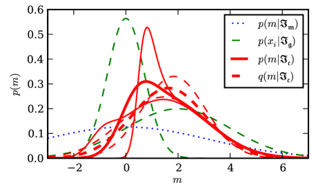
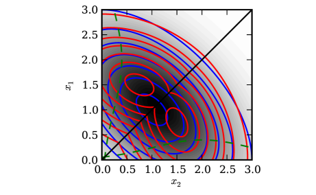
Figure 4: Illustrative plots for the Gaussian approximations to the posteriors. Same beliefs in $\mathfrak{I}_{\mathfrak{c}}$ as in Figure 2. Left: For the sake of readability, only the cases $\rho=-0.9$ (broadest), $\rho=0$ and $\rho=0.9$ are plotted here. In red, dashed lines the corresponding three Gaussian approximations. Note the varying quality of fit. Right: Gaussian approximation (with $\boldsymbol{\mu}_{1(m2)}=1.06$ and $\sigma_{1(m2)}^{2}=0.94$) indicated by shaded area.

3 The Maximum of a Finite Set

Figure 5: Factor graph representation of the inference problem on a finite set. The dashed “plate” represents $N$ copies of generating variable nodes.

3.1 Analytic Form

Extending the analysis of Section 2.3, we can write the posterior over the max $m$ of a finite set $\{x_{i}\}_{i=1,\dots,N}$ of variables, distributed according to an $N$-dimensional version of Equation (1), with a new normalization constant $Z_{N}$, as

$$p(m|\mathfrak{I}_{\mathfrak{c}}) =Z_{N}p(m|\mathfrak{I}_{\mathfrak{m}})\int p(\boldsymbol{x}|m)p(\boldsymbol{x}|\mathfrak{I}_{\mathfrak{g}})\operatorname{d}\!\boldsymbol{x}$$ (39)

$$=Z_{N}\mathcal{N}(m;\mu_{\mathfrak{m}},\sigma_{\mathfrak{m}})\left[\sum_{i=1}^{N}\int_{-\infty}^{\infty}\delta(m-x_{i})p(x_{i}|\mathfrak{I}_{\mathfrak{g}})\idotsint_{-\infty}^{x_{i}}p(\{x_{j}\}_{j\neq i}|x_{i},\mathfrak{I}_{\mathfrak{g}})\prod_{j\neq i}\operatorname{d}\!x_{j}\operatorname{d}\!x_{i}\right]$$

$$=Z_{N}\sum_{i}\left[\mathcal{N}(\mu_{\mathfrak{m}};\mu_{\mathfrak{g}i},\sigma_{\mathfrak{m}}^{2}+\sigma_{\mathfrak{g}i}^{2})\mathcal{N}(m;\mu_{\mathfrak{c}i},\sigma_{\mathfrak{c}i}^{2})\idotsint_{-\infty}^{x_{i}}\mathcal{N}(\boldsymbol{x}_{\setminus i};\boldsymbol{\mu}_{\mathfrak{g}\setminus i}(x_{i}),\boldsymbol{\Sigma}_{\mathfrak{g}\setminus i})\operatorname{d}\!\boldsymbol{x}_{\setminus i}\right]$$

where $\boldsymbol{x}_{\setminus i}=(x_{1},\dots,x_{i-1},x_{i+1},\dots,x_{N})$. The conditional mean is (see e.g. Bishop, 2006, Section 2.3.2)

$$\left(\boldsymbol{\mu}_{\setminus i}(x_{i})\right)_{j}=\mu_{\mathfrak{g}j}+\Sigma_{\mathfrak{g}ji}\Sigma_{\mathfrak{g}ii}^{-1}(x_{i}-\mu_{\mathfrak{g}i})=\mu_{\mathfrak{g}j}+\rho_{ij}\frac{\sigma_{\mathfrak{g}j}}{\sigma_{\mathfrak{g}i}}(x_{i}-\mu_{\mathfrak{g}i})$$ (40)

with the linear coefficient of correlation $\rho_{ij}=\Sigma_{\mathfrak{g}ij}/(\sigma_{\mathfrak{g}i}\sigma_{\mathfrak{g}j})$. The conditional covariance matrix is the Schur complement of $\Sigma_{\mathfrak{g}ii}=\sigma_{\mathfrak{g}i}^{2}$ in $\boldsymbol{\Sigma_{\mathfrak{g}}}$:

$$\Sigma_{\mathfrak{g}\setminus i,kj}=\Sigma_{\mathfrak{g}kj}-\Sigma_{\mathfrak{g}ki}\sigma_{\mathfrak{g}i}^{-2}\Sigma_{\mathfrak{g}ij}$$ (41)

In principle, it would be possible to follow the path laid out in the previous sections to calculate the first two moments of this distribution. However, while the univariate Gaussian CDF (essentially an evaluation of the error function) has computational cost comparable to evaluating an exponential function, computationally efficient ways of calculating a multivariate Gaussian CDF are not generally available. So this approximation would need to involve an undesirable numerical integration.

3.2 A Heuristic Approximation

Another, cheaper option is to use an iterative procedure initially proposed by Clark (1961). The idea is to start out with the approximation for only two of the generating variables. W.l.o.g., let these be $x_{1}$ and $x_{2}$, resulting in $m_{(12)}=\max(x_{1},x_{2})$. Next, estimate $m_{(123)}=\max(x_{3},m_{(12)})$ and so on up to $m_{(1\dots N)}$. For the intermediate maxima, the likelihoods presented in Equation (34) suffice, and the prior is included in the last step (using Equation (25)) to gain an approximate posterior over the maximum of the whole set. Of course, this necessitates an analytic expression for the correlation coefficient $\rho_{i(1\dots i-1)}$ between the $i$-th variable and the max over the preceding variables. This was derived by Clark. Adopted to the notation used here and made more explicit, his result is

$$\rho_{3(12)}=\sigma_{(12)}^{-1}\left(\sigma_{1}\rho_{31}\Phi(k_{(12)})+\sigma_{2}\rho_{32}\Phi(-k_{(12)})\right)$$ (42)

where $\rho_{ij}=\Sigma_{ij}/\sigma_{i}\sigma_{j}$, the index $\mathfrak{g}$ has been dropped for simplicity and $k_{(12)}=(\mu_{1}-\mu_{2})/\sqrt{\sigma_{1}^{2}+\sigma_{2}^{2}}$ is the simplified version of $k_{1}$ arising from Equation (20) under $\sigma_{\mathfrak{m}}\to\infty$. Using this, we can build a recursive algorithm to calculate $\rho_{i(1\dots j)}$ with $j<i$ as

$$\rho_{i(1\dots j)}=\sigma_{(1\dots j)}^{-1}\cdot\begin{cases}\sigma_{j}\rho_{ij}&\text{if~{}}j=1\\ \Phi(-k_{(1\dots j)})\sigma_{j}\rho_{ij}+\Phi(k_{(1\dots j)})\rho_{i(1\dots j-1)}&\text{else}\end{cases}$$ (43)

this necessitates a list $\boldsymbol{k}_{[j]}=(k_{(12)},\dots k_{(1\dots i-1)})$ which is available at the necessary point in time from the calculation of previous maxima over the preceding parts of the set. Note that calculating $\rho_{i(1\dots i-1)}$ involves $i-1$ recursive function calls, so building the full approximation over the max of $N$ variables is of complexity $\mathcal{O}(N^{2})$, as might be expected (although there are only $(N-1)$ uses of the results in Equation (25)). If all correlation coefficients are the same, $\rho_{ij}=\rho\>\forall ij$, then the recursive evaluations can be re-used in consecutive evaluations and the complexity drops to $\mathcal{O}(N)$.

3.2.1 Inverse Problem

The same iterative scheme can be used to provide an approximation for the inverse problem’s posterior. First, the list $\boldsymbol{k}_{[j]}$ is build as in the preceding section. Then, approximations to the posterior marginals are build iteratively, starting with $q(x_{N}|\mathfrak{I}_{\mathfrak{c}})$, ending with $q(x_{2}|\mathfrak{I}_{\mathfrak{c}})$ and $q(x_{1}|\mathfrak{I}_{\mathfrak{c}})$. At each intermediate step, we use the EP approximation (Minka, 2001): To get $q(x_{i}|\mathfrak{I}_{\mathfrak{c}})$, use $q(m_{(1\dots i)}|\mathfrak{I}_{\mathfrak{m}})=q(m_{(1\dots i)}|\mathfrak{I}_{\mathfrak{c}})/q(m_{(1\dots i)}|\mathfrak{I}_{\mathfrak{g}})$ as an approximation to the prior over the subset max, and $q(m_{(1\dots i-1)}|\mathfrak{I}_{\mathfrak{g}})$ as the approximation on the max over the subset up to $x_{i-1}$.

4 Discussion of the Approximation’s Quality

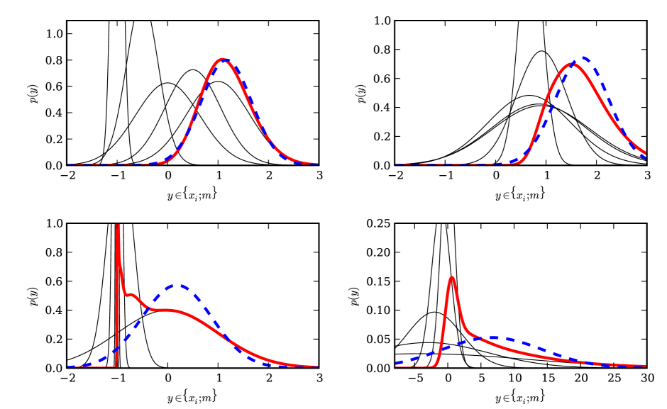
Figure 6: Quality and failure modes of the EP approximation. Max of five uncorrelated Gaussians. Top row: examples of good fits. Left: well separated beliefs. Right: similar beliefs. Bottom row: worst case examples. Left: high certainty contributions within the center. Right: high uncertainty in one tail. In all plots, beliefs over the $x_{i}$ as slim black lines. True posterior over $m$ in thick red, approximation in thick dashed blue. For simplicity, $p(m|\mathfrak{I}_{\mathfrak{m}})$ was set to an uninformative value. See text for details.

Figure 6 gives some intuition on the quality of the approximation. For the purpose of this comparison, uncorrelated Gaussians were used because this allows the analytic evaluation of the true posterior (the CDF factorises into individual one-dimensional CDFs). The fit is reasonably good if the beliefs over the $x_{i}$ are either very similar (Figure 6 top right), or if the beliefs are “separated”, in the sense that one of the $x_{i}$ provides a dominant contribution to the overall mixture (top left). The fit becomes bad when the mixture has many modes (bottom left) or a strong asymmetry (bottom right). The corresponding worst case distributions shown here were generated by setting $\mu_{\mathfrak{g}i}=a+b^{-i}$ and $\sigma_{\mathfrak{g}i}^{2}=b^{-i}$ (left, $a=-1,b=16$) or $\mu_{\mathfrak{g}i}=ci$ and $\sigma_{\mathfrak{g}i}^{2}=i^{d}+1$ (right, $c=-1,d=16$). More quantitatively, consider Equation (34) or Equation (16), the case of the max of only two Gaussians. The two cases of good fit described above correspond to

1. one mixture component dominating the mixture

   $$|k_{12}|=\frac{|\mu_{\mathfrak{g}1}-\mu_{\mathfrak{g}2}|}{\sqrt{\sigma_{\mathfrak{g}1}^{2}+\sigma_{\mathfrak{g}2}^{2}-2\rho\sigma_{\mathfrak{g}1}\sigma_{\mathfrak{g}2}}}\gg 0$$ (44)

   The likelihood then has one clearly dominating Gaussian component and the fit is good. In this case, the inverse problem is also a good fit, as each of the generating variables $x_{1},x_{2}$ has one dominating component in its posterior.

2. the two mixture components being almost identical:

   $$\mu_{\mathfrak{g}1}\approx\mu_{\mathfrak{g}2}\qquad\text{and}\qquad\sigma_{\mathfrak{g}1}\approx\sigma_{\mathfrak{g}2}$$ (45)

   the likelihood then consists of two roughly identical Gaussian components with roughly the same weights, and is therefore roughly Gaussian. However, the approximation is bad for the inverse problem here, as the true posterior marginals become bimodal (c.f. Figure 2, right). This effect is particularly pronounced if the mean of the prior and the likelihood differ significantly.

These observations suggest a potential increase in the quality of the approximation to be gained from calculating all $N(N-1)$ weight-generators $k_{ij}$ as defined in Equation (44) and iteratively choosing the pair $ij$ with maximal $k_{ij}$. However, this re-ordering has to be updated after each incremental two-component max operation, involving a re-calculation of up to $N$ correlation coefficients. It thus raises the complexity of calculating the approximation for the overall max from $\mathcal{O}(N^{2})$ to $\mathcal{O}(N^{3})$. Initial experiments suggest that the potential gain in fit is almost always negligible.

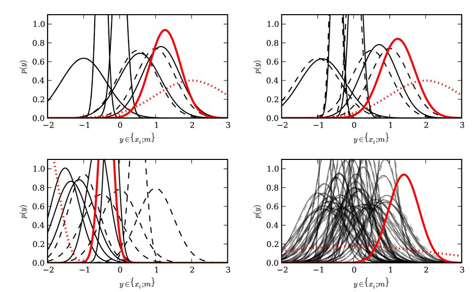
Figure 7: Illustrative examples for the use of the approximation in EP message passing. $p(x_{i}|\mathfrak{I}_{\mathfrak{g}})$ in black dashed lines. $p(m|\mathfrak{I}_{\mathfrak{m}})$ in red dotted. Marginals after EP message passing as corresponding solid lines. Top left: Max over 5 uncorrelated variables. Only the two variables contributing significantly to the max change their beliefs. Top right: same as previous, but with $\rho_{ij}=0.9$ for all $ij$. The change in belief over the dominating $x_{i}$ now also effects the other beliefs, as expected. Bottom left: The approximation is well-behaved under inconsistent beliefs. $p(m|\mathfrak{I}_{\mathfrak{m}})$ was set inconsistently low relative to the beliefs on the $x_{i}$ (all $\rho_{ij}=0.2$). Note that the belief over the largest $x_{i}$ extends beyond the belief over $m$ as a result of the moment-matching. Bottom right: The approximation is stable for large values of $N$. Maximum over 50 correlated normals, all $\rho_{ij}$ were set to 0.5.

5 Conclusion

This technical report derived the first two moments of the posterior over the maximum of a pair of Gaussian variables, and over the posterior over the two generating variables. These moments can be used for approximate Inference on their own, or as part of a larger graphical model using Expectation Propagation. I have also shown how to extend the usefulness of these approximations to finite sets of Gaussian variables using a heuristic iterative approximation. The quality of the approximation depends on the location and precision of the belief over the generating variables relative to each other, but is always good enough to provide a meaningful point estimate and error measure. It is sufficiently robust to deal with inconsistent belief assignments and large numbers of generating variables (see Figure 7).

References

- Ahuja and Orlin [2001] R.K. Ahuja and J.B. Orlin. Inverse optimization. Operations Research, pages 771–783, 2001.
- Bishop [2006] C.M. Bishop. Pattern recognition and machine learning. Springer New York., 2006.
- Burton and Toint [1992] D. Burton and P.L. Toint. On an instance of the inverse shortest paths problem. Mathematical Programming, 53(1):45–61, 1992.
- Clark [1961] Charles E. Clark. The greatest of a finite set of random variables. Operations Research, 9(2):145–162, 1961.
- Dearden et al. [1998] Richard Dearden, Nir Friedman, and Stuart Russell. Bayesian Q-learning. In In AAAI/IAAI, pages 761–768. AAAI Press, 1998.
- Heuberger [2004] C. Heuberger. Inverse combinatorial optimization: A survey on problems, methods, and results. Journal of Combinatorial Optimization, 8(3):329–361, 2004.
- Minka and Winn [2008] Thomas Minka and John Winn. infer.NET software package. Microsoft Research Ltd., 2008.
- Minka [2001] T.P. Minka. Expectation Propagation for approximate Bayesian inference. In Proceedings of the 17th Conference in Uncertainty in Artificial Intelligence table of contents, pages 362–369. Morgan Kaufmann Publishers Inc. San Francisco, CA, USA, 2001.
- Neumann-Denzau and Behrens [1984] G. Neumann-Denzau and J. Behrens. Inversion of seismic data using tomographical reconstruction techniques for investigations of laterally inhomogeneous media. Geophysical Journal International, 79(1):305–315, 1984.
- Rasmussen and Williams [2006] Carl Edward Rasmussen and Christopher K. I. Williams. Gaussian Processes for Machine Learning. MIT Press, 2006.