Random walk in two-dimensional self-affine random potentials :
strong disorder renormalization approach

Abstract

We consider the continuous-time random walk of a particle in a two-dimensional self-affine quenched random potential of Hurst exponent $H>0$. The corresponding master equation is studied via the strong disorder renormalization procedure introduced in Ref. [C. Monthus and T. Garel, J. Phys. A: Math. Theor. 41 (2008) 255002]. We present numerical results on the statistics of the equilibrium time $t_{eq}$ over the disordered samples of a given size $L\times L$ for $10\leq L\leq 80$. We find an ’Infinite disorder fixed point’, where the equilibrium barrier $\Gamma_{eq}\equiv\ln t_{eq}$ scales as $\Gamma_{eq}=L^{H}u$ where $u$ is a random variable of order $O(1)$. This corresponds to a logarithmically-slow diffusion $|\vec{r}(t)-\vec{r}(0)|\sim(\ln t)^{1/H}$ for the position $\vec{r}(t)$ of the particle.

I Introduction

Random walks and diffusion processes have been the subject of constant interest in mathematics and in physics during the last century, for two main reasons (i) they play a central role in probability theory, and present a large number of very nice mathematical properties (ii) they naturally appear in a great variety of situations in physics and in biology. It is thus important to understand the effects of quenched disorder on random walks : are the usual properties of random walks stable with respect to the presence of some disorder or inhomogeneity ? If not, what are the new properties induced by disorder? Among the various types of random walks in random media that have been considered in the past (see the reviews [1, 2, 3] and references therein), we wish to focus here on the case of random walks in a two-dimensional self-affine random potential $U(\vec{r})$. In a continuous framework, this model can be defined via the Langevin equation for the position $\vec{r}$ of the particle

$$\frac{d\vec{r}}{dt}=-\vec{\nabla}U(\vec{r})+\vec{\eta}(t)$$ (1)

where $\vec{\eta}(t)$ is a white noise

$$<\eta_{i}(t)\eta_{j}(t^{\prime})>=2T\delta(t-t^{\prime})\delta_{i,j}$$ (2)

that would generate a Brownian diffusion in the absence of the random potential $U$, and where the quenched random potential $U(\vec{r})$ is self-affine with some Hurst exponent $H$

$$\overline{\left[U(\vec{r})-U(\vec{r}\ ^{\prime})\right]^{2}}\mathop{\simeq}_{|\vec{r}-\vec{r}\ ^{\prime}|\to\infty}|\vec{r}-\vec{r}\ ^{\prime}|^{2H}$$ (3)

The case of dimension $d=1$ and Hurst exponent $H=1/2$ corresponds to the random-force Sinai model where the logarithmically-slow behavior $|r(t)-r(0)|\sim(\ln t)^{2}$ has been obtained via various exact methods (see for instance the review [3] and references therein). Since this logarithmic behavior replaces the usual power-law behaviour $x\sim\sqrt{t}$ of the pure Brownian motion, the effect of disorder is extremely strong. In higher dimension $d>1$, the model is not exactly solvable, but from scaling arguments on barriers, one still expects the analogous logarithmic scaling [4, 3]

$$|\vec{r}(t)-\vec{r}(0)|\sim(\ln t)^{1/H}$$ (4)

However, to the best of our knowledge, this behavior has not been much tested, except in the preliminary unpublished numerical results of Pettini shown on Fig. 4.9 of the review [3]. The aim of this paper is to study a continuous-time lattice version of this model in dimension $d=2$, via the strong disorder renormalization procedure introduced in [5] that can be applied to any master equation in arbitrary dimension.

The paper is organized as follows. In section II, we recall the Weierstrass-Mandelbrot function method to generate numerically two-dimensional self-affine random potentials. In section III, we explain how to use for the present case the strong disorder renormalization method introduced in [5]. In section IV, we present our numerical results concerning the statistics of the equilibrium time $t_{eq}$ over the disordered samples of a given size $L\times L$. Our conclusions are summarized in section V.

II Method for generating a two-dimensional self-affine random potential

Among the various methods that have been proposed in the literature to generate random functions of a given Hurst exponent (see the reviews [6] and a comparative study of their performances in [7]), we have found numerically that the method giving the best results for the correlation of Eq. 3 is the so-called Weierstrass-Mandelbrot function method, that we recall in this section.

Figure 1: Random self-affine random potential $U(x,y)$ on a square of size $100\times 100$, obtained via the method of Eq. 6 for the value $H=0.5$ of the Hurst exponent : (a) Example of one realization of the random potential $U(x,y)$ . (b) Log-log plot of the correlation function $C(r)\equiv\overline{\left[U(\vec{r}_{1})-U(\vec{r}_{2})\right]^{2}}$ as a function of the distance $r\equiv|\vec{r}_{1}-\vec{r}_{2}|$ after averaging over angles and over disorder realizations : the slope is here $2H=1$, as it should for $H=0.5$ (see Eq. 3).

II.1 Reminder on the Weierstrass-Mandelbrot function in dimension $d=1$

In dimension $d=1$, the Weierstrass-Mandelbrot function is defined by [8, 9]

$$U(x)=\sum_{n=n_{min}}^{n_{max}}\frac{\cos(2\pi\phi_{n})-\cos\left(2\pi\gamma^{n}x+2\pi\phi_{n}\right)}{\gamma^{nH}}$$ (5)

where the phases $\phi_{n}$ are independent and uniform in $[0,1]$, and where $n_{min}=-\infty$ and $n_{max}=+\infty$. The function $U(x)$ is fractal with Hurst exponent $H$ on all scales : the frequencies $\gamma^{n}$ are in geometric progression, in contrast with a Fourier transform that would correspond to an arithmetic progression. In the limit $\gamma\to 1$, the discrete spectrum become dense and the function $U(x)$ converge towards the fractional Brownian motion of exponent $H$. We refer to [9] for more details on its mathematical properties and now discuss how to use it for numerical simulations.

If one wishes to generate the potential $U(x)$ at $N$ discrete points $x=1,2,...N$, one has to choose the three parameters $(n_{min},n_{max},\gamma)$ in the following way :

(i) the maximal Fourier frequency $\omega_{max}$ associated to the lattice spacing $\Delta x=1$ is $\omega_{max}=1/(\Delta x)=1$. A convenient choice is thus $n_{max}=0$, corresponding to the maximal frequency $\gamma^{n_{max}}=1$ in the sum of Eq. 5.

(ii) the minimal Fourier frequency $\omega_{min}$ associated to the sample size $N$ is $\omega_{min}=1/N$. Since we do not wish any periodicity of order $N$ in the potential, we have to choose $n_{min}$ such that the minimal frequency $\gamma^{n_{min}}$ in the sum of Eq. 5 satisfies $\gamma^{n_{min}}\ll 1/N$.

(iii) finally, the parameter $\gamma$ determines the discretization of the frequency spectrum : the frequency $\gamma^{n}$ have to be sufficiently dense.

We now turn to the generalization to higher dimension.

II.2 Generalization to dimension $d=2$

To generalise Eq. 5 to higher dimension $d>1$, the idea [10, 11] is to keep the principle of a sum over plane waves of various vectors $\vec{k}$, where the modulus $|\vec{k}|$ varies in geometric progression $\gamma^{n}$, and where the angular part of $\vec{k}$ is uniformly distributed to insure isotropy. In dimension $d=2$, this corresponds to [10, 11]

$$U(x,y)=\sum_{n=n_{min}}^{n_{max}}\frac{1}{\sqrt{m}_{max}}\sum_{m=1}^{m_{max}}\frac{\cos(2\pi\phi_{n,m})-\cos\left(2\pi\gamma^{n}(x\cos 2\pi\alpha_{n,m}+y\sin 2\pi\alpha_{n,m})+2\pi\phi_{n,m}\right)}{\gamma^{nH}}$$ (6)

where the phases $\alpha_{n,m}$ and $\phi_{n,m}$ are independent and uniformly distributed in $[0,1]$. The new parameter $m_{max}$ fixes the number of wave vectors $\vec{k}$ of a given modulus $|\vec{k}|$. We have checked that this generalization proposed in [10, 11] gives satisfactory numerical realizations of self-affine random potential (whereas the alternative generalization proposed in [12, 13] that are based on cartesian coordinates presents anisotropy).

Here we wish to generate the potential $U(x,y)$ at $N^{2}$ discrete points where $x=1,2,...N$ and $y=1,2,..,N$. One has then to choose the four parameters $(n_{min},n_{max},m_{max},\gamma)$ to obtain good results for the two-point function of Eq. 3 for all pairs of points of the samples. For squares samples of linear size $10\leq L\leq 80$, we have found that the following set of parameters give satisfactory realizations of the potential $U(x,y)$ for Hurst exponents $0.3\leq H\leq 0.8$ : $n_{max}=0$, $n_{min}=-150$, $m_{max}=100$, $\gamma=1.2$. We show on Fig. 1 (a) an example of realization of the random self-affine random potential $U(x,y)$ on a square of size $100\times 100$, for the value $H=0.5$ of the Hurst exponent. The corresponding correlation function is shown on Fig. 1 (b) on a log-log plot.

III Strong disorder renormalization procedure

Strong disorder renormalization (see [14] for a review) is a very specific type of RG that has been first developed in the field of quantum spins : the RG rules of Ma and Dasgupta [15] have been put on a firm ground by D.S. Fisher who introduced the crucial idea of “infinite disorder” fixed point where the method becomes asymptotically exact, and who computed explicitly exact critical exponents and scaling functions for one-dimensional disordered quantum spin chains [16]. This method has thus generated a lot of activity for various disordered quantum models [14], and has been then successfully applied to various classical disordered dynamical models, such as random walks in random media [17, 18], reaction-diffusion in a random medium [19], coarsening dynamics of classical spin chains [20], trap models [21], random vibrational networks [22], absorbing state phase transitions [23], zero range processes [24] and exclusion processes [25].

For random walks in random media, the procedure introduced in Refs [17, 18] or in the recent work [26] are specific to the dimension $d=1$. Here in dimension $d=2$, the appropriate framework is the ’strong disorder renormalization’ (RG) procedure introduced [5] that can be defined for any master equation. In this section, we recall its principles for the present problem of a particle in a two-dimensional potential.

III.1 Master Equation

The master equation describing the evolution of the probability $P_{t}({\vec{r}})$ to be at position ${\vec{r}}$ at time t can be written as

$$\frac{dP_{t}\left({\vec{r}}\right)}{dt}=\sum_{\vec{r}\ ^{\prime}}P_{t}\left({\vec{r}}\ ^{\prime}\right)W\left({\vec{r}}\ ^{\prime}\to{\vec{r}}\right)-P_{t}\left({\vec{r}}\right)W_{out}\left({\vec{r}}\right)$$ (7)

where $W\left({\vec{r}}\ ^{\prime}\to{\vec{r}}\right)$ represents the transition rate per unit time from position ${\vec{r}}\ ^{\prime}$ to ${\vec{r}}$, and

$$W_{out}\left({\vec{r}}\right)\equiv\sum_{{\vec{r}}^{\prime}}W\left({\vec{r}}\to{\vec{r}}\ ^{\prime}\right)$$ (8)

represents the total exit rate out of position ${\vec{r}}$.

For the two-dimensional random walk in the random potential $U(\vec{r})$ at temperature $T$, we have chosen to consider the Metropolis dynamics defined by the transition rates

$$W\left(\vec{r}\to\vec{r}\ ^{\prime}\right)=\delta_{<\vec{r},\vec{r}\ ^{\prime}>}\ {\rm min}\left(1,e^{-(U(\vec{r}\ ^{\prime})-U(\vec{r}))/T}\right)$$ (9)

The first factor $\delta_{<\vec{r},\vec{r}\ ^{\prime}>}$ means that the two positions are neighbors on the two-dimensional lattice, and the last factor ensures the convergence towards thermal equilibrium at temperature $T$ via the detailed balance property

$$e^{-U(\vec{r})/T}W\left(\vec{r}\to\vec{r}\ ^{\prime}\right)=e^{-U(\vec{r}\ ^{\prime})/T}W\left(\vec{r}\ ^{\prime}\to\vec{r}\right)$$ (10)

III.2 Strong disorder renormalization rules

For dynamical models, the aim of any renormalization procedure is to integrate over ’fast’ processes to obtain effective properties of ’slow’ processes. The general idea of ’strong renormalization’ for dynamical models consists in eliminating iteratively the ’fastest’ process. The RG procedure introduced in [5] can be summarized as follows :

(1) find the position $\vec{r}^{*}$ with the largest exit rate $W^{*}_{out}$

$$W^{*}_{out}=W_{out}\left(\vec{r}^{*}\right)\equiv{\rm max}_{\vec{r}}\left[W_{out}\left(\vec{r}\right)\right]$$ (11)

(2) find the neighbors $(\vec{r}_{1},\vec{r}_{2},...,\vec{r}_{n})$ of position $\vec{r}^{*}$, i.e. the surviving positions that are related via positive rates $W(\vec{r}^{*}\to\vec{r}_{i})>0$ and $W(\vec{r}_{i}\to\vec{r}^{*})>0$ to the decimated position $\vec{r}^{*}$. For each neighbor position $\vec{r}_{i}$ with $i\in(1,..,n)$, update the transition rate to go to the position $\vec{r}_{j}$ with $j\in(1,..,n)$ and $j\neq i$ according to

$$W^{new}(\vec{r}_{i}\to\vec{r}_{j})=W(\vec{r}_{i}\to\vec{r}_{j})+W(\vec{r}_{i}\to\vec{r}^{*})\times\pi_{\vec{r}^{*}}\left(\vec{r}_{j}\right)$$ (12)

where the first term represents the ’old’ transition rate (possibly zero), and the second term represents the transition via the decimated position $\vec{r}^{*}$ : the factor $W(\vec{r}_{i}\to\vec{r}^{*})$ takes into account the transition rate to $\vec{r}^{*}$ and the term

$$\pi_{\vec{r}^{*}}\left(\vec{r}_{j}\right)=\frac{W\left(\vec{r}^{*}\to\vec{r}_{j}\right)}{W_{out}\left(\vec{r}^{*}\right)}$$ (13)

represents the probability to make a transition towards $\vec{r}_{j}$ when in $\vec{r}^{*}$. The $2n$ rates $W(\vec{r}^{*}\to\vec{r}_{i})$ and $W(\vec{r}_{i}\to\vec{r}^{*})$ then disappear with the decimated position $\vec{r}^{*}$. Note that the rule of Eq. 12 has been recently proposed in [27] to eliminate ’fast states’ from various dynamical problems with two very separated time scales. The physical interpretation of this rule is as follows : the time spent in the decimated position $\vec{r}^{*}$ is neglected with respects to the other time scales remaining in the system. The validity of this approximation within the present renormalization procedure is discussed in detail in [5].

(3) update the exit rates out of the neighbors $\vec{r}_{i}$ of $\vec{r}^{*}$, with $i=1,..,n$ either with the definition

$$W^{new}_{out}(\vec{r}_{i})=\sum_{\vec{r}}W^{new}(\vec{r}_{i}\to\vec{r})$$ (14)

or with the rule that can be deduced from Eq. 12

$$W^{new}_{out}(\vec{r}_{i})=W_{out}(\vec{r}_{i})-W(\vec{r}_{i}\to\vec{r}^{*})\frac{W(\vec{r}^{*}\to\vec{r}_{i})}{W^{*}_{out}}$$ (15)

The physical meaning of this rule is the following. The exit rate out of the position $\vec{r}_{i}$ decays because the previous transition towards $\vec{r}^{*}$ can lead to an immediate return towards $\vec{r}_{i}$. After the decimation of the position $\vec{r}^{*}$, this process is not considered as an ’exit’ process anymore, but as a residence process in the position $\vec{r}_{i}$. This point is very important to understand the meaning of the renormalization procedure : the remaining positions at a given renormalization scale are ’formally’ microscopic positions of the initial master equation (Eq. 7), but each of these remaining microscopic position actually represents some ’valley’ in position space that takes into account all the previously decimated positions.

(4) return to point (1).

We refer to [5] for more detailed explanations. In practice, the renormalized rates $W(\vec{r}\to\vec{r}\ ^{\prime})$ can rapidly become very small as a consequence of the multiplicative structure of the renormalization rule of Eq 12. This means that the appropriate variables are the logarithms of the transition rates, that we will call ’barriers’ in the remaining of this paper. The barrier $B(\vec{r}\to\vec{r}\ ^{\prime})$ from $\vec{r}$ to $\vec{r}\ ^{\prime}$ is defined by

$$B(\vec{r}\to\vec{r}\ ^{\prime})\equiv-\ln W(\vec{r}\to\vec{r}\ ^{\prime})$$ (16)

and similarly the exit barrier out of position $\vec{r}$ is defined by

$$B_{out}(\vec{r})\equiv-\ln W_{out}(\vec{r})$$ (17)

A very important advantage of this formulation in terms of the renormalized transition rates of the master equation is that the renormalized barriers take into account the true ’barriers’ of the dynamics, whatever their origin which can be either energetic or entropic.

III.3 Numerical details

We have applied numerically these renormalization rules for square samples of size $L^{2}$ with $10\leq L\leq 80$ with a statistics of $33.10^{5}\geq n_{s}(L)\geq 280$ disordered samples. We have studied six values of the Hurst exponent in the interval $0.3\leq H\leq 0.8$.

IV Statistics of the equilibrium time of finite systems

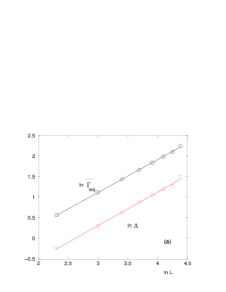
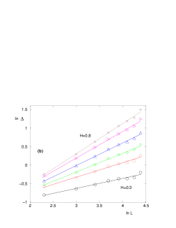
Figure 2: (Color on line) Statistics of the equilibrium time $t_{eq}$ over the disordered samples of sizes $L^{2}$ : the appropriate variable is $\Gamma_{eq}=\ln t_{eq}$ (Eq. 19) (a) the disorder-averaged value $\overline{\Gamma_{eq}}(L)$ and the width $\Delta(L)$ shown here for $H=0.8$ scale with the same exponent $\psi$ (see Eq. 20). (b) the exponent $\psi$ of the width $\Delta(L)$ coincides with the Hurst exponent $H$, as shown here for $H=0.3,0.4,0.5,0.6,0.7,0.8$

In a finite system, the master equation of Eq. 7 satisfying the detailed balance condition of Eq. 10 will converge exponentially towards the equilibrium Boltzmann distribution. The characteristic time of this exponential convergence is called the equilibrium time $t_{eq}$

$$P_{t}\left({\vec{r}}\right)-P_{eq}({\vec{r}})\mathop{\propto}_{t\to\infty}e^{-\frac{t}{t_{eq}}}$$ (18)

Within the strong disorder renormalization procedure described in the previous section, this equilibrium time $t_{eq}$ of a given disordered sample is determined by the renormalized exit barrier

$$\Gamma_{eq}=\ln t_{eq}$$ (19)

corresponding to the last decimation process where the two largest metastable valleys merge into a surviving valley corresponding to thermal equilibrium of the whole sample. We find that the disorder-averaged value $\overline{\Gamma_{eq}}(L)$ and the width $\Delta(L)$ involve the same barrier exponent $\psi$

$$\overline{\Gamma_{eq}}(L) \mathop{\propto}_{L\to\infty}L^{\psi}$$

$$\Delta(L) \mathop{\propto}_{L\to\infty}L^{\psi}$$ (20)

as shown on Fig. 2 (a) for the value $H=0.8$ of the Hurst exponent. Moreover, this exponent $\psi$ is equal, as expected [4, 3], to the Hurst exponent $H$ of the random potential

$$\psi=H$$ (21)

We show on Fig. 2 (b) the log-log plot of the width $\Delta(L)$ for various values $H=0.3,0.4,0.5,0.6,0.7,0.8$ of the Hurst exponent. Our conclusion is thus that the strong disorder renormalization procedure confirms the activated nature of the dynamics and the logarithmic-slow diffusion of Eq. 4 in dimension $d=2$.

Figure 3: (Color on line) Statistics of the equilibrium time $t_{eq}$ over the disordered samples of sizes $L^{2}$ for the case $H=0.8$ : (a) Probability distribution $Q_{L}(\Gamma_{eq}=\ln t_{eq})$ for $L=10,20,30,40,50$ (b) same data after the rescaling of Eq. 22 and in log-scale to see the tails.

We show on Fig. 3 (a) the probability distribution $Q_{L}(\Gamma_{eq}=\ln t_{eq})$ over the disordered samples of size $L^{2}$ for various sizes $L$, for the case $H=0.8$. The convergence towards a fixed rescaled distribution

$$Q_{L}(\Gamma_{eq})\sim\frac{1}{\Delta(L)}{\tilde{Q}}\left(u\equiv\frac{\Gamma_{eq}-\overline{\Gamma_{eq}}(L)}{\Delta(L)}\right)$$ (22)

is shown on Fig. 3 (b) in log-scale to see the tails.

V Conclusion

In this paper, we have shown that the strong disorder renormalization rules for master equations introduced in [5] are appropriate to study random walks in two-dimensional self-affine random potentials of Hurst exponent $H>0$ : we have found an ’Infinite disorder fixed point’, where the equilibrium time $t_{eq}$ to reach equilibrium for samples of size $L\times L$ scales as $\ln t_{eq}=L^{H}u$ where $u$ is a random variable of order $O(1)$. This activated scaling found for the dynamics indicates that the strong disorder renormalization procedure becomes asymptotically exact in the limit of large times and large sizes [14]. Our results confirm that the logarithmic-slow diffusion of Eq. 4 exists not only in dimension $d=1$ where exact results can be obtained for the Sinai model case $H=1/2$, but also in higher dimension, as shown here for $d=2$. These conclusions have been recently checked via independent methods based on the exact calculation of the biggest relaxation time [28] or of some first-passage time [29].

References

- [1] J.W. Haus and K.W. Kehr, Phys. Rep. 150, 263 (1987)
- [2] S. Havlin and D. Ben Avraham, Adv. Phys. 36, 695 (1987); D. Ben Avraham and S. Havlin ”Diffusion and reactions in fractals and disordered systems’, Cambridge University Press (2000).
- [3] J.P. Bouchaud and A. Georges, Phys. Rep. 195, 127 (1990).
- [4] E. Marinari, G. Parisi, D. Ruelle and P. Windey, Phys. Rev. Lett. 50, 1223 (1983).
- [5] C. Monthus and T. Garel, J. Phys. A: Math. Theor. 41 (2008) 255002; C. Monthus and T. Garel, J. Stat. Mech. (2008) P07002 ; C. Monthus and T. Garel, J. Phys. A: Math. Theor. 41 (2008) 375005.
- [6] R.F. Voss “Fractals in nature : from characterization to simulation” and D. Daupe ”Algorithms for random fractals” in “The science of fractal images”, H. O. Peitgen and D. Saupe Eds, Springer Verlag Berlin (1988).
- [7] R. Jennane, R. Harba and G. Jacquet, Traitement du signal 13, 289 (1996); available from http://hdl.handle.net/2042/1961
- [8] B. Mandelbrot “Fractals : form, chance and dimension” W.H. Freeman (1983).
- [9] M.V. Berry and Z.V. Lewis, Proc. Roy. Soc. Lond. A 370, 459 (1980).
- [10] M. Ausloos and D.H. Berman, Proc. Roy. Soc. Lond. A 400, 331 (1985).
- [11] W. Yan and K. Komvopoulos, J. Appl. Phys. 84, 3617 (1998).
- [12] J. Lopez, G. Hansali, J.C. Le Bossé and T. Mathia, J. Phys. III France 4, 2501 (1994).
- [13] R. Jennane, R. Harba and G. Jacquet, 16e colloque GRETSI, Grenoble (1997); available from http://hdl.handle.net/2042/12655
- [14] F. Igloi and C. Monthus, Phys. Rep. 412 (2005) 277.
- [15] S.-K. Ma, C. Dasgupta, and C.-k. Hu, Phys. Rev. Lett. 43, 1434 (1979) ; C. Dasgupta and S.-K. Ma Phys. Rev. B 22, 1305 (1980).
- [16] D. S. Fisher Phys. Rev. Lett. 69, 534-537 (1992) ; D. S. Fisher Phys. Rev. B 50, 3799 (1994) ; D. S. Fisher Phys. Rev. B 51, 6411-6461 (1995); D.S. Fisher, Physica A 263 (1999) 222.
- [17] D. Fisher, P. Le Doussal and C. Monthus, Phys. Rev. Lett. 80 (1998) 3539 ; D. S. Fisher, P. Le Doussal and C. Monthus, Phys. Rev. E 59 (1999) 4795; C. Monthus and P. Le Doussal, Physica A 334 (2004) 78.
- [18] C. Monthus, Phys. Rev. E 67 (2003) 046109.
- [19] P. Le Doussal and C. Monthus, Phys. Rev. E 60 (1999) 1212.
- [20] D. S. Fisher, P. Le Doussal and C. Monthus, Phys. Rev. E 64 (2001) 066107.
- [21] C. Monthus, Phys. Rev. E 68 (2003) 036114; C. Monthus, Phys. Rev. E 69, 026103 (2004).
- [22] M.B. Hastings, Phys. Rev. Lett. 90, 148702 (2003).
- [23] J. Hooyberghs, F. Igloi, and C. Vanderzande Phys. Rev. Lett. 90, 100601 (2003) ; J. Hooyberghs, F. Igloi, and C. Vanderzande, Phys. Rev. E 69 (2004) 066140.
- [24] R. Juhasz, L. Santen and F. Igloi, Phys. Rev. E 72, 046129 (2005)
- [25] R. Juhasz, L. Santen and F. Igloi, Phys. Rev. Lett. 94 (2005) 010601. R. Juhasz, L. Santen and F. Igloi, Phys. Rev. E 74, 061101 (2006).
- [26] R. L. Jack and P. Sollich, J. Stat. Mech. (2009) P11011.
- [27] S. Pigolotti and A. Vulpiani, J. Chem. Phys. 128, 154114 (2008).
- [28] C. Monthus and T. Garel, J. Stat. Mech. (2009) P12017.
- [29] C. Monthus and T. Garel, arXiv:0911.5649.