Chandra High Energy Transmission Grating Spectrum of AE Aquarii

Abstract

The nova-like cataclysmic binary AE Aqr, which is currently understood to be a former supersoft X-ray binary and current magnetic propeller, was observed for over two binary orbits (78 ks) in 2005 August with the High-Energy Transmission Grating (HETG) onboard the Chandra X-ray Observatory. The long, uninterrupted Chandra observation provides a wealth of details concerning the X-ray emission of AE Aqr, many of which are new and unique to the HETG. First, the X-ray spectrum is that of an optically thin multi-temperature thermal plasma; the X-ray emission lines are broad, with widths that increase with the line energy, from $\sigma\approx 1$ eV ($510~{}\rm km~{}s^{-1}$) for O VIII to $\sigma\approx 5.5$ eV ($820~{}\rm km~{}s^{-1}$) for Si XIV; the X-ray spectrum is reasonably well fit by a plasma model with a Gaussian emission measure distribution that peaks at $\log T({\rm K})=7.16$, has a width $\sigma=0.48$, an Fe abundance equal to $0.44$ times solar, and other metal (primarily Ne, Mg, and Si) abundances equal to $0.76$ times solar; and for a distance $d=100$ pc, the total emission measure $EM=8.0\times 10^{53}~{}\rm cm^{-3}$ and the 0.5–10 keV luminosity $L_{\rm X}=1.1\times 10^{31}~{}\rm erg~{}s^{-1}$. Second, based on the $f/(i+r)$ flux ratios of the forbidden ($f$), intercombination ($i$), and recombination ($r$) lines of the He $\alpha$ triplets of N VI, O VII, and Ne IX measured by Itoh et al. in the XMM-Newton Reflection Grating Spectrometer spectrum and those of O VII, Ne IX, Mg XI, and Si XIII in the Chandra HETG spectrum, either the electron density of the plasma increases with temperature by over three orders of magnitude, from $n_{\rm e}\approx 6\times 10^{10}~{}\rm cm^{-3}$ for N VI [$\log T({\rm K})\approx 6$] to $n_{\rm e}\approx 1\times 10^{14}~{}\rm cm^{-3}$ for Si XIII [$\log T({\rm K})\approx 7$], and/or the plasma is significantly affected by photoexcitation. Third, the radial velocity of the X-ray emission lines varies on the white dwarf spin phase, with two oscillations per spin cycle and an amplitude $K\approx 160~{}\rm km~{}s^{-1}$. These results appear to be inconsistent with the recent models of Itoh et al., Ikhsanov, and Venter & Meintjes of an extended, low-density source of X-rays in AE Aqr, but instead support earlier models in which the dominant source of X-rays is of high density and/or in close proximity to the white dwarf.

1. Introduction

AE Aqr is a bright ($V\approx 11$) nova-like cataclysmic binary consisting of a magnetic white dwarf primary and a K4–5 V secondary with a long 9.88 hr orbital period and the shortest known white dwarf spin period $P=33.08$ s (Patterson, 1979). Although originally classified and interpreted as a disk-accreting DQ Her star (Patterson, 1994), AE Aqr displays a number of unusual characteristics that are not naturally explained by this model. First, violent flaring activity is observed in the radio, optical, ultraviolet (UV), X-ray, and TeV $\gamma$-rays. Second, the Balmer emission lines are single-peaked and produce Doppler tomograms that are not consistent with those of an accretion disk. Third, the white dwarf is spinning down at a rate $\dot{P}=5.64\times 10^{-14}~{}{\rm s~{}s^{-1}}$ (de Jager et al., 1994). Although this corresponds to the small rate of change of $1.78~{}\rm ns~{}yr^{-1}$, AE Aqr’s spin-down is typically characterized as “rapid” because the characteristic time $P/\dot{P}\approx 2\times 10^{7}$ yr is short compared to the lifetime of the binary and because the spin-down luminosity $L_{\rm sd}=-I\Omega\dot{\Omega}\approx 1\times 10^{34}~{}\rm erg~{}s^{-1}$ (where $I\approx 0.2M_{\rm wd}R_{\rm wd}^{2}\approx 2\times 10^{50}~{}\rm g~{}cm^{2}$ is the moment of inertia for a white dwarf of mass $M_{\rm wd}=0.8~{}\rm M_{\odot}$ and radius $R_{\rm wd}=7.0\times 10^{8}$ cm, $\Omega=2\pi/P$, and $\dot{\Omega}=-2\pi\dot{P}/P^{2}$) exceeds the secondary’s thermonuclear luminosity by an order of magnitude and the accretion luminosity by two orders of magnitude.

Because of its unique properties and variable emission across the electromagnetic spectrum, AE Aqr has been the subject of numerous studies, including an intensive multiwavelength observing campaign in 1993 October [Casares et al. 1996, and the series of papers in ASP Conf. Ser. 85 (Buckley & Warner, 1995)]. Based on these studies, AE Aqr is now widely believed to be a former supersoft X-ray binary (Schenker et al., 2002) and current magnetic propeller (Wynn, King, & Horne, 1997), with most of the mass lost by the secondary being flung out of the binary by the magnetic field of the rapidly rotating white dwarf. These models explain many of AE Aqr’s unique characteristics, including the fast spin rate and rapid secular spin-down rate of the white dwarf, the anomalous spectral type of the secondary, the anomalous abundances (Mauche, Lee, & Kallman, 1997), the absence of signatures of an accretion disk (Welsh, Horne, & Gomer, 1998), the violent flaring activity (Pearson, Horne, & Skidmore, 2003), and the origin of the radio and TeV $\gamma$-ray emission (Kuijpers et al., 1997; Meintjes & Venter, 2003).

To build on this observational and theoretical work, while taking advantage of a number of improvements in observing capabilities, during 2005 August 28–September 2, a group of professional and amateur astronomers conducted a campaign of multiwavelength (radio, optical, UV, X-ray, and TeV $\gamma$-ray) observations of AE Aqr. Attention is restricted here to the results of the X-ray observations, obtained with the High-Energy Transmission Grating (HETG) and the Advanced CCD Imaging Spectrometer (ACIS) detector onboard the Chandra X-ray Observatory. Mauche (2006) has previously provided an analysis and discussion of the timing properties of these data, showing that: (1) as in the optical and UV, the X-ray spin pulse follows the motion of the white dwarf around the binary center of mass and (2) during the decade 1995–2005, the white dwarf spun down at a rate that is slightly faster than predicted by the de Jager et al. (1994) spin ephemeris. Here, we present a more complete analysis and discussion of the Chandra data, providing results that in many ways reproduce the results of the previous Einstein, ROSAT, ASCA, and XMM-Newton (Patterson et al., 1980; Reinsch et al., 1995; Clayton & Osborne, 1995; Osborne et al., 1995; Eracleous, 1999; Choi, Dotani, & Agrawal, 1999; Itoh et al., 2006; Choi & Dotani, 2006) and the subsequent Suzaku (Terada et al., 2008) observations of AE Aqr, but also that are new and unique to the HETG; namely, the detailed nature of the time-average X-ray spectrum, the plasma densities implied by the He $\alpha$ triplet flux ratios, and the widths and radial velocities of the X-ray emission lines. As we will see, these results appear to be inconsistent with the recent models of Itoh et al. (2006), Ikhsanov (2006), and Venter & Meintjes (2007) of an extended, low-density source of X-rays in AE Aqr, but instead support earlier models in which the dominant source of X-rays is of high density and/or in close proximity to the white dwarf.

The plan of this paper is as follows. In §2 we discuss the observations and the analysis of the X-ray light curve (§2.1), spin-phase light curve (§2.2), spectrum (§2.3), and radial velocities (§2.4). In §3 we provide a summary of our results. In §4 we discuss the results and explore white dwarf (§4.1), accretion column (§4.2), and magnetosphere (§4.3) models of the source of the X-ray emission in AE Aqr. In §5 we draw conclusions, discuss the bombardment model of the accretion flow of AE Aqr, and close with a few comments regarding future observations. The casual reader may wish to skip §2.1–2.2, which are included for completeness, and concentrate on §2.3–2.4, which contain the important observational and analysis aspects of this work.

2. Observations and Analysis

AE Aqr was observed by Chandra beginning on 2005 August 30 at 06:37 UT for 78 ks (ObsID 5431 (catalog ADS/Sa.CXO#obs/05431)). The level 2 data files used for this analysis were produced by the standard pipeline processing software ASCDS version 7.6.7.1 and CALDB version 3.2.1 and were processed with the Chandra Interactive Analysis of Observations (CIAO) version 3.4 software tools to convert the event times in the evt2 file from Terrestrial Time (TT) to Barycentric Dynamical Time (TDB) and to make the grating response matrix files (RMFs) and the auxiliary response files (ARFs) needed for quantitative spectroscopic analysis. The subsequent analysis was performed in the following manner using custom Interactive Data Language (IDL) software. First, using the region masks in the pha2 file, the source and background events for the $\pm$ first-order Medium Energy Grating (MEG) and High Energy Grating (HEG) spectra were collected from the evt2 file. Second, after careful investigation, $\pm 0.0030$ Å ($\pm 0.0015$ Å) was added to the $\pm$ first-order MEG (HEG) wavelengths, respectively, to account for an apparent shift (by 0.27 ACIS pixels) in the position of the zero-order image. Third, to account for the spin pulse delay measured in the optical, UV, and X-ray wavebands (de Jager et al., 1994; Eracleous et al., 1994; Mauche, 2006) produced by the motion of the white dwarf around the binary center of mass, $-2\,\cos 2\pi\phi_{\rm orb}$ s was added to the event times $t$, where the white dwarf orbit phase $2\pi\phi_{\rm orb}=\Omega_{\rm orb}(t-T_{0})$, where $\Omega_{\rm orb}=2\pi/P_{\rm orb}$ and $P_{\rm orb}=0.411655610$ d and $T_{0}({\rm BJD})=2445172.2784$ are the orbit ephemeris constants from Table 4 of de Jager et al. (1994). Fourth, to account for the Doppler shifts produced by Chandra’s (mostly, Earth’s) motion relative to the solar system barycenter, the event wavelengths $\lambda$ were multiplied by a factor $[1+v_{\rm los}/c]$, where $v_{\rm los}$ is the (time-dependent) line-of-sight velocity between the spacecraft and the source, determined using an IDL code kindly supplied by R. Hoogerwerf (and checked against the line-of-sight velocities derived from the barycentric time corrections supplied by the CIAO tool axbary); during the observation, $v_{\rm los}$ varied from $-11.9~{}\rm km~{}s^{-1}$ at the beginning of the observation, rose to $-11.3~{}\rm km~{}s^{-1}$, and then fell to $-11.5~{}\rm km~{}s^{-1}$ at the end of the observation. Fifth, a filter was applied to restrict attention to events from two orbital cycles $\phi_{\rm orb}=20503.9$–20505.9, resulting in an effective exposure of 71 ks. Sixth, white dwarf spin pulse phases were calculated using the updated cubic spin ephemeris of Mauche (2006) derived from the recent ASCA (1995 October) and XMM-Newton (2001 November) and the current Chandra observation of AE Aqr: $2\pi\phi_{\rm spin}=\Omega_{0}(t-T_{\rm max})+{1\over 2}\dot{\Omega}(t-T_{\rm max})^{2}+{1\over 6}\ddot{\Omega}(t-T_{\rm max})^{3}$, where $\Omega_{0}=2\pi/P_{33}$ and $\dot{\Omega}=-2\pi\dot{P}_{33}/P_{33}^{2}$ and $P_{33}=0.00038283263840$ d, $\dot{P}_{33}=5.642\times 10^{-14}~{}\rm d~{}d^{-1}$, and $T_{\rm max}({\rm BJD})=2445172.000042$ are the spin ephemeris constants from Table 4 of de Jager et al. (1994), and $\ddot{\Omega}=-1.48\times 10^{-11}~{}\rm d^{-3}$. The HETG event data are then fully characterized by the event time $t$, white dwarf orbit phase $\phi_{\rm orb}$, white dwarf spin phase $\phi_{\rm spin}$, and wavelength $\lambda$.

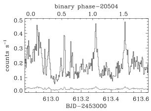
Figure 1.— MEG plus HEG count rate light curve of AE Aqr (black histogram) and $1\sigma$ error vector (lower gray histogram). Bin width $\Delta t=300$ s.

2.1. Light curve

Figure 1 shows the background-subtracted count rate light curve derived from the HETG event data. As has been well established by previous X-ray observations, the X-ray light curve of AE Aqr is dominated by flares, although this is by far the longest uninterrupted observation of AE Aqr and hence the clearest view of its X-ray light curve. During the Chandra observation, the flares last between a few hundred and a few thousand seconds, producing increases of up to 3–5 times the baseline count rate of $\sim 0.1~{}\rm counts~{}s^{-1}$.

Figure 2.— Soft (11–26 Å) over hard (1–8 Å) versus total (1–26 Å) count rate for AE Aqr (filled circles with error bars) and best-fitting constant function (dotted line) for the first three data points.

To constrain the cause and nature of the flares of AE Aqr, it is of interest to determine if the count rate variations shown in Figure 1 are accompanied by, or perhaps are even due to, dramatic variations in the X-ray spectrum. Previous investigations have indicated that this is not the case. For a flare observed by ASCA, Choi, Dotani, & Agrawal (1999) found no significant difference between the quiescent and flare X-ray spectra, although a “hint” of spectral hardening was recognized during the flare. For a flare observed by XMM-Newton, Choi & Dotani (2006) found that the X-ray spectrum at the beginning of the flare was similar to that in quiescence, but that the spectrum became harder as the flare advanced. Our ability to investigate spectral variations during the individual flares observed by Chandra is limited by the relatively low HETG count rate and the relatively fast timescale of the flares, although it is possible to investigate spectral variations for the ensemble of the flares. To accomplish this, the light curve shown in Figure 1 was divided into five count rate ranges: $I_{1}<0.14~{}\rm counts~{}s^{-1}$, $0.14\leq I_{2}<0.18~{}\rm counts~{}s^{-1}$, $0.18\leq I_{3}<0.23~{}\rm counts~{}s^{-1}$, $0.23\leq I_{4}<0.29~{}\rm counts~{}s^{-1}$, and $I_{5}\geq 0.29~{}\rm counts~{}s^{-1}$, where the count rate cuts were set to produce a roughly equal number of counts per count rate range, and the source and background counts were collected in three wavebands: hard (1–8 Å), medium (8–11 Å), and soft (11–26 Å), where the wavelength cuts were set to produce a roughly equal number of counts per wavelength interval. The background-subtracted soft $S$ over hard $H$ versus the total (1–26 Å) count rates are plotted in Figure 2. The dotted line in that figure is the best-fitting constant function $S/H=0.953$ for the first three data points (count rate ranges $I_{1}$–$I_{3}$). As shown by the figure, the softness ratio of the next higher count rate range $I_{4}$ is consistent with the lower ranges, while that of the highest count rate range $I_{5}$ is significantly ($3.6\sigma$) less. Consistent with the result of Choi & Dotani (2006), we find that the X-ray spectrum of the flares of AE Aqr is harder than that in quiescence only at the peak of the flares.

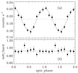
Figure 3.— (a) Spin-phase count rate light curve of AE Aqr (filled circles with error bars), best-fitting cosine function (solid curve), and mean count rate $A$ (dotted line). (b) Soft (11–26 Å) over hard (1–8 Å) spin-phase count rate light curve of AE Aqr (filled circles with error bars) and best-fitting constant function (solid line).

2.2. Spin-phase light curve

Figure 3a shows the background-subtracted spin-phase count rate light curve derived from the HETG event data. It is well fit ($\chi^{2}$ per degree of freedom $\equiv\chi_{\nu}^{2}=7.26/7=1.04$) by the cosine function $A+B\,\cos 2\pi(\phi_{\rm spin}-\phi_{0})$, with mean count rate $A=0.191\pm 0.002~{}\rm counts~{}s^{-1}$, semi-amplitude $B=0.031\pm 0.002~{}\rm counts~{}s^{-1}$ (hence, relative X-ray pulse semi-amplitude $B/A=16\%\pm 1\%$) and, consistent with the updated spin ephemeris (Mauche, 2006), phase offset $\phi_{0}=0.00\pm 0.01$ (throughout the paper, errors are $1\sigma$ or 68% confidence for one free parameter).

Figure 4.— Semi-amplitude $B$ versus mean count rate $A$ for the intensity-resolved spin-phase count rate light curves of AE Aqr (filled circles with error bars), best-fitting constant fit to $B/A$ (dotted line) and best-fitting linear fits to $B/A$ versus $A$ (dashed curve) and $B$ versus $A$ (solid line).

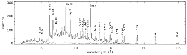
Figure 5.— MEG plus HEG count spectrum of AE Aqr (black histogram) and $1\sigma$ error vector (lower gray histogram). Bin width $\Delta\lambda=0.05$ Å. Emission lines used to construct the composite line profile are labeled.

The above result applies to the observation-average spin-phase light curve, although it is of interest to determine if the X-ray pulse semi-amplitude $B$ and/or the relative semi-amplitude $B/A$ varies with the mean count rate $A$. As for the investigation of the softness ratio variations, this is best determined as a function of time, using a time resolution sufficient to resolve the flares, but this is not possible with the relatively low count rate HETG data. Instead, background-subtracted spin-phase count rate light curves were derived from the HETG event data for each of the five count rate ranges defined above, and were then fit with the cosine function $A+B\,\cos 2\pi\phi_{\rm spin}$. The resulting values of the X-ray pulse semi-amplitude $B$ are plotted versus the mean count rate $A$ in Figure 4. The figure demonstrates that $B$ increases linearly with $A$ ($B/A$ is constant with $A$) in the middle of the count rate range, but that it saturates at both the low and high ends of the range; over the full count rate range, $B/A$ is not well fit ($\chi_{\nu}^{2}=5.82/4=1.46$) by a constant $B/A=0.162\pm 0.012$ (dotted line in Fig. 4). Instead, $B/A$ versus $A$ and $B$ versus $A$ are well fit by a linear relation $a+bA$ with, respectively, $a=0.22\pm 0.03$ and $b=-0.25\pm 0.15$, with $\chi_{\nu}^{2}=2.77/3=0.92$ (dashed curve in Fig. 4), and $a=0.011\pm 0.006$ and $b=0.10\pm 0.03$, with $\chi_{\nu}^{2}=2.38/3=0.79$ (solid line in Fig. 4).

To determine if the observed spin-phase flux modulation is due to photoelectric absorption (or some other type of broad-band spectral variability), background-subtracted spin-phase count rate light curves were derived from the HETG event data for each of three wavebands defined above: hard (1–8 Å), medium (8–11 Å), and soft (11–26 Å). Figure 3b shows the ratio of the resulting soft $S$ over hard $H$ spin-phase count rate light curves. The data is well fit ($\chi_{\nu}^{2}=7.20/9=0.80$) by a constant $S/H=0.916\pm 0.019$, which strongly constrains the cause of the observed spin-phase flux modulation. Specifically, if the observed flux modulation is caused by photoelectric absorption, a variation in the neutral hydrogen column density $\Delta N_{\rm H}\approx 3\times 10^{21}~{}\rm cm^{-2}$ is required, whereas the essential constancy of the softness ratio light curves requires $\Delta N_{\rm H}\lesssim 1\times 10^{20}~{}\rm cm^{-2}$; a factor of 30 times lower.

Table 1Line Fit Parameters, Flux Ratios, and Inferred Electron Densities.

	velocity	$\sigma$	Flux ($10^{-4}~{}\rm photons~{}cm^{-2}~{}s^{-1}$)						$\log n_{\rm e}$
Element	($\rm km~{}s^{-1}$)	(eV)	Lyman $\alpha$	$f$	$i$	$r$	$G=(f+i)/r$	$R^{\prime}=f/(i+r)$	($\rm cm^{-3}$)
O.	$-75\pm\phantom{0}51$	$1.12\pm 0.09$	$2.91\phantom{0}\pm 0.27$0	$0.35\phantom{0}\pm 0.17\phantom{0}$	$0.84\phantom{0}\pm 0.24\phantom{0}$	$1.12\phantom{0}\pm 0.26\phantom{0}$	$1.05\pm 0.35$	$0.178\pm 0.090$	$11.36_{-0.32}^{+0.42}$
Ne.	$+45\pm\phantom{0}53$	$2.02\pm 0.17$	$0.999\pm 0.073$	$0.206\pm 0.067$	$0.200\pm 0.064$	$0.622\pm 0.089$	$0.65\pm 0.18$	$0.251\pm 0.088$	$12.30_{-0.36}^{+0.35}$
Mg.	$+49\pm 104$	$3.85\pm 0.60$	$0.188\pm 0.019$	$0.070\pm 0.021$	$0.040\pm 0.020$	$0.193\pm 0.024$	$0.57\pm 0.17$	$0.300\pm 0.099$	$13.04_{-0.73}^{+0.45}$
Si.	$+95\pm 118$	$5.50\pm 0.90$	$0.185\pm 0.019$	$0.055\pm 0.014$	$0.028\pm 0.017$	$0.205\pm 0.020$	$0.41\pm 0.11$	$0.235\pm 0.065$	$14.14_{-0.36}^{+0.34}$

2.3. Spectrum

Figure 5 shows the background-subtracted count spectrum derived from the HETG event data, using $\Delta\lambda=0.05$ Å wavelength bins as a compromise between spectral resolution and sign-to-noise ratio. As is typical of unabsorbed cataclysmic variables (CVs) (Mukai et al., 2003; Mauche, 2007), the X-ray spectrum of AE Aqr is that of a multi-temperature thermal plasma, with emission lines of H- and He-like O, Ne, Mg, Si, and S and L-shell Fe XVII–Fe XXIV. However, unlike other CVs, and, in particular, unlike other magnetic CVs, the H-like Fe XXVI and He-like Fe XXV lines and the “neutral” fluorescent Fe K line are not apparent in the HETG spectrum. The apparent absence of these features in the HETG spectrum places limits on the maximum temperature of the plasma in AE Aqr and the amount of reflection from the surface of the white dwarf, although higher-energy instruments, such as those onboard Suzaku, are better suited to study this portion of the X-ray spectrum (see Terada et al., 2008).

We conducted a quantitative analysis of the X-ray spectrum of AE Aqr in three steps. First, Gaussians were fitted to the strongest emission lines of H- and He-like O, Ne, Mg, and Si to determine their radial velocities, widths, and fluxes. Second, a global model was fitted to the X-ray spectrum to constrain its absorbing column density, emission measure distribution, and elemental abundances. Third, using the emission measure distribution and the flux ratios of the He $\alpha$ forbidden ($f$), intercombination ($i$), and recombination ($r$) lines, constraints are placed on the density of the plasma.

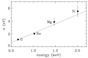
Figure 6.— Gaussian width $\sigma$ versus line energy for the Lyman $\alpha$ emission lines of H-like O, Ne, Mg, and Si (filled circles with error bars) and best-fitting linear function (solid line).

2.3.1 Line radial velocities, widths, and fluxes

The radial velocities, widths, and fluxes above the continuum of the Lyman $\alpha$ emission lines of O VIII, Ne X, Mg XII, and Si XIV and the He $\alpha$ triplets of O VII, Ne IX, Mg XI, and Si XIII were determined by fitting the flux in the MEG spectrum in the immediate vicinity of each emission feature with a constant plus one (Lyman $\alpha$) or three (He $\alpha$) Gaussians, employing the ARF and RMF files to account for the effective area of the spectrometer and its $\Delta\lambda=0.023$ Å [$690~{}\rm km~{}s^{-1}$ at 10 Å] FWHM spectral resolution. For each emission feature, the radial velocity was determined relative to the laboratory wavelengths from the Interactive Guide for ATOMDB version 1.3. More specifically, the assumed wavelengths for the Lyman $\alpha$ lines are the mean of the wavelengths of the doublets weighted by their relative emissivities (2:1), whereas the wavelengths for the He $\alpha$ intercombination lines are the unweighted means of their component $x$ and $y$ lines. In the fits to the He $\alpha$ triplets, the radial velocities and widths determined from the fits to the corresponding Lyman $\alpha$ lines were assumed, so that, in all cases, the fits had four free parameters. For these fits, unbinned data were employed and the C statistic (Cash, 1979) was used to determine the value of and error on the fit parameters, which are listed in Table 1. As demonstrated in Figure 6, we find that the widths of the Lyman $\alpha$ emission lines increase with the line energy, from $\sigma=1.1\pm 0.1$ eV for O VIII to $\sigma=5.5\pm 0.9$ eV for Si XIV. For comparison, during two flares of AE Aqr observed with the XMM-Newton Reflection Grating Spectrometer (RGS), Itoh et al. (2006) found $\sigma\approx 1.2$ and 2 eV for the Lyman $\alpha$ emission lines of N VII and O VIII, respectively. The trend shown in Figure 6 is well fit ($\chi_{\nu}^{2}=1.43/2=0.71$) with a linear function $a+bE$ with $a=-0.80\pm 0.29$ and $b=2.9\pm 0.4$. Consistent with the non-zero intercept $a$, the line widths are not constant in velocity units, but increase with the line energy: $\sigma=512\pm 39$, $593\pm 51$, $784\pm 121$, and $822\pm 135~{}\rm km~{}s^{-1}$ for O VIII, Ne X, Mg XII, and Si XIV, respectively. In addition to the line widths, there is some evidence that the radial velocities of the Lyman $\alpha$ emission lines increase with the line energy, from $v=-75\pm 51~{}\rm km~{}s^{-1}$ for O VIII to $v=+95\pm 118~{}\rm km~{}s^{-1}$ for Si XIV. Note, however, that the velocity difference, $\Delta v=170\pm 128~{}\rm km~{}s^{-1}$, differs from zero by just $1.3\sigma$, is a small fraction of the widths of the lines, and is probably affected by systematic effects. If a common radial velocity offset is assumed in the fits of the Lyman $\alpha$ lines, the derived velocity $v=-1\pm 33~{}\rm km~{}s^{-1}$.

2.3.2 Global model

To produce a global model of the X-ray spectrum of AE Aqr, ATOMDB IDL version 2.0.0 software was used to construct ATOMDB version 1.3.1 optically-thin thermal plasma X-ray spectral models for the continuum and for the 12 cosmically abundant elements C, N, O, Ne, Mg, Al, Si, S, Ar, Ca, Fe, and Ni at 40 temperatures spaced uniformly in $\log T$ [specifically, $\log T({\rm K})=5.0,5.1,5.2,\ldots,8.9$]. Using custom IDL software, these spectral eigenvectors were convolved with a Gaussian, to account for the observed widths of the emission lines as a function of temperature, and multiplied by the grating ARFs and RMFs, to account for the spectrometer’s effective area and spectral resolution. The resulting $\pm$ first-order MEG and HEG spectral models were then binned to 0.05 Å and coadded. Finally, the observed MEG plus HEG count spectrum (Fig. 5) and whence the spectral models were “grouped” to a minimum of 30 counts per bin so that Gaussian statistics could be used in the fits.

Numerous model emission measure ($EM$) distributions were tested against the data: 1, 2, 3, and 4 single-temperature models, a cut-off power law ($dEM/d\log T\propto T^{\alpha}$ for $T\leq T_{\rm c}$), a power law with an exponential cutoff ($dEM/d\log T\propto T^{\alpha}$ for $T\leq T_{\rm c}$ and $dEM/d\log T\propto T^{\alpha}\exp[(T_{\rm c}-T)/T_{\rm f}]$ for $T>T_{\rm c}$), and a Gaussian ($dEM/d\log T\propto\exp[-(\log T-\log T_{0})^{2}/2\sigma^{2}]$), all with photoelectric absorption by a neutral column (Morrison & McCammon, 1983) and variable elemental abundances relative to those of Anders & Grevesse (1989).

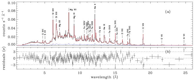
Figure 7.— (a) MEG plus HEG spectrum of AE Aqr (black histogram), $1\sigma$ error vector (lower blue histogram), and the best-fit ATOMDB absorbed variable-abundance Gaussian emission measure distribution model (red histogram). (b) Corresponding residuals.

Among these models, the best (if not a particularly good) fit ($\chi_{\nu}^{2}=382.7/233=1.64$) was achieved with a model with a Gaussian emission measure distribution with a peak temperature $\log T_{0}({\rm K})=7.16\pm 0.01$, a width $\sigma=0.48\pm 0.01$, an absorbing column density $N_{\rm H}=(1.0\pm 0.6)\times 10^{20}~{}\rm cm^{-2}$, an Fe abundance equal to $0.44\pm 0.02$ times solar, and the other metal abundances equal to $0.76\pm 0.03$ times solar. The X-ray spectrum of this model is shown superposed on the data in Figure 7. For an assumed distance $d=100$ pc (Friedjung, 1997), the total emission measure $EM=8.8\times 10^{53}~{}\rm cm^{-3}$ and the unabsorbed 0.5–10 keV luminosity $L_{\rm X}=1.1\times 10^{31}~{}\rm erg~{}s^{-1}$; if this luminosity is due to accretion onto the white dwarf, the mass accretion rate $\dot{M}=L_{\rm X}R_{\rm wd}/GM_{\rm wd}\approx 7.3\times 10^{13}~{}\rm g~{}s^{-1}$.

Before leaving this section, it is useful to note that the Gaussian emission measure distribution derived above extends over nearly two orders of magnitude in temperature — from $T\approx 1.6\times 10^{6}$ K to $1.3\times 10^{8}$ K at $\pm 2\sigma$ — but peaks at a temperature $T\approx 1.4\times 10^{7}$ K or 1.2 keV. Such a low temperature is uncharacteristic of CVs, and in particular magnetic CVs: note for instance that AE Aq had the lowest continuum temperature of any magnetic CV observed by ASCA (Ezuka & Ishida, 1999). The characteristic temperatures of magnetic CVs are the shock temperature, $T_{\rm s}=3\mu m_{\rm H}GM_{\rm wd}/8kR_{\rm wd}\approx 4.1\times 10^{8}$ K or 35 keV, applicable for radial free-fall onto the white dwarf, and the blackbody temperature, $T_{\rm bb}=(L_{\rm X}/\sigma A)^{1/4}\approx 19\,(f/0.25)^{-1/4}$ kK (where the radiating area $A=4\pi R_{\rm wd}^{2}f$ and our choice for the fiducial value of the fractional emitting area $f$ will be justified in §4.1), applicable for deposition of the accretion luminosity in the surface layers of the white dwarf (e.g., bombardment or blobby accretion). The only evidence for plasma at the shock temperature is supplied by the Suzaku X-ray spectrum of AE Aqr, but Terada et al. (2008) argued strongly for a nonthermal origin for this emission. The blackbody temperature, on the other hand, is close to the temperature of the hot spots that Eracleous et al. (1994) derived from the maximum entropy maps of the UV pulse profiles of AE Aqr. More on this below.

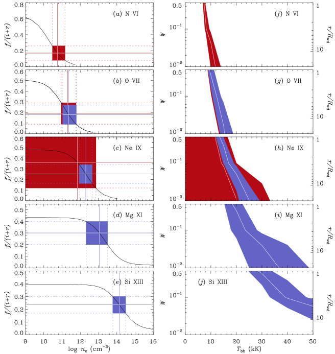
Figure 8.— (a)–(e): $R^{\prime}=f/(i+r)$ flux ratio versus $\log n_{\rm e}$ for N VI, O VII, Ne IX, Mg XI, and Si XIII for $T_{\rm bb}=0$ and $\log T_{\rm e}({\rm K})=6.2$, 6.4, 6.6, 6.8, and 7.0, respectively. Observed flux ratios and errors are from Table 4 of Itoh et al. (2006) (red horizontal lines) and Table 1 of this paper (blue horizontal lines); the inferred electron densities and errors (colored vertical lines) are listed in Table 1. Colored boxes delineate the $1\sigma$ error envelope of the flux ratio and $\log n_{\rm e}$ for each ion. (f)–(j): Corresponding contours of the observed $R^{\prime}$ flux ratios (white curves) and $1\sigma$ error envelops (colored polygons) for $n_{\rm e}=1~{}\rm cm^{-3}$ as a function of $T_{\rm bb}$ and $W$.

2.3.3 Plasma densities

We now consider in more detail the forbidden ($f$), intercombination ($i$), and recombination ($r$) line fluxes of the He $\alpha$ triplets of O VII, Ne IX, Mg XI, and Si XIII derived in §2.3.1 and listed in Table 1. As elucidated by Gabriel & Jordan (1969); Blumenthal, Drake, & Tucker (1972); and Porquet et al. (2001), these line fluxes can be used to constrain the electron temperature $T_{\rm e}$ via the $G=(f+i)/r$ flux ratio and the electron density $n_{\rm e}$ via the $R=f/i$ flux ratio of each He-like ion. Because the errors on the observed $R$ flux ratios are large, we follow Itoh et al. (2006) and employ the $R^{\prime}=f/(i+r)$ flux ratio as an electron density diagnostic in the subsequent discussion. The observed $G$ and $R^{\prime}$ flux ratios and errors are listed in Table 1. To interpret these results, we derived the $R^{\prime}=RG/(1+R+G)$ flux ratios from the $G$ and $R$ flux ratios tabulated by Porquet et al. (2001) for a collisional plasma for N VI, O VII, Ne IX, Mg XI, and Si XIII for $\log T_{\rm e}({\rm K})=6.2$, 6.4, 6.6, 6.8, and 7.0, respectively, where the temperatures are those of the peaks of the He-like triplet emissivities weighted by the Gaussian emission measure distribution, determined in the previous section from the global fit to the X-ray spectrum. With the exception of Si XIII, in each case the assumed electron temperature is consistent with the observed $G$ flux ratio. With these assumptions, the theoretical values of $R^{\prime}$ are shown in the left panels of Figure 8 as a function of $\log n_{\rm e}$. In addition to the $R^{\prime}$ flux ratios of O VII, Ne IX, Mg XI, and Si XIII measured from the Chandra HETG spectrum (Table 1), we added to Figure 8 the $R^{\prime}$ flux ratios of N VI, O VII, and Ne IX measured by Itoh et al. from the XMM-Newton RGS spectrum of AE Aqr. Figure 8(b) of this paper corrects an error in Figure 5(h) of Itoh et al., which showed the $R^{\prime}$ flux ratio extending from 0.09 to 0.39, whereas the data in their Table 4 shows that it should extend only to 0.29. With this correction, the RGS- and HETG-derived values of and errors on the $R^{\prime}$ flux ratio of O VII are nearly identical. This correction, the significantly smaller error range on the $R^{\prime}$ flux ratio of Ne IX, and the HETG results for Mg XI and Si XIII indicates that, contrary to the conclusion of Itoh et al., the electron density of the plasma in AE Aqr increases with temperature by over three orders of magnitude, from $n_{\rm e}\approx 6\times 10^{10}~{}\rm cm^{-3}$ for N VI [$\log T_{\rm e}({\rm K})\approx 6.2$] to $n_{\rm e}\approx 1\times 10^{14}~{}\rm cm^{-3}$ for Si XIII [$\log T_{\rm e}({\rm K})\approx 7.0$].

In addition to electron density, the $R$ and hence the $R^{\prime}$ flux ratio is affected by photoexcitation, so we must investigate the sensitivity of the $R^{\prime}$ flux ratios to an external radiation field. To investigate the conditions under which a low-density plasma can masquerade as a high-density plasma, we derived the $R^{\prime}$ flux ratios from the $G$ and $R$ flux ratios tabulated by Porquet et al. (2001) for a low-density ($n_{\rm e}=1~{}\rm cm^{-3}$) collisional plasma irradiated by a blackbody with temperature $T_{\rm bb}$ and dilution factor $W$. Under the assumption that this flux originates from the surface of the white dwarf, $W={1\over 2}\ \{1-[1-(R_{\rm wd}/r)]^{1/2}\}$, where $r$ is the distance from the center of the white dwarf, hence $W={1\over 2}$ on the white dwarf surface. In the right panels of Figure 8 we show contours of the observed $R^{\prime}$ flux ratios (white curves) and $1\sigma$ error envelops (colored polygons) of the various He-like ions as a function of $T_{\rm bb}$ and $W$. The figure demonstrates that the observed $R^{\prime}$ flux ratios of N VI, O VII, Ne IX, Mg XI, and Si XIII can be produced in a low-density plasma sitting on the white dwarf surface if the blackbody temperature $T_{\rm bb}\approx 7$, 10, 14, 18, and 30 kK, respectively, or at higher temperatures at greater distances from the white dwarf. Conversely, the figure gives the allowed range of distances (dilution factors) for each ion for a given blackbody temperature. For example, for $T_{\rm bb}=25$ kK, the volume of plasma in which Si XIII dominates [$\log T({\rm K})\approx 7.0$] could be on the white dwarf surface, while that of Mg XI [$\log T({\rm K})\approx 6.8$] would have to be at $r\approx 3\,R_{\rm wd}$, that of Ne X [$\log T({\rm K})\approx 6.6$] would have to be at $r\approx 20\,R_{\rm wd}$, and so on for the lower Z ions.

2.4. Radial velocities

In the next component of our analysis, we used two techniques to search for orbit- and spin-phase radial velocity variations in the X-ray emission lines of AE Aqr.

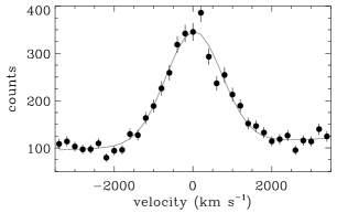
Figure 9.— MEG plus HEG composite line profile of AE Aqr (filled circles with error bars) and best-fitting Gaussian function (solid curve).

2.4.1 Composite line profile technique

In the first technique, similar to that employed by Hoogerwerf, Brickhouse, & Mauche (2004), phase-average as well as orbit- and spin-phase resolved composite line profiles were formed by coadding the HETG event data in velocity space $v=c(\lambda-\lambda_{0})/\lambda$ relative to laboratory wavelengths $\lambda_{0}$ from the Interactive Guide for ATOMDB version 1.3. The lines used in this analysis are those labeled in Figures 5 and 7 shortward of 20 Å. For the H-like lines, the wavelengths are the mean of the wavelengths of the doublets weighted by their relative emissivities (2:1), while for the He-like lines, the wavelengths are for the stronger resonance lines. The resulting phase-average composite line profile is shown in Figure 9. Fit with a Gaussian, its offset $v=25\pm 26~{}\rm km~{}s^{-1}$ and width $\sigma=712\pm 27~{}\rm km~{}s^{-1}$.

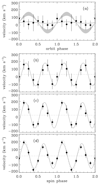
Figure 10.— Orbit- and spin-phase radial velocities of the X-ray emission lines of AE Aqr. Four panels show the data (filled circles with error bars), best-fitting sine function (solid curve), and $\gamma$ velocity (dotted line) for (a) and (b) the composite line technique, (c) the cross correlation technique, and (d) the cross correlation technique using the boost-strapped template spectrum. Shaded region in the upper panel is the $1\sigma$ error envelope of the expected white dwarf orbit-phase radial velocity variation.

Applying the composite line profile technique to the orbit-phase resolved composite line profiles results in the radial velocities shown in Figure 10a. Assuming that, like EX Hya (Hoogerwerf, Brickhouse, & Mauche, 2004), the orbit-phase radial velocities follow the motion of the white dwarf, these data are well fit ($\chi_{\nu}^{2}=1.29/6=0.22$) by the sine function

$$v(\phi_{\rm orb})=\gamma+K{1\over\Delta}\int^{\phi_{\rm orb}+\Delta/2}_{\phi_{\rm orb}-\Delta/2}\sin 2\pi\phi\,d\phi,$$ (1)

where $\Delta=1/8$, with $\gamma=30\pm 25~{}\rm km~{}s^{-1}$ and $K=12\pm 36~{}\rm km~{}s^{-1}$ (solid curve in Fig. 10a), although they are slightly better fit ($\chi_{\nu}^{2}=1.41/7=0.20$) with a constant $\gamma=29\pm 25~{}\rm km~{}s^{-1}$. For future reference, we note that the $1\sigma$, $2\sigma$, and $3\sigma$ ($\Delta\chi^{2}=1.0$, 2.71, and 6.63) upper limits to the orbit-phase radial velocity semi-amplitude $K=48$, 72, and $105~{}\rm km~{}s^{-1}$, respectively.

Applying the composite line profile technique to the spin-phase resolved composite line profiles results in the radial velocities shown in Figure 10b. Unlike the orbit-phase radial velocities, these data are not well fit ($\chi_{\nu}^{2}=18.3/7=2.6$) by a constant, but they are well fit ($\chi_{\nu}^{2}=2.85/5=0.57$) by the sine function

$$v(\phi_{\rm spin})=\gamma+K{1\over\Delta}\int^{\phi_{\rm spin}+\Delta/2}_{\phi_{\rm spin}-\Delta/2}\sin 4\pi(\phi-\phi_{0})\,d\phi,$$ (2)

where $\Delta=1/8$, with $\gamma=29\pm 25~{}\rm km~{}s^{-1}$, $K=149\pm 38~{}\rm km~{}s^{-1}$, and $\phi_{0}=0.060\pm 0.021$ (solid curve in Fig. 10b).

2.4.2 Cross correlation technique

The composite line profile technique employed above utilizes the strongest isolated emission lines in the HETG spectrum of AE Aqr, ignoring the many weaker and often blended spectral features shown in Figures 5 and 7. In an attempt to reduce the size of the error bars on the derived spin-phase radial velocities, a cross correlation technique was tested. To accomplish this, spin-phase resolved spectra were formed by adding the HETG event data in wavelength space using bins of constant velocity width $\Delta v=100~{}\rm km~{}s^{-1}$ (specifically, $\lambda=3.000,3.001,3.002,\ldots 25.002$ Å). In the absence of an obvious template against which to cross correlate the resulting spin-phase resolved spectra, the spectrum from the first spin phase bin, $\phi_{\rm spin}=0\pm\Delta/2$, was used as the template. The resulting spin-phase radial velocities, shown in Figure 10c, are very similar to those derived using the composite line technique (Fig. 10b), but the error bars are smaller by a factor of approximately 40%. These data are reasonably well fit ($\chi_{\nu}^{2}=4.75/4=1.19$) by equation 2 with $\gamma=22\pm 15~{}\rm km~{}s^{-1}$, $K=167\pm 23~{}\rm km~{}s^{-1}$, and $\phi_{0}=0.045\pm 0.012$ (solid curve in Fig. 10c). Note that, given the manner in which this result was derived, the $\gamma$ velocity is now relative that of the template, the spectrum from the first spin phase, for which the composite line profile technique gave a radial velocity $v=-1\pm 57~{}\rm km~{}s^{-1}$ (i.e., consistent with zero).

Given this fit to the radial velocities of the spin-phase resolved spectra, it is possible to produce a spin-phase average spectrum that accounts for (removes the effect of) the spin-phase radial velocities. This was accomplished by multiplying the wavelengths of the HETG event data by a factor $1-v(\phi_{\rm spin})/c$, where $v(\phi_{\rm spin})=\gamma+K\,\sin 4\pi(\phi_{\rm spin}-\phi_{0})~{}\rm km~{}s^{-1}$ with parameters that are equal to the previous best-fit values: $\gamma=22~{}\rm km~{}s^{-1}$, $K=167~{}\rm km~{}s^{-1}$, and $\phi_{0}=0.045$. The spin-phase radial velocities derived using the resulting boot-strapped spin-phase average spectrum as the cross correlation template are shown in Figure 10d. They are very similar to the radial velocities derived using the “vanilla” cross correlation technique (Fig. 10c), but the error bars are smaller by a factor of approximately 30%. These data are now not particularly well fit ($\chi_{\nu}^{2}=10.3/5=2.1$) by equation 2 with $\gamma=15\pm 10~{}\rm km~{}s^{-1}$, $K=163\pm 15~{}\rm km~{}s^{-1}$, and $\phi_{0}=0.022\pm 0.008$ (solid curve in Fig. 10d). The deviations from the fit appear to be consistent with a radial velocity amplitude that is larger on the 0–0.5 spin-phase interval and smaller on the 0.5–1 spin-phase interval. Accordingly, equation 2 was modified to allow this additional parameter, and the data are then well fit ($\chi_{\nu}^{2}=0.82/4=0.21$) with $\gamma=14\pm 10~{}\rm km~{}s^{-1}$, $K_{1}=206\pm 20~{}\rm km~{}s^{-1}$ (valid on $\phi_{\rm spin}=0$–0.5), $K_{2}=120\pm 20~{}\rm km~{}s^{-1}$ (valid on $\phi_{\rm spin}=0.5$–1), and $\phi_{0}=0.023\pm 0.008$ (dotted curve in Fig. 10d).

3. Summary

As summarized below, our long, uninterrupted Chandra HETG observation provides a wealth of details concerning the X-ray emission of AE Aqr:

1. The X-ray light curve is dominated by flares that last between a few hundred and a few thousand seconds, produce increases of up to 3–5 times the baseline count rate (Fig. 1), and are achromatic except near their peaks (Fig. 2); the white dwarf spin-phase X-ray light curve is achromatic and sinusoidal in shape, with a relative semi-amplitude of approximately $16\%$ (Fig. 3); and the X-ray pulse amplitude increases linearly with the mean count rate in the middle of the range, but saturates at both the low and high ends of the range (Fig. 4).

2. The X-ray spectrum is that of an optically thin multi-temperature thermal plasma (Fig. 5); the X-ray emission lines are broad (Fig. 9), with widths that increase with the line energy, from $\sigma\approx 1$ eV ($510~{}\rm km~{}s^{-1}$) for O VIII to $\sigma\approx 5.5$ eV ($820~{}\rm km~{}s^{-1}$) for Si XIV (Fig. 6); the X-ray spectrum is reasonably well fit by a plasma model with a Gaussian emission measure distribution that peaks at $\log T({\rm K})=7.16$, has a width $\sigma=0.48$, an Fe abundance equal to $0.44$ times solar, and other metal (primarily Ne, Mg, and Si) abundances equal to $0.76$ times solar (Fig. 7); and for a distance $d=100$ pc, the total emission measure $EM=8.0\times 10^{53}~{}\rm cm^{-3}$ and the 0.5–10 keV luminosity $L_{\rm X}=1.1\times 10^{31}~{}\rm erg~{}s^{-1}$.

3. Based on the $f/(i+r)$ flux ratios of the He $\alpha$ triplets of N VI, O VII, Ne IX measured by Itoh et al. in the XMM-Newton Reflection Grating Spectrometer spectrum, and those of O VII, Ne IX, Mg XI, and Si XIII in the Chandra HETG spectrum, the electron density of the plasma increases with temperature by over three orders of magnitude, from $n_{\rm e}\approx 6\times 10^{10}~{}\rm cm^{-3}$ for N VI [$\log T_{\rm e}({\rm K})\approx 6.2$] to $n_{\rm e}\approx 1\times 10^{14}~{}\rm cm^{-3}$ for Si XIII [$\log T_{\rm e}({\rm K})\approx 7.0$] (Table 1 and Fig. 8a–e), and/or the plasma is significantly affected by photoexcitation (Fig. 8f–j).

4. The radial velocity of the X-ray emission lines varies on the white dwarf spin phase, with two oscillations per spin cycle and an amplitude $K\approx 160~{}\rm km~{}s^{-1}$ (Fig. 10).

4. Discussion

Over the years, two very different models have been proposed for the source of the X-ray emission of AE Aqr. On one hand, based on ROSAT and ASCA data, Eracleous (1999) argued that the X-ray emission, including the flares, must occur close to the white dwarf, so that the gravitational potential energy can heat the X-ray emitting plasma to the observed temperatures. Similarly, based on Ginga and ASCA data, Choi, Dotani, & Agrawal (1999) argued that the X-ray emission, both persistent and flare, originates within the white dwarf magnetosphere; Choi & Dotani (2006) came to similar conclusions based on XMM-Newton Optical Monitor (OM) and European Photon Imaging Camera (EPIC) data. On the other hand, based on XMM-Newton RGS data, Itoh et al. (2006) argued that the $f/(i+r)$ flux ratios of the He $\alpha$ triplets of N VI, O VII, and Ne IX are consistent with a plasma with an electron density $n_{\rm e}\sim 10^{11}~{}\rm cm^{-3}$ and, given the observed emission measure, a linear scale $l\approx(2$–$3)\times 10^{10}$ cm. Because this density is orders of magnetic less than the conventional estimate for the post-shock accretion column of a magnetic CV, and because this linear scale is much larger than the radius of the white dwarf, these authors argued that the optically thin X-ray-emitting plasma in AE Aqr is due not to accretion onto the white dwarf, but to blobs in the accretion stream, heated to X-ray emitting temperatures by the propeller action of the white dwarf magnetic field. Ikhsanov (2006) has taken issue with some of the details of this model, arguing that the detected X-rays are due to either (1) a tenuous component of the accretion stream or (2) plasma “outside the system,” heated by accelerated particles and/or MHD waves due to a pulsar-like mechanism powered by the spin-down of the magnetic white dwarf. The presence of non-thermal particles in AE Aqr is supported by the observed TeV $\gamma$-rays and the recent discovery by Terada et al. (2008) of a hard, possibly power-law, component in the Suzaku X-ray spectrum of AE Aqr. Finally, Venter & Meintjes (2007) have proposed that the observed unpulsed X-ray emission in AE Aqr is the result of a very tenuous hot corona associated with the secondary star, which is pumped magnetohydrodynamically by the propeller action of the white dwarf magnetic field. As we argue below, the results of our Chandra HETG observation of AE Aqr — particularly the orbit-phase pulse time delays, the high electron densities and/or high levels of photoexcitation implied by the He $\alpha$ triplet flux ratios, and the large widths and spin-phase radial velocities of the X-ray emission lines — are not consistent with an extended, low-density source of X-rays in AE Aqr, but instead support earlier models in which the dominant source of X-rays is of high density and/or in close proximity to the white dwarf.

Consider first the systemic velocity of the X-ray emission lines. We variously measured this quantity to be $v=-1\pm 33~{}\rm km~{}s^{-1}$ from the Lyman $\alpha$ emission lines (§2.3.1), $v=25\pm 26~{}\rm km~{}s^{-1}$ from the composite line profile (Fig. 9), $\gamma=29\pm 25~{}\rm km~{}s^{-1}$ from the composite line profile fit to the radial velocities (Fig. 10b), and $\gamma=22\pm 15~{}\rm km~{}s^{-1}$ from the cross correlation fit to the radial velocities (Fig. 10c). Optimistically assuming that these measurements are neither correlated nor strongly affected by systematic effects, the weighted mean and standard deviation of the systemic velocity of the X-ray emission lines $\gamma_{\rm X}=21\pm 11~{}\rm km~{}s^{-1}$. Relative to the systemic velocity of the optical emission (absorption) lines, $\gamma_{\rm O}\approx-38\pm 9\>(-64\pm 11)~{}\rm km~{}s^{-1}$ (Robinson et al., 1991; Reinsch & Beuermann, 1994; Welsh et al., 1995; Casares et al., 1996; Watson et al., 2006), the X-ray emission lines are redshifted by $\Delta v=\gamma_{\rm X}-\gamma_{\rm O}\approx 59\pm 14~{}(85\pm 16)~{}\rm km~{}s^{-1}$. This result is to be compared to the free-fall velocity $v_{\rm ff}=(2GM_{\rm wd}/R_{\rm wd})^{1/2}\approx 5500~{}\rm km~{}s^{-1}$ onto the surface of the white dwarf, the infall velocity $v_{\rm in}\leq v_{\rm ff}/4\approx 1375~{}\rm km~{}s^{-1}$ below the putative standoff shock, and the gravitational redshift $\Delta v=GM_{\rm wd}/R_{\rm wd}c=51^{+13}_{-11}~{}\rm km~{}s^{-1}$ from the surface of the white dwarf with a mass $M_{\rm wd}=0.8\pm 0.1~{}\rm M_{\odot}$ and radius $R_{\rm wd}=(7.0\mp 0.8)\times 10^{8}$ cm (Robinson et al., 1991; Welsh et al., 1993; Reinsch & Beuermann, 1994; Welsh et al., 1995; Casares et al., 1996; Watson et al., 2006). Although the determination and interpretation of systemic velocities is fraught with uncertainties, the systemic velocity of the X-ray emission lines of AE Aqr is consistent with the gravitational redshift from the surface of the white dwarf, and hence with a source on or near the surface of the white dwarf, rather than a more extended region within the binary.

Supporting the proposal that the X-ray emission of AE Aqr is closely associated with the white dwarf is the fact, established previously by Mauche (2006), that the X-ray spin pulse follows the motion of the white dwarf around the binary center of mass, producing a time delay $\Delta t=2.17\pm 0.48$ s in the arrival times of the X-ray pulses. Given this result, it is somewhat surprising that the radial velocity of the X-ray emission lines does not appear to vary on the white dwarf orbit phase: the measured orbit-phase radial velocity semi-amplitude $K=12\pm 36~{}\rm km~{}s^{-1}$, whereas the expected value $K=2\pi\Delta tc/P_{\rm orb}=115\pm 25~{}\rm km~{}s^{-1}$ (Fig. 10a). The difference between the measured and expected radial velocity semi-amplitudes is $103\pm 44~{}\rm km~{}s^{-1}$, which differs from zero by $2.3\sigma$. While this discrepancy is of some concern, we showed above that the radial velocity of the X-ray emission lines varies on the white dwarf spin phase (Fig. 10b–d), which argues strongly for a source of X-rays trapped within, and rotating with, the magnetosphere of the white dwarf.

In contrast, it seems clear that our result for the radial velocity of the X-ray emission lines is not consistent with the proposal, put forward by Itoh et al. (2006), that the accretion stream is the dominant source of X-rays in AE Aqr. For the system parameters of AE Aqr, the accretion stream makes its closest approach to the white dwarf at a radius $r_{\rm min}\approx 1\times 10^{10}$ cm and a velocity $v_{\rm max}\approx 1500~{}\rm km~{}s^{-1}$. Accounting for the binary inclination angle $i=60^{\circ}$, the predicted accretion stream radial velocity amplitude $v_{\rm max}\sin i\approx 1300~{}\rm km~{}s^{-1}$, whereas the $3\sigma$ upper limit to the orbit-phase radial velocity semi-amplitude $K=105~{}\rm km~{}s^{-1}$. Clearly, the accretion stream, if it follows a trajectory anything like the inhomogeneous diamagnetic accretion flow calculated by Wynn, King, & Horne (1997), cannot be the dominant source of X-rays in AE Aqr.

An additional argument against the accretion stream (Itoh et al., 2006), plasma “outside the system” (Ikhsanov, 2006), a hot corona associated with the secondary star (Venter & Meintjes, 2007), or any other extended source of X-rays in AE Aqr is the high electron densities $\log n_{\rm e}\approx 10.8$, 11.4, 12.3, 13.0, and 14.1 inferred from the $f/(i+r)$ flux ratios of the He $\alpha$ triplets of N VI, O VII, Ne IX, Mg XI, and Si XIII, respectively. Given the differential emission measure distribution $dEM/d\log T\approx 6.6\times 10^{53}\,\exp[-(\log T-\log T_{0})^{2}/2\sigma^{2}]$ with $\log T_{0}({\rm K})\approx 7.16$ and $\sigma\approx 0.48$, the N VI, O VII, Ne IX, Mg XI, and Si XIII He $\alpha$ triplet emissivity-weighted emission measure $EM=\int(dEM/d\log T)\,\varepsilon\,d\log T/\int\varepsilon\,d\log T\approx[0.9,1.6,3.3,4.8,5.8]\times 10^{52}~{}\rm cm^{-3}$ and the linear scale $l=(EM/n_{\rm e}^{2})^{1/3}\approx 1.4\times 10^{10}$, $6.7\times 10^{9}$, $2.0\times 10^{9}$, $7.4\times 10^{8}$, and $1.4\times 10^{8}$ cm or 20, 10, 3, 1, and $0.2~{}R_{\rm wd}$, respectively. Although even the observed Si XIII $f/(i+r)$ flux ratio can be produced in a low-density plasma suffering photoexcitation by an external radiation field, this requires both high blackbody temperatures ($T_{\rm bb}\gtrsim 25$ kK) and large dilution factors ($W\lesssim{1\over 2}$), hence small-to-zero distances above the white dwarf surface. We conclude that, if the bulk of the plasma near the peak of the emission measure distribution is not of high density, it must be in close proximity to the white dwarf.

4.1. White dwarf

To investigate the possibility that the X-rays observed in AE Aqr are associated with the white dwarf, we considered a simple geometric model, similar to that derived by Eracleous et al. (1994) from the maximum entropy maps of the UV pulse profiles measured with the Faint Object Spectrograph onboard the Hubble Space Telescope. The model consists of a rotating white dwarf viewed at an inclination angle $i=60^{\circ}$ from the rotation axis $\hat{z}$ with two bright spots, centered $20^{\circ}$ above and below the equator and separated in longitude by $180^{\circ}$ (i.e., the upper and lower spots are centered at spherical coordinates $[\theta,\phi]=[70^{\circ},0^{\circ}]$ and $[110^{\circ},180^{\circ}]$, respectively). Such a model naturally produces two unequal flux peaks per spin cycle, with the brighter (dimmer) peak occurring when the upper (lower) spot is pointed toward the observer. Instead of the optically thick assumption applied in the optical and UV, we assume that the X-ray emitting spots are optically thin. In this case, the X-ray flux modulation is produced solely by occultation by the body of the white dwarf, so the brightness of the lower spot must be reduced by approximately 30% to avoid producing a second peak in the X-ray light curve. Assuming that the brightness distribution of the spots is given by a Gaussian function $\exp(-\delta\theta^{2}/2\sigma^{2})$, where $\delta\theta$ is the polar angle from the center of the spot and the spot width $\sigma=30^{\circ}$ (hence $\rm FWHM=70^{\circ}$ and the fractional emitting area $f=\int\exp(-\theta^{2}/2\sigma^{2})\sin\theta d\theta\approx 0.25$, justifying our choice for the fiducial value of this quantity in §2.3.2), the light curves of the upper spot, the lower spot, and the total flux are as shown in Figure 11a. Smaller spots produce squarer light curves, while larger spots produce lower relative oscillation amplitudes; the relative pulse semi-amplitude of the model shown, $(I_{\rm max}-I_{\rm min})/(I_{\rm max}+I_{\rm min})=16\%$, is consistent with observations (Fig. 3a). The flux-weighted mean radial velocities of the emission from the upper spot, the lower spot, and the total flux are as shown in Figure 11b for an assumed white dwarf rotation velocity $v_{\rm rot}=2\pi R_{\rm wd}/P_{33}=1330~{}\rm km~{}s^{-1}$. As observed, the predicted radial velocity of the total flux goes through two oscillations per spin cycle, although the two peaks are not equal in strength, the red-to-blue zero velocity crossings do not occur near $\phi_{\rm spin}=0.25$ and 0.75, and the maximum velocity amplitude is greater than observed (Fig. 10b–d). Although it is possible to remedy these deficiencies by using two bright spots that are more nearly equal in brightness, this significantly reduces the pulse amplitude of the total flux. Furthermore, the model predicts that the width of the X-ray emission lines should be narrower near $\phi_{\rm spin}=0$ and 0.5 and broader near $\phi_{\rm spin}=0.25$ and 0.75, which is not corroborated by the data. Finally, the model predicts that the radial velocity amplitude of the total flux is higher (lower) on the 0.75–1.25 (0.25–0.75) spin phase interval, whereas the boot-strapped cross correlation technique provides evidence that this is the case approximately one quarter of a cycle later: on the 0–0.5 (0.5–1) spin phase interval (ignoring the small phase offset).

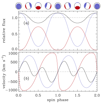
Figure 11.— Spin-phase (a) light curves and (b) radial velocities for the two-spot model of AE Aqr. Blue, red, and black curves are for the upper spot, the lower spot, and the total flux, respectively. Flux is relative to the total mean and velocities assume $v_{\rm rot}=1330~{}\rm km~{}s^{-1}.$ Upper graphic shows a schematic of the model at $\phi_{\rm spin}=0,0.25,0.5,\ldots 2$.

4.2. Accretion Columns

To place their results in a theoretical framework, Eracleous et al. (1994) interpreted the hot spots derived from their maximum entropy maps as the result of reprocessing of X-rays emitted by the post-shock gas in the accretion columns of a magnetic white dwarf. For an assumed point source of illumination, they found good fits to the UV pulse profiles if the angle between the spin axis and the magnetic axis — the magnetic colatitude — $\beta=76^{\circ}\pm 1^{\circ}$, the peak spot temperature $T_{\rm max}=26\pm 2$ kK, the height of the illuminating source above the white dwarf surface $H/R_{\rm wd}=3\pm 1$, and the X-ray luminosity $L_{\rm X}=3\times 10^{33}\,(H/3)^{2}\,(\eta/0.5)^{-1}~{}\rm erg~{}s^{-1}$, where $\eta$ is the efficiency of conversion of accretion luminosity into 0.1–4 keV X-rays (note that our fiducial value for this quantity is larger by an order of magnitude than that assumed by Eracleous et al. because the mean temperature of the X-ray spectrum of AE Aqr is uncharacteristically low). These results are troubling for two reasons. First, as noted by Eracleous et al., the shock height required to produce the size of the UV spots is quite large (comparable to the corotation radius). Second, the X-ray luminosity required to heat the 26 kK spots by reprocessing is more than two orders of magnitude greater than observed in the 0.5–10 keV bandpass. Adding to these problems, we found that such a model reproduces neither the X-ray pulse profile nor the radial velocity variation observed in AE Aqr. First, the predicted pulse profile has a square waveform, with the X-ray flux rapidly doubling (halving) when one of the illuminating spots emerges from (is hidden behind) the body of the white dwarf. Second (if the illuminating spots are not equal in brightness), the predicted radial velocity variation goes through only one oscillation per spin cycle.

Given these problems, we modeled the accretion columns as two uniform emission volumes contained within a polar angle $\Delta\theta$ of the magnetic axis and radii $r/R_{\rm wd}-1=0$–$h$. For an inclination angle $i=60^{\circ}$, the pulse profiles and radial velocity variations were investigated for magnetic colatitudes $\beta=60^{\circ}$–$90^{\circ}$, opening angles $\Delta\theta=15^{\circ}$–$90^{\circ}$, shock heights $h=0$–3, and infall velocities $v_{\rm infall}=0$–$v_{\rm ff}=0$–$5500~{}\rm km~{}s^{-1}$, with and without intensity weighting by a Gaussian function $\exp(-\delta\theta^{2}/2\sigma^{2})$. Although the parameter space is huge, it did not seem possible to reproduce the observed X-ray pulse profile, let alone the radial velocity variation, with such a model, unless it looked very much like the two-spot model discussed in the previous section (i.e., $\beta\approx 70^{\circ}$, $\sigma\approx 30^{\circ}$, $h\approx 0$, and $v_{\rm infall}\lesssim 0.01\,v_{\rm ff}$): even modest infall velocities produced model radial velocity variations with systematic velocities that are greater (in absolute magnitude) than observed, while large shock heights and/or opening angles and/or Gaussian widths produced small relative pulse amplitudes, and, for much of the parameter space, flux maximum occurs at spin phases $\phi_{\rm spin}=0.25$ and 0.75, when both of the accretion columns are visible on the limb of the white dwarf.

4.3. Magnetosphere

We next considered the possibility, argued by Choi, Dotani, & Agrawal (1999), that the X-ray emission of AE Aqr, both persistent and flare, is due to plasma associated with the magnetosphere of the white dwarf. We assume that the magnetosphere is filled with plasma stripped off of the accretion stream, which, as noted above, makes its closest approach to the white dwarf at a radius $r_{\rm min}\approx 1\times 10^{10}$ cm and a velocity $v_{\rm max}\approx 1500~{}\rm km~{}s^{-1}$. The magnetic field of the white dwarf can control the motion of an ionized component of the stream if the magnetic pressure $B^{2}/8\pi$ [where $B=B_{\star}\,(R_{\rm wd}/r_{\rm min})^{3}$ for a dipole field with a surface magnetic field strength $B_{\star}$] is greater than the ram pressure $\rho v_{\rm max}^{2}$, hence if $B_{\star}>(8\pi\mu m_{\rm H}n_{\rm e})^{1/2}\,v_{\rm max}\,(r_{\rm min}/R_{\rm wd})^{3}\approx 7\,(n_{\rm e}/10^{13}~{}{\rm cm^{-3}})^{1/2}$ MG. If the kinetic energy of the accretion stream is thermalized in a strong shock at its closest approach to the white dwarf, it will be heated to a temperature $T_{\rm max}=3\mu m_{\rm H}v_{\rm max}^{2}/16k\approx 3.3\times 10^{7}$ K or approximately twice the peak temperature of the emission measure distribution. Hence, the magnetosphere plausibly could be the source of X-rays in AE Aqr, independent of any other source of energy, if it is fed at a rate $\dot{M}=2\,L_{\rm X}/v_{\rm max}^{2}\approx 9.8\times 10^{14}~{}\rm g~{}s^{-1}$.

The magnetosphere is an attractive source of X-rays in AE Aqr in as much as it would naturally supply a range of densities, linear scales, and velocities, as required by the data. On the other hand, we found that the widths of the X-ray emission lines increase from $\sigma\approx 1$ eV ($510~{}\rm km~{}s^{-1}$) for O VIII to $\sigma\approx 5.5$ eV ($820~{}\rm km~{}s^{-1}$) for Si XIV (Fig. 6), whereas the line widths predicted by this model are nominally much larger: for plasma trapped on, and forced to rotate with, the white dwarf magnetic field, the projected rotation velocity $v_{\rm rot}\sin i=2\pi r\sin i/P_{33}$, which varies from $1150~{}\rm km~{}s^{-1}$ for $r=R_{\rm wd}=7\times 10^{8}$ cm (as in the two-spot model) to $16{,}500~{}\rm km~{}s^{-1}$ for $r=r_{\rm min}=1\times 10^{10}$ cm. However, the observed value for the lines widths should be near the lower end of this range, since, for a magnetosphere uniformly filled with plasma with an inward (radial) velocity $v_{\rm r}\propto v_{\rm ff}=(2GM_{\rm wd}/r)^{1/2}$, the plasma density $\rho\propto r^{-3/2}$ and the X-ray emissivity $\varepsilon\propto\rho^{2}\propto r^{-3}$.

5. Conclusion

Of the simple models considered above for the source of the X-ray emission of AE Aqr, the white dwarf and magnetosphere models are the most promising, while the accretion column model appears to be untenable: it fails to reproduce the Chandra HETG X-ray light curves and radial velocities, and it requires an X-ray luminosity that is more than two orders of magnitude greater than observed in the 0.5–10 keV bandpass to heat the UV hot spots by reprocessing. A more intimate association between the X-ray and UV emission regions could resolve this problem, and it is interesting and perhaps important to note that such a situation is naturally produced by a bombardment and/or blobby accretion solution to the accretion flow. In particular, if the cyclotron-balanced bombardment solution applies to AE Aqr, it would naturally produce comparable X-ray and UV spot sizes and luminosities, comparable relative pulse amplitudes, comparable orbit-phase pulse time delays, the observed tight correlation between the X-ray and UV light curves (Mauche, 2009), and an accretion region that is heated to the observed $T\sim 10^{7}$ K (Woelk & Beuermann, 1992, 1993, 1996; Fischer & Beuermann, 2001). Such a solution to the accretion flow applies if (1) the specific accretion rate ($\dot{m}=\dot{M}/A$) onto the white dwarf is sufficiently low that the accreting plasma does not pass through a hydrodynamic shock, but instead is stopped by Coulomb interactions in the white dwarf atmosphere, and (2) the magnetic field of the white dwarf is sufficiently strong that the accretion luminosity can be radiated away by a combination of optically thin bremsstrahlung and line radiation in the X-ray waveband and optically thick cyclotron radiation in the infrared and optical wavebands. According to Fischer & Beuermann (2001, equating $x_{\rm s}$ from eqn. 17 with that from eqn. 20), the limit for the validity of cyclotron-balanced bombardment is $\dot{m}\lesssim 1.19^{+0.69}_{-0.47}\times 10^{-4}\,B_{7}^{2.6}~{}\rm g~{}cm^{-2}~{}s^{-1}$ for a white dwarf mass $M_{\rm wd}=0.8\pm 0.2\,\rm M_{\odot}$ and magnetic field strength $B_{7}=B_{\star}/10^{7}$ G.

Are these conditions satisfied in AE Aqr? Perhaps. First, assuming that the observed X-ray luminosity is driven by accretion onto the white dwarf, the accretion rate $\dot{M}=L_{\rm X}R_{\rm wd}/GM_{\rm wd}\approx 7.3\times 10^{13}~{}\rm g~{}s^{-1}$, hence the specific accretion rate $\dot{m}\approx 4.7\times 10^{-5}\,(f/0.25)^{-1}~{}\rm g~{}cm^{-2}~{}s^{-1}$. Second, the strength of the magnetic field of the white dwarf in AE Aqr is uncertain, but based on the typical magnetic moments of intermediate polars ($10^{32}~{}\rm G~{}cm^{3}$) and polars ($10^{34}~{}\rm G~{}cm^{3}$), it should lie in the range $0.3~{}{\rm MG}\lesssim B_{\star}\lesssim 30~{}{\rm MG}$. More specific estimates of this quantity include $B_{\star}\lesssim 2$ MG, based on evolutionary considerations (Meintjes, 2002); $B_{\star}\sim 1$–5 MG, based on the low levels of, and upper limits on, the circular polarization of AE Aqr (Cropper, 1986; Stockman et al., 1992; Beskrovnaya et al., 1995, although these values are very likely lower limits, since these authors do not account explicitly for AE Aqr’s low accretion luminosity and bright secondary); and $B_{\star}\sim 50$ MG, based on the (probably incorrect) assumption that the spin-down of the white dwarf is due to the pulsar mechanism (Ikhsanov, 1998). The above limit for the validity of cyclotron-balanced bombardment requires $B_{\star}\gtrsim 7^{+1.5}_{-1.1}\,(f/0.25)^{-0.35}$ MG, which is probably not inconsistent with the circular polarization measurements and upper limits. Conversely, the validity of the bombardment solution in AE Aqr could be tested with a more secure measurement of, or lower upper limit on, the magnetic field strength of its white dwarf.

Where do we go from here? Additional constraints on the global model of AE Aqr, and in particular on the connection between the various emission regions, can be supplied by simultaneous multiwavelength observations, including those obtained during our 2005 multiwavelength campaign, the analysis of which is at an early stage (Mauche, 2009). TeV observations with the Whipple Observatory 10-m telescope obtained over the epoch 1991–1995 (Lang et al., 1998) and the Major Atmospheric Gamma-Ray Imaging Cherenkov (MAGIC) 17-m telescope obtained during our campaign (Sidro et al., 2008) provide only (low) upper limits on the TeV $\gamma$-ray flux from AE Aqr, so it would be useful to unambiguously validate or invalidate earlier reports of detections of TeV flux from this source; in particular, a dedicated High Energy Stereoscopic System (HESS) campaign of observations, preferably in conjunction with simultaneous X-ray observations, is badly needed. Similarly, it would be useful to independently validate or invalidate the existence of the high-energy emission detected by Terada et al. (2008) in the Suzaku X-ray spectrum of AE Aqr, and to establish unambiguously if it is thermal or nonthermal in nature. Going out on a limb, it is our bet that AE Aqr is not a TeV $\gamma$-ray source and that the high-energy X-ray excess is thermal in nature, specifically that it is due to the stand-off shock present when the specific mass accretion rate onto the white dwarf is large (e.g., during flares) and the bombardment solution is no longer valid. Additional high resolution X-ray spectroscopic observations are also warranted, particularly to confirm or refute the high electron densities inferred from the flux ratios of the Ne IX, Mg XI, and Si XIII He $\alpha$ triplets; it is, after all, a priori unlikely that each of these ratios lies on the knee of the theoretical $f/(i+r)$ flux ratio curves, and the trend of increasing density with increasing temperature is opposite to what is expected from a cooling flow (although it is consistent with the opposite, e.g., adiabatic expansion). It would be extremely helpful to apply the various Fe L-shell density diagnostics (Mauche, Liedahl, & Fournier, 2001, 2003, 2005) to AE Aqr, since they are typically less sensitive to photoexcitation, but the Fe XVII 17.10/17.05 line ratio for one is compromised by blending due to the the large line widths, and the other line ratios all require higher signal-to-noise ratio spectra than currently exists. It would be extremely useful to (1) determine the radial velocities of individual X-ray emission lines, rather than all the lines together; (2) resolve the individual lines on the white dwarf spin and orbit phases, (3) investigate the flare and quiescent spectra separately, (4) resolve individual flares, and (5) include the Fe K lines into this type of analysis. Such detailed investigations are beyond the capabilities of Chandra or any other existing X-ray facility, but would be possible with future facilities such as IXO that supply an order-of-magnitude or more increase in effective area and spectral resolution.

References

- Anders & Grevesse (1989) Anders, E., & Grevesse, N. 1989, Geochim. Cosmochim. Acta, 53, 197
- Blumenthal, Drake, & Tucker (1972) Blumenthal, G. R., Drake, G. W. F., & Tucker, W. H. 1972, ApJ, 172, 205
- Beskrovnaya et al. (1995) Beskrovnaya, N. G., Ikhsanov, N. R., Bruch, A., & Shakhovskoy, N. M. 1995, in ASP Conf. Ser. 85, Cape Workshop on Magnetic Cataclysmic Variable, ed. D. A. H. Buckley & B. Warner (San Francisco: ASP), 364
- Buckley & Warner (1995) Buckley, D. A. H., & Warner, B. 1995, ASP Conf. Ser. 85, Cape Workshop on Magnetic Cataclysmic Variables (San Francisco: ASP)
- Casares et al. (1996) Casares, J., Mouchet, M., Martinez-Pais, I. G., & Harlaftis, E. T. 1996, MNRAS, 282 182
- Cash (1979) Cash, W. 1979, ApJ, 228, 939
- Choi & Dotani (2006) Choi, C.-S., & Dotani, T. 2006, ApJ, 646, 1149
- Choi, Dotani, & Agrawal (1999) Choi, C.-S., Dotani, T., & Agrawal, P. C. 1999, ApJ, 525, 399
- Clayton & Osborne (1995) Clayton, K. L., & Osborne, J. P. 1995, in ASP Conf. Ser. 85, Cape Workshop on Magnetic Cataclysmic Variables, ed. D. A. H. Buckley & B. Warner (San Francisco: ASP), 379
- Cropper (1986) Cropper, M. 1986, MNRAS, 222, 225
- de Jager et al. (1994) de Jager, O. C., Meintjes, P. J., O’Donoghue, D., & Robinson, E. L. 1994, MNRAS, 267, 577
- Echevarría et al. (2008) Echevarría, J., Smith, R. C., Costero, R., Zharikov, S., & Michel, R. 2008, MNRAS, 387, 1563
- Eracleous (1999) Eracleous, M. 1999, in ASP Conf. Ser. 157, Annapolis Workshop on Magnetic Cataclysmic Variables, ed. C. Hellier & K. Mukai (San Francisco: ASP), 343
- Eracleous et al. (1994) Eracleous, M., Horne, K., Robinson, E. L., Zhang, E.-H., Marsh, T. R., & Wood, J. H. 1994, ApJ, 433, 313
- Ezuka & Ishida (1999) Ezuka, H., & Ishida, M. 1999, ApJS, 120, 277
- Fischer & Beuermann (2001) Fischer, A., & Beuermann, K. 2001, A&A, 373, 211
- Friedjung (1997) Friedjung, M. 1997, New Astronomy, 2, 319
- Gabriel & Jordan (1969) Gabriel, A. H., & Jordan, C. 1969, MNRAS, 145, 241
- Hoogerwerf, Brickhouse, & Mauche (2004) Hoogerwerf, R., Brickhouse, N. S., & Mauche, C. W. 2004, ApJ, 610, 411
- Ikhsanov (1998) Ikhsanov, N. R. 1998, A&A, 338, 521
- Ikhsanov (2006) Ikhsanov, N. R. 2006, ApJ, 640, L59
- Itoh et al. (2006) Itoh, K., Okada, S., Ishida M., & Kunieda, H. 2006, ApJ, 639, 397
- Kuijpers et al. (1997) Kuijpers, J., Fletcher, L., Abada-Simon, M., Horne, K. D., Raadu, M. A., Ramsay, G., & Steeghs, D. 1997, A&A, 322, 242
- Lang et al. (1998) Lang, M. J., et al. 1998, Astroparticle Physics, 9, 203
- Mauche (2006) Mauche, C. W. 2006, MNRAS, 369, 1983
- Mauche (2007) Mauche, C. W. 2007, in X-ray Grating Spectroscopy (Cambridge: Chandra X-ray Center), http://cxc.harvard.edu/xgratings07/agenda/abstracts.html
- Mauche (2009) Mauche, C. W. 2009, in Wild Stars in the Old West II (Tucson: Univ. of Arizona), http://www.noao.edu/meetings/wildstars2/wildstars-presentations.php
- Mauche, Lee, & Kallman (1997) Mauche, C. W., Lee, Y. P., & Kallman, T. R. 1997, ApJ, 477, 832
- Mauche, Liedahl, & Fournier (2001) Mauche, C. W., Liedahl, D. A., & Fournier, K. B. 2001, ApJ, 560, 992
- Mauche, Liedahl, & Fournier (2003) Mauche, C. W., Liedahl, D. A., & Fournier, K. B. 2003, ApJ, 588, L101
- Mauche, Liedahl, & Fournier (2005) Mauche, C. W., Liedahl, D. A., & Fournier, K. B. 2005, in X-ray Diagnostics of Astrophysical Plasmas: Theory, Experiment, and Observation, ed. R. Smith (Melville: AIP), 133
- Meintjes (2002) Meintjes, P. J. 2002, MNRAS, 336, 265
- Meintjes & Venter (2003) Meintjes, P. J., & Venter, L. A. 2003, MNRAS, 341, 891
- Morrison & McCammon (1983) Morrison, R., & McCammon, D. 1983, ApJ, 270, 119
- Mukai et al. (2003) Mukai, K., Kinkhabwala, A., Peterson, J. R., Kahn, S. M., & Paerels, F. 2003, ApJ, 586, L77
- Osborne et al. (1995) Osborne, J. P., Clayton, K. L., O’Donoghue, D., Eracleous, M., Horne, K., & Kanaan, A. 1995, in ASP Conf. Ser. 85, Cape Workshop on Magnetic Cataclysmic Variables, ed. D. A. H. Buckley & B. Warner (San Francisco: ASP), 368
- Patterson (1979) Patterson, J. 1979, ApJ, 234, 978
- Patterson (1994) Patterson, J. 1994, PASP, 106, 209
- Patterson et al. (1980) Patterson, J., Branch, D., Chincarini, G., & Robinson, E. L. 1980, ApJ, 240, L133
- Pearson, Horne, & Skidmore (2003) Pearson, K. J., Horne, K., & Skidmore, W. 2003, MNRAS, 338 1067
- Porquet et al. (2001) Porquet, D., Mewe, R., Dubau, J., Raassen, A. J. J., & Kaastra, J. S. 2001, A&A, 376, 1113
- Reinsch & Beuermann (1994) Reinsch, K., & Beuermann, K. 1994, A&A, 282, 493
- Reinsch et al. (1995) Reinsch, K., Beuermann, K., Hanusch, H., & Thomas, H.-C. 1995, in ASP Conf. Ser. 85, Cape Workshop on Magnetic Cataclysmic Variables, ed. D. A. H. Buckley & B. Warner (San Francisco: ASP), 115
- Robinson et al. (1991) Robinson, E. L., Shafter, A. W., & Balachandran, S. 1991, ApJ, 374, 298
- Schenker et al. (2002) Schenker, K., King, A. R., Kolb, U., Wynn, G. A., & Zhang, Z. 2002, MNRAS, 337, 1105
- Sidro et al. (2008) Sidro, N., et al. 2008, International Cosmic Ray Conference, 2, 715
- Stockman et al. (1992) Stockman, H. S., Schmidt, G. D., Berriman, G., Liebert, J., Moore, R. L., & Wickramasinghe, D. T. 1992, ApJ, 401, 628
- Terada et al. (2008) Terada, Y., et al. 2008, PASJ, 60, 387
- Watson et al. (2006) Watson, C. A., Dhillon, V. S., & Shahbaz, T. 2006, MNRAS, 368, 637
- Welsh et al. (1993) Welsh, W. F., Horne, K., & Gomer, R. 1993, ApJ, 410, L39
- Welsh et al. (1995) Welsh, W. F., Horne, K., & Gomer, R. 1995, MNRAS, 275, 649
- Welsh, Horne, & Gomer (1998) Welsh, W. F., Horne, K., & Gomer, R. 1998, MNRAS, 298, 285
- Woelk & Beuermann (1992) Woelk, U., & Beuermann, K. 1992, A&A, 256, 498
- Woelk & Beuermann (1993) Woelk, U., & Beuermann, K. 1993, A&A, 280, 169
- Woelk & Beuermann (1996) Woelk, U., & Beuermann, K. 1996, A&A, 306, 232
- Wynn, King, & Horne (1997) Wynn, G. A., King, A. R., & Horne, K. 1997, MNRAS, 286, 436
- Venter & Meintjes (2007) Venter, L. A., & Meintjes, P. J. 2007, MNRAS, 378, 681