Heat conduction in a three dimensional anharmonic crystal

Abstract

We perform nonequilibrium simulations of heat conduction in a three dimensional anharmonic lattice. By studying slabs of length $N$ and width $W$, we examine the cross-over from one-dimensional to three dimensional behavior of the thermal conductivity $\kappa$. We find that for large $N$, the cross-over takes place at a small value of the aspect ratio $W/N$. ¿From our numerical data we conclude that the three dimensional system has a finite non-diverging $\kappa$ and thus provide the first verification of Fourier’s law in a system without pinning.

Macroscopic behavior of heat transport in the linear response regime is governed by Fourier’s law

$$\bar{J} = -\kappa\bar{\nabla}T(\bar{x}),$$ (1)

where ${\bar{J}}$, $\bar{\nabla}T$ are respectively the heat current density and temperature gradient at the position $\bar{x}$, and $\kappa$ is the thermal conductivity. This implies diffusive behavior of heat. What are the necessary and sufficient conditions for the validity of Fourier’s law ? This question is a longstanding unsolved problem BLR00 . For solids one starts with the description in terms of a harmonic crystal where heat conduction takes place through lattice vibrations or phonons. Scattering of the phonons can occur due to phonon-phonon interactions (i.e  anharmonicity in the interactions) or by impurities (e.g  isotopic disorder, defects) ziman72 . For one dimensional systems, from a large number of numerical and analytical studies it is now established that these scattering mechanisms are insufficient in ensuring normal diffusive transport. Instead one finds anomalous transport dhar08 ; LLP03 , one of the main signatures of this being that the thermal conductivity $\kappa$ in such systems is no longer an intrinsic material property but depends on the linear size $N$ of the system. A power law dependence $\kappa\sim N^{\alpha}$ is typically observed. For two dimensional anharmonic crystals a $\kappa\sim\ln(N)$ divergence of the conductivity is predicted from various analytical theories llp98 ; NR02 and also from an exactly solved stochastic model basile06 , but the numerical evidence for this so far is inconclusive LL00 ; grassyang02 . A recent experiment has reported the breakdown of Fourier’s law in nanotubes chang08 while another experiment on graphene flakes nika09 also indicates a divergence of $\kappa$.

For systems with pinning (i.e  an external substrate potential) and anharmonicity, Fourier’s law has been verified in simulations on one and two dimensional systems dhar08 . There is a strong belief that Fourier’s law should be valid in three dimensional ($3D$) systems, even without pinning. A recent work chaudhuri09 examined heat transport in a $3D$ disordered harmonic crystal. Analytical arguments showed that heat conduction in the system was sensitive to boundary conditions. For generic boundary conditions a finite conductivity was predicted but this could be numerically verified only for the pinned case. In this letter we investigate the effect of anharmonicity on heat conduction in ordered crystals. Through extensive simulations of a $3D$ anharmonic crystal we give strong numerical evidence for normal transport and the validity of Fourier’s law in this system.

I Model

We consider a $3D$ cubic crystal with a scalar displacement field $x_{\bf{n}}$ defined on each lattice site ${\bf{n}}=(n_{1},n_{2},n_{3})$ where $n_{1}=1,2,...,N$ and $n_{2}=n_{3}=1,2,...,W$. The Hamiltonian is taken to be of the Fermi-Pasta-Ulam (FPU) form:

$$H = \sum_{{\bf{n}}}\frac{{\dot{x}}_{\bf{n}}^{2}}{2}+\sum_{{\bf{n}},{\bf{\hat{e}}}}[~{}\frac{1}{2}(x_{\bf{n}}-x_{{\bf{n}}+{\bf{\hat{e}}}})^{2}+\frac{\nu}{4}(x_{\bf{n}}-x_{{\bf{n}}+{\bf{\hat{e}}}})^{4}]\,,~{}$$

where ${\bf{\hat{e}}}$ denotes unit vectors in the three directions. We have set the values of all masses and harmonic spring constants to one and the anharmonicity parameter is $\nu$. Two of the faces of the crystal, namely those at $n_{1}=1$ and $n_{1}=N$, are coupled to white noise Langevin type heat baths so that the equations of motion of the particles are given by:

$$\ddot{x}_{\bf{n}} = -\sum_{\bf{\hat{e}}}[~{}(x_{\bf{n}}-x_{{\bf{n}}+{\bf{\hat{e}}}})+\nu(x_{\bf{n}}-x_{{\bf{n}}+{\bf{\hat{e}}}})^{3}~{}]$$ (3)

$$+ \delta_{n_{1},1}(-\gamma\dot{x}_{\bf{n}}+\eta^{L}_{{\bf{n}}})+\delta_{n_{1},N}(-\gamma\dot{x}_{\bf{n}}+\eta^{R}_{{\bf{n}}})~{}.$$

The noise terms at different sites are uncorrelated while at a given site the noise strength is specified by $\langle\eta^{L,R}_{{\bf{n}}}(t)\eta^{L,R}_{{\bf{n}}}(t^{\prime})\rangle=2\gamma T_{L,R}\delta(t-t^{\prime})$ , where $T_{L}$ and $T_{R}$ are the temperatures of the left and right baths and we have chosen units where the Boltzmann constant $k_{B}=1$. Fixed boundary conditions were used for the particles connected to the baths and periodic boundary conditions were imposed in all the other directions. We simulate these equations using a velocity-Verlet algorithm AT87 and calculate the heat current and the temperature profile in the nonequilibrium steady state of the crystal. The heat current $j_{\bf{n}}$ from the lattice site ${\bf{n}}$ to ${\bf{n}}+{\bf{\hat{e}}}_{1}$ where ${\bf{\hat{e}}}_{1}=(1,0,0)$, is given by $j_{\bf{n}}=\langle f_{{\bf{n}},{\bf{n}}+{\bf{\hat{e}}}_{1}}\dot{x}_{{\bf{n}}+{\bf{\hat{e}}}_{1}}\rangle$, with $f_{{\bf{n}},{\bf{n}}+{\bf{\hat{e}}}_{1}}$ being the force on the particle at site ${\bf{n}}+{\bf{\hat{e}}}_{1}$ due to the particle at site ${\bf{n}}$. In our simulations we calculate the average current per bond given by

$$J=\frac{1}{{W}^{2}(N-1)}\sum_{n_{1}=1}^{N-1}\sum_{n_{2},n_{3}=1}^{W}j_{\bf{n}}~{}.$$

We also calculate the average temperature across layers in the slab and this is given by $T_{n_{1}}=(1/{W}^{2})\sum_{n_{2},n_{3}}\dot{x}_{\bf{n}}^{2}$.

II Simulation details

In all our simulations we set $\nu=2$ and $T_{L}=2,T_{R}=1$. We first address the question of the dependence of $J$ on the width $W$ of the system and the nature of the cross-over from $1D$ behaviour, for small values of the ratio $r=W/N$, to true $3D$ behavior for $W/N\sim 1$. The numerical results are given in Fig. (1). We see that for any fixed length $N$, the value of $J$ decreases as we increase $W$ but saturates quickly to the $3D$ value. The cross-over width $W_{c}$ is seen to increase slowly with $N$. The inset shows that as we increase $N$, the cross-over from $1D$ to $3D$ behavior takes place at decreasing values of $r$ and presumably in the thermodynamic limit $N\to\infty$, the cross-over occurs at $r\to 0$. Thus our study suggests that $W_{c}\sim N^{a}$ with $0<a<1$. A similar result was obtained by Grassberger and Yang grassyang02 for a $2D$ FPU system.

Next we look at the dependence of $J$ on $N$ for the $3D$ case. The fast cross-over from $1D$ to $3D$ behaviour implies that we can extrapolate the results for small $r$ to estimate the true value of the $3D$ current (at $r=1$). Thus we can get results for quite large values of $N$ from simulations on systems with small widths. For sizes up to $N=128$ we obtained data for $W=N$. For the largest system size, namely $N=16384$ we have data for $W=16$. We show our results for the $N$ dependence of $\kappa$ in Fig. (2). There are three sources of error in the values of current: (i) numerical errors, arising from the finite time discretization value ($dt=0.001$), and from rounding off errors; (ii) statistical errors arising from averaging over a finite number of time steps; and (iii) errors arising from the extrapolation of the small aspect ratio ($r$) results to the $3D$ case. The error from (iii) was taken to be the difference in current values for the two largest widths studied. For smaller system sizes we verified that the numerical error was much smaller than the statistical and extrapolation errors and we assume that this is true also at larger system sizes. The error-bar for each data point plotted in Fig. (2) is the larger of errors from (ii) and (iii).

Figure 1: Plot of the heat current $J$ versus width $W$ for different fixed values of the length $N$. The inset plots $J$ versus the aspect ratio $r=W/N$.

Figure 2: Plot of $\kappa$-versus-$N$ in different dimensions. The inset shows the running slope $\alpha_{N}=d\ln{\kappa}/d\ln{N}$ as a function of $N$. The dashed line is a guide to the eyes.

The slope of the $\kappa$ versus $N$ curve is decreasing slowly with $N$ and a straight line fit to the last three points gives an exponent $\alpha=0.09\pm 0.01$. For comparison we also show in Fig. (2) the $1D$ and $2D$ data for the FPU system. The $2D$ results are from data for $N\times N$ samples for systems up to $N=2048$ while for larger sizes the results shown are extrapolated values from small width data. In $1D$ we get $\alpha\approx 0.33$ mai07 while in $2D$ we get $\alpha\approx 0.22$. In the inset of Fig. (2) we have plotted the running slope defined as $\alpha_{N}=d\ln{\kappa}/d\ln{N}$ against system size. From this we see that while the slopes in $1D$ and $2D$ tend to saturate, the $3D$ slope seems to be decreasing. The $3D$ slope can be fitted by the dashed line with a power law form. This suggests that the asymptotic system size behaviour will give $\alpha=0$ implying diffusive transport and validity of Fourier’s law.

One of the remarkable features of $1D$ systems with anomalous heat transport is the form of the steady state temperature profile obtained in these systems. Typically one finds that the temperature profile is concave upwards in part of the system and concave downwards elsewhere and this is true even for small temperature differences LL00 ; mai07 ; LMP09 . This means that the temperature gradient is non-monotonic as a function of distance across the sample. In Fig.(3) we plot the temperature profiles for the $1D$, $2D$ and $3D$ samples. We see that the variation of the temperature gradients are non-monotonic in both $1D$ and $2D$ while in $3D$ they are monotonic. The inset in Fig. (3)shows that the $3D$ temperature profile is concave upward everywhere. We have also confirmed that the profile becomes more linear on decreasing the temperature difference between $T_{L}$ and $T_{R}$. This again supports our finding based on the size-dependence of the current, that heat transport in $3D$ is diffusive while in lower dimensions it is anomalous.

Finally we look at the temperature dependence of thermal conductivity. Temperature and nonlinearity are highly correlated AL08 , and temperature dependence can be understood from the nonlinearity dependence of thermal conductivity. We note that Eq. (3) leads to the scaling relation $sJ(T,\Delta T,s\nu)=J(sT,s\Delta T,\nu)$, where $T=(T_{L}+T_{R})/2$, $\Delta T=T_{L}-T_{R}$, and $s$ is an arbitrary scale factor. Taking the limit $\Delta T\to 0$, this gives the scaling relation for thermal conductivity as $\kappa(T,s\nu)=\kappa(sT,\nu)$. Putting $\nu=1$ and $s=\nu$, we then get

$$\kappa(T,\nu)=\kappa(\nu T,1).$$ (4)

Thus the thermal conductivity is a function of $\nu T$. One may expect that large $\nu$ suppresses heat currents due to enhancement of phonon-phonon interactions. Hence from the scaling (4) we expect that $\kappa$ must also decrease with increasing $T$. To check this, we show the dependence of the heat current on $\nu T$ for a $32\times 32\times 128$ system with a small temperature difference $\Delta T=0.1$. In Fig.(4), we compared two cases: one with $\nu=2.0$ fixed and $T$ varied, and another with $T=1.0$ fixed and $\nu$ varied. We find that current decreases as a function of $\nu T$, consistent with the scaling relation Eq. (4). We note that Fourier’s law (1) leads to $d^{2}T/d\bar{x}^{2}=-J^{2}\kappa^{-3}(d\kappa/dT)$ and so the decrease of $\kappa$ in the region $T\in[1.0,2.0]$ with $\nu=2.0$ is consistent with the concave curve in the $3D$ temperature profiles. Interestingly at large anharmonicity the current does not seem to go to zero but instead appears to saturate to a constant value. At low temperatures the effect of anharmonicity becomes weaker and we expect the conductivity to increase, eventually diverging in the limit $T\to 0$. It is difficult to numerically access the low temperature regime since the mean free path becomes large and one would need much larger system sizes to see diffusive behaviour.

III Summary and Discussion

In summary, we have given the first numerical evidence for the validity of Fourier’s law of heat conduction in an anharmonic crystal in three dimensions. This confirms the belief that in three dimensions anharmonicity is a sufficient condition for normal transport. This is not a necessary condition since, for example, a $3D$ pinned disordered purely harmonic crystal also shows normal transport chaudhuri09 . Our conclusion was based on three evidences. The first is the system-size dependence of the thermal conductivity, the second is temperature profile, and the third is the consistency between temperature profile and temperature dependence of conductivity. It has been known that the one-dimensional FPU system shows slow convergence of the thermal conductivity to it’s asymptotic behavior mai07 . Here we show that this is also the case in $3D$. Unlike $1D$ and $2D$, the running slope of the size dependence of $\kappa$ in $3D$ showed decreasing behavior even at the largest system size and this gives us a clear signature for finite $\kappa$. The temperature profiles in $3D$ are completely different type from the $1D$ and $2D$ case where nonmonotonic behavior of the gradient is robust even for small temperature differences. We note that a recent simulation of heat conduction in the $3D$ FPU crystals reported diverging thermal conductivity (the reported exponent is about $0.221$) shiba08 . The reasons for this is probably because of the small values of anharmonicity used in those simulations and also the much smaller system sizes that were studied (maximum size in that study was $N=256$). In $2D$ we find a divergence of the conductivity with an exponent $\alpha\approx 0.22$ which is similar to the value obtained in grassyang02 .

For a sample of fixed length $N$ we find that the current density decreases on increasing its width $W$ and the cross-over from $1D$ to $3D$ behaviour takes place at a value $W_{c}\sim N^{a}$ with $0<a<1$. This has implications for experiments measuring thermal conductivity of nanowires tighe97 ; schwab00 ; liwu03 . If the cross-over width were independent of $N$ and the width of the nanowire larger than it, then the thermal conductivity of long nanowires could well be finite and not diverge as expected for true $1D$ systems. On the other hand, since the cross-over width gradually increases with increasing $N$, a gradual transition from $3D$-like to $1D$ behavior will take place when the cross-over width is comparable to the width of nanowires. This scenario is an interesting system size effect that may be observed in experiments on nanowires.

We thank H. Shiba, N. Ito, and N. Shimada for useful discussions and showing us unpublished data on auto-correlation functions of heat currents. KS was supported by MEXT, Grant Number (21740288).

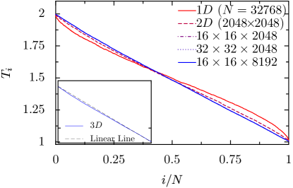
Figure 3: Plot of temperature profiles for a $1D$ system, a $N\times N$ $2D$ system and a $W\times W\times N$ $3D$ system with different aspect ratios $r=W/N$. Temperature profiles for the three aspect ratios overlap with each other. The inset shows that the $3D$ temperature profile is concave upward everywhere.

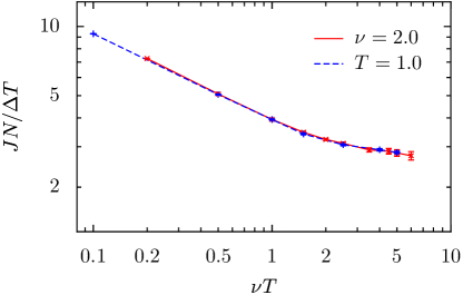
Figure 4: Demonstration of scaling property (4) for $32\times 32\times 128$ system with $\Delta T=0.1$. Thermal conductivities decrease as increasing temperature $T$ or nonlinearity $\nu$. This temperature dependence of $\kappa$ explains the slightly concave curve in temperature profiles in $3D$ (see Fig.(3)).

References

- (1) F. Bonetto, J.L. Lebowitz, and L. Rey-Bellet, in Mathematical Physics 2000, edited by A. Fokas et. al. (Imperial College Press, London, 2000), p. 128.
- (2) J. M. Ziman, Principles of the Theory of Solids,(Cambridge University Press, Cambridge, 1972).
- (3) A. Dhar, Adv. Phys. 57, 457 (2008).
- (4) S. Lepri, R. Livi, and A. Politi, Phys. Rep. 377, 1 (2003).
- (5) S. Lepri, R. Livi and A. Politi, Euro. phys. Lett. 43, 271 (1998).
- (6) O. Narayan and S. Ramaswamy, Phys. Rev. Lett. 89, 200601 (2002).
- (7) G. Basile, C. Bernardin, S. Olla, Phys. Rev. Lett. 96, 204303 (2006).
- (8) A. Lippi and R. Livi, J. Stat. Phys. 100, 1147 (2000).
- (9) P. Grassberger and L. Yang, cond-mat/0204247.
- (10) C. W. Chang et al , Phys. Rev. Lett. 101, 075903 (2008).
- (11) D.L. Nika et al , Appl. Phys. Lett. 94, 203103 (2009).
- (12) A. Chaudhuri et al , arXiv:0902.3350 (2009).
- (13) M. P. Allen and D. L. Tildesley, Computer Simulations of Liquids (Clarendon, Oxford, 1987).
- (14) T. Mai, A. Dhar and O. Narayan, Phys. Rev. Lett. 98, 184301 (2007).
- (15) S Lepri, C Mejia-Monasterio and A Politi, J. Phys. A 42, 025001 (2009).
- (16) A. Dhar and J. L. Lebowitz, Phys. Rev. Lett. 100, 134301 (2008).
- (17) H. Shiba and N. Ito, J. Phys. Soc. Jpn. 77, 054006 (2008).
- (18) T. S. Tighe, J. M. Worlock, M. L. Roukes, Appl. Phys. Lett. 70, 2687 (1997).
- (19) K. Schwab, E. A. Henriksen, J. M. Worlock and M. L. Roukes, Nature 404, 974 (2000).
- (20) D. Li et al , Appl. Phys. Lett. 83, 2934 (2003).