Shell Structure of Confined Charges at Strong Coupling

Abstract

A theoretical description of shell structure for charged particles in a harmonic trap is explored at strong coupling conditions of $\Gamma=50$ and $100$. The theory is based on an extension of the hypernetted chain approximation to confined systems plus a phenomenological representation of associated bridge functions. Predictions are compared to corresponding Monte Carlo simulations and quantitative agreement for the radial density profile is obtained.

Systems of harmonically trapped charged particles exhibit a shell structure in their radial density profile. Recent studies Pohl2004 ; Arp ; Ludwig2005 ; bonitz2006 ; Golubnychiy2006 ; Baumgartner , both experimental and molecular dynamics simulation, indicate the localization of the charges on the surfaces of concentric spheres with a crystal-like ordering on each surface depending on the particle number $N$. These are effectively the zero temperature ground state for the system or energetically close excited states. An accurate and instructive theoretical description of these spherical crystals has been given recently using shell models Baumgartner ; Kraeft06 ; Cioslowski08 . A complementary theoretical description of the fluid phase at finite temperatures has now been given as well Wrighton09 , showing a closely related ”blurred” shell structure that sharpens at stronger Coulomb coupling $\Gamma\equiv q^{2}/r_{0}k_{B}T$ ($q$ is the charge, $r_{0}$ is the ion sphere radius in terms of the average trap density). This fluid phase theory demonstrates that correlations play the dominant role in the formation of shell structure. An extension of the hypernetted chain approximation (HNC) for bulk fluids to the localized charges of a trap was shown to provide all of the qualitative features of shell structure (e.g., number and location of density peaks, shell populations) for the Coulomb coupling constant $\Gamma\geq 10$ . However, comparison with Monte Carlo (MC) simulation results at selected conditions showed significant errors in the HNC amplitudes and widths of the shells ($20-40\%$). An adjusted HNC (AHNC) was proposed to correct these deficiencies, using a phenomenological representation of the neglected ”bridge functions”. Excellent agreement with MC results was obtained in this way for $\Gamma=20,N=25,100$ and $\Gamma=40,N=300$. The objective here is to report further exploration of the AHNC at the stronger coupling values $\Gamma=50$ and $100$, and to note some interesting similarities to the crystal shell structure.

The origin of the AHNC theory for confined systems is summarized briefly first. Consider a system of $N$ classical charges in an external potential. The Hamiltonian for this system is

$$H=H_{0}+\sum_{i=1}^{N}V_{0}(\mathbf{r}_{i}),\hskip 18.06749ptH_{0}=\sum_{i=1}^{N}\frac{1}{2}mv_{i}^{2}+\frac{1}{2}\sum_{i\neq j=1}^{N}V(r_{ij})$$ (1)

where $\vec{r}_{i}$ and $\vec{v}_{i}$ are the position and velocity of charge $i$. The external potential seen by each  particle is denoted by $V_{0}(r)$, and the interaction between the pair $i,j$ is $V(r_{ij})$ (application here will be limited to Coulomb interactions but the discussion is more general). The external potential induces a non-uniform equilibrium density $n(\mathbf{r})$. It follows from density functional theory that $n(\mathbf{r})$ obeys the equation Evans

$$\ln\frac{n(\mathbf{r})\lambda^{3}}{z}=-\beta V_{0}\left(\mathbf{r}\right)-\beta\frac{\delta F_{ex}\left(\beta\mid n\right)}{\delta n\left(r\right)},$$ (2)

where $z=e^{\beta\mu}$, $\mu$ is the chemical potential, and $\lambda=\left(h^{2}\beta/2\pi m\right)^{1/2}$ is the thermal wavelength. The excess free energy $F_{ex}\left(\beta\mid n\right)$ is a universal functional of the density for the Hamiltonian $H_{0}$, independent of the applied external potential $V_{0}$, and describes all correlations among the particles. The solutions to (2) are such that there is a unique equilibrium density $n(\mathbf{r})$ for each $V_{0}(\mathbf{r})$, using the same $F_{ex}\left(\beta\mid n\right)$. A special case is the uniform density of a one component plasma (OCP), resulting from the $V_{0}\left(\mathbf{r}\right)$ for a uniform neutralizing background. The quite different non-uniform density of interest here results from the harmonic trap $V_{0}\left(\mathbf{r}\right)=m\omega^{2}r^{2}/2$. (The spherical symmetry of $V_{0}$ in both cases yields a spherically symmetric density profile in the fluid phase; the broken symmetry crystal profile is not considered here).

This observation that the OCP and trap densities are determined from the same excess free energy functional opens the possibility of describing correlations for the trap in terms of those of the OCP. This is done in reference Wrighton09 with the result

$$\ln\frac{n(r)\lambda^{3}}{z}=-\beta\frac{1}{2}m\omega^{2}r^{2}+\beta\int d\vec{r}^{\prime}\ n(r^{\prime})c_{\mathrm{OCP}}\left(\vec{r}-\vec{r}^{\prime}|;\Gamma\right)+B_{\mathrm{T}}(r|n)$$ (3)

where $c_{\mathrm{OCP}}$ is the direct correlation function of a one-component plasma, and $B_{\mathrm{T}}(r|n)$ is the “bridge function” for the trapping potential. The Ornstein-Zernicke equation relates $c_{\mathrm{OCP}}$ to the pair distribution function for the OCP, $g_{\mathrm{OCP}}$. A similar analysis gives an equation for $g_{\mathrm{OCP}}$

$$\ln g_{\mathrm{OCP}}(r)=-\beta q^{2}r^{-1}+\beta\int d\vec{r}^{\prime}\ \left[g_{\mathrm{OCP}}(r^{\prime})-1\right]c_{\mathrm{OCP}}\left(|\vec{r}-\vec{r}^{\prime}|;\Gamma\right)+B_{\mathrm{OCP}}(r|g_{\mathrm{OCP}}).$$ (4)

These two equations provide a formally exact description of the charged particle system from which approximations can be made. In particular, the HNC approximation for both the OCP and the trap density is defined by the neglect of both bridge functions in these equations. The trap density is then determined entirely in terms of correlations for the OCP.

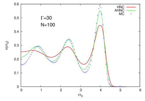
Figure 1: Comparison of HNC and adjusted HNC (AHNC) to Monte Carlo (MC) results. Conditions are $\Gamma=30$ and $N=100$.

The HNC density profile is very accurate at weak to moderate coupling, $\Gamma<10$, but has significant quantitative errors as the shell structure develops at larger values of the coupling. This is illustrated in Figure 1 for $\Gamma=30,N=100$. It was proposed in reference Wrighton09 to improve the HNC by a phenomenological representation of the bridge functions in the form

$$B(r|n)\rightarrow\lambda(\Gamma)\beta V_{0}(r),$$ (5)

where $V_{0}$ is the harmonic potential for $B_{\mathrm{T}}$ or Coulomb potential for $B_{\mathrm{OCP}}$. Also $\lambda(\Gamma)$ is chosen to interpolate between $\lambda(0)=0$ and some constant $\lambda(\infty)$. This approach was first introduced by Ng Ng for the OCP pair distribution. Subsequently, Rosenfeld and Ashcroft have defined related ”modified” HNC approximations using the bridge function as a fitting function Rosenfeld78 . The advantage of the form (5) is that the effect of the bridge functions is to simply ”renormalize” the external potential in both eqs. (3) and (4), so that the original HNC approximation is regained except with an effective coupling constant $\Gamma^{\prime}$ defined by

$$\Gamma^{\prime}=\left[1+\lambda(\Gamma)\right]\Gamma$$ (6)

In the original work of Ng, he obtained agreement with the Monte Carlo data for $g_{\mathrm{OCP}}$ to within a few percent using $\lambda(\infty)=0.6$. That same value for $\lambda(\infty)$ has been used in reference Wrighton09 and in the results presented here.

The improvement gained from this AHNC is also shown in Figure 1. All three curves agree regarding the number of peaks and the location of the peaks. Also, there is quantitative agreement regarding the number of charges in each shell (not shown). However, the HNC and AHNC results give very different heights and widths of the peaks themselves. Comparison to the MC results makes it clear that the bridge function effects are important at this value of the coupling constant. Similar improvement has been illustrated for $\Gamma=20$ and $40$ for several values of $N$ Wrighton09 .

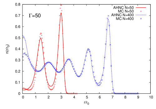
Figure 2: Comparison of density profile for AHNC and MC, for $\Gamma=50$, $N=50$ and $400$

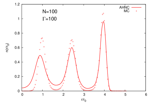
Figure 3: Comparison of density profile for AHNC and MC results for $\Gamma=100$ and $N=100$.

It remains to explore how well this approach extends to still larger values of $\Gamma$, motivated by its possible utility to study freezing into a spherical crystal.  As a first step in that direction results are presented and discussed here for $\Gamma=50,100$. Figure (2) shows the density profile at $\Gamma=50$ for two quite different particle numbers $N=50$ and $N=400$. For small enough particle number, $N\lesssim 20$, there is only one shell of finite radius near the point at which the density vanishes Ludwig2005 . The latter is fixed by the condition that the Coulomb force on a test charge balances that of the trap, i.e. $r_{max}=N^{1/3}$. A second shell is present at $N=50$, while three additional shells are observed for $N=400$ (as well as a population at the origin bonitz2006 ). The agreement between MC and AHNC is seen to be quite good in both cases except at very small $r$ for which the both HNC and AHNC fail even at moderate coupling.

The discrepancies in amplitudes increase somewhat at very strong coupling. This is illustrated in Figure (3) showing the comparison of MC and AHNC results for $\Gamma=100,N=100$. The error in peak height grows from about $10\%$ for  the outer shell to about $30\%$ for the inner shell. Still the overall agreement remains quite good. To explore the conditions for freezing into spherical crystals, even stronger coupling conditions, $\Gamma\sim 200$ are expected to be relevant. However, several important features of the crystal ground state are already evident from the fluid phase AHNC results at the coupling conditions studied. Figure (4) shows a comparison of shell populations from ground state annealed MD simulations Arp with those from AHNC. The latter have been computed for $20\leq\Gamma\leq 100$, showing a very weak dependence on coupling strength. This is somewhat unexpected since the amplitudes and widths of the shells are quite sensitive to $\Gamma$. The shell populations and appearance of shells is clearly quite similar in the fluid and crystal phases. Figure (5) shows a corresponding comparison of shell locations as a function of $N$. Again the results are remarkably close for both fluid and crystal phases.

The results for the ground state shown on Figures (4) and (5) can be understood theoretically on the basis of a shell model. This represents the density as a sum of delta functions for particle positions on shells of radii $r_{\nu}$ and occupancy $n_{\nu}$

$$n(\mathbf{r})=\sum_{\nu}n_{\nu}\frac{1}{4\pi r_{\nu}^{2}}\delta\left(r\mathbf{-}r_{\nu}\right),\hskip 18.06749pt\sum_{\nu}n_{\nu}=N.$$ (7)

The values of $n_{\nu},r_{\nu}$ are determined by minimizing the total energy Baumgartner ; Kraeft06 . A very accurate representation of the energy for this purpose is constructed on the basis of solutions to the Thomson problem Thomson for ground state configurations of Coulomb charges on a single sphere Cioslowski08 . The intrashell energy is chosen as the known Thomson energy for each $n_{\nu},r_{\nu}$, while the intershell energy is taken as the monopole interactions for charges at the corresponding Thomson positions for each shell. In this way the crystal energy, shell populations, and locations are given very accurately. This opens the possibility to test free energies associated with (3) and (4) for broken rotational invariance using parameterized densities similar to the shell model (e.g., Gaussians centered at the Thomson positions) to identify a freezing transition.

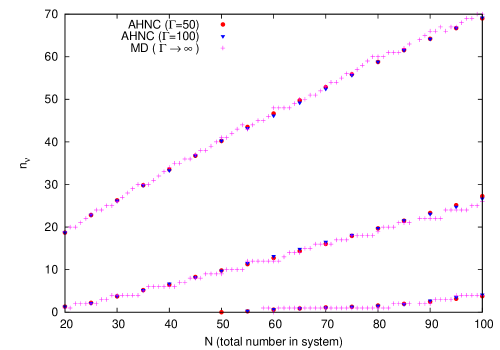
Figure 4: Comparison of shell populations from AHNC and MD as a function of particle number $N$.

Figure 5: Comparison of shell radii from AHNC and MD as a function of particle number $N$.

This work is supported by the Deutsche Forschungsgemeinschaft via SFB-TR 24, and by the NSF/DOE Partnership in Basic Plasma Science and Engineering under the Department of Energy award DE-FG02-07ER54946.

References

- (1) T. Pohl, T. Pattard, and J.M. Rost, Phys. Rev. Lett. 92, 155003 (2004).
- (2) O. Arp, D. Block, A. Piel, and A. Melzer, Phys. Rev. Lett. 93, 165004 (2004); O. Arp, D. Block, M. Bonitz, H. Fehske, V. Golubnychiy, S. Kosse, P. Ludwig, A. Melzer, and A. Piel, J. Phys. Conf. Series 11, 234 (2005).
- (3) P. Ludwig, S. Kosse, and M. Bonitz, Phys. Rev. E 71, 046403 (2005).
- (4) M. Bonitz, D. Block, O. Arp, V. Golubnychiy, H. Baumgartner, P. Ludwig, A. Piel, and A. Filinov, Phys. Rev. Lett. 96, 075001 (2006).
- (5) V. Golubnychiy, H. Baumgartner, M. Bonitz, A. Filinov, and H. Fehske, J. Phys. A: Math. Gen. 39, 4527 (2006).
- (6) H. Baumgartner, H. Kählert, V. Golubnychiy, C. Henning, S. Käding, A. Melzer, and M. Bonitz, Contrib. Plasma Phys. 47, 281 (2007); H. Baumgartner, D. Asmus, V. Golubnychiy, P. Ludwig, H. Kählert, and M. Bonitz, New Journal of Physics 10, 093019 (2008).
- (7) W. D. Kraeft and M. Bonitz, J. Phys. Conf. Ser. 35, 94 (2006).
- (8) J. Cioslowski and E. Grzebielucha, Phys. Rev E 78, 026416 (2008).
- (9) J. Wrighton, J. W. Dufty, H. Kählert, and M. Bonitz. “Theoretical Description of Coulomb Balls – Fluid Phase”, arXiv:0909.0775.
- (10) R. Evans, in Fundamentals of Inhomogeneous Fluids, edited by D. Henderson (Marcel Dekker, NY, 1992).
- (11) K. C. Ng, J. Chem. Phys. 61, 2680-2689 (1974).
- (12) Y. Rosenfeld and N. W. Ashcroft, Phys. Rev. A 20, 1208 (1979).
- (13) J. P. Schiffer, Phys. Rev. Lett. 88, 205003 (2002).
- (14) J. J. Thomson, Philos. Mag. 7, 237 (1904).