Analysis of a mathematical model of
ischemic cutaneous wounds

Abstract

Chronic wounds represent a major public health problem affecting 6.5 million people in the United States. Ischemia represents a serious complicating factor in wound healing. In this paper we analyze a recently developed mathematical model of ischemic dermal wounds. The model consists of a coupled system of partial differential equations in the partially healed region, with the wound boundary as a free boundary. The extracellular matrix (ECM) is assumed to be viscoelastic, and the free boundary moves with the velocity of the ECM at the boundary of the open wound. The model equations involve the concentrations of oxygen, cytokines, and the densities of several types of cells. The ischemic level is represented by a parameter which appears in the boundary conditions, $0\leq\gamma<1$; $\gamma$ near 1 corresponds to extreme ischemia and $\gamma=0$ corresponds to normal non-ischemic conditions. We establish global existence and uniqueness of the free boundary problem and study the dependence of the free boundary on $\gamma$.

1 Introduction

Wound healing represents the outcome of a large number of interrelated biological events that are orchestrated over a temporal sequence in response to injury and its microenvironment. The process involves interactions among different soluble chemical mediators, different types of cells, and the extracellular matrix (ECM). Among the various factors that affect the healing of a wound, the tissue oxygen level is a key determinant [11, 26]. Although hypoxia is generally recognized as a physiological cue to induce angiogenesis [4, 25, 21, 14], severe hypoxia cannot sustain the growth of functional blood vessels [12, 1, 10, 18, 23].

There have been several mathematical models of wound healing which incorporated the effect of angiogenesis [20, 19, 3, 24]. Mathematical models of angiogenic networks, such as through the induction of vascular networks by vascular endothelial growth factors (VEGFs) [5, 6], were developed by McDougall and coworkers [16, 27], based in part on the work of Anderson and Chaplain [2], in connection with chemotherapeutic strategies. The role of oxygen in wound healing was explicitly incorporated in the works of Byrne et al. [3] and Schugart et al. [24]. In particular, it was demonstrated in [24] that enhanced healing can be achieved by moderate hyperoxic treatments. In [22], the impairment of dermal wound healing due to ischemic conditions was addressed in a pre-clinical experimental model. In a more recent work [28], Xue, Friedman and Sen developed a mathematical model of ischemic dermal wound-healing. The model consists of a system of PDEs in the partially healed region which is modeled as a viscoelastic medium with a free boundary surrounding the open wound. Simulations of the model were shown to be in agreement with the experimental results in [22].

In this paper we study the model in [28] by mathematical analysis. In particular we prove that the free boundary problem developed in that model has a unique global solution, and that the open wound does not close under extreme ischemic conditions. We also show, by simulations, that non-ischemic wounds do heal. In Section 2 we formulate the mathematical model for a radially symmetric geometry as in [28]. The ischemic level is determined by a parameter $\gamma$, $0\leq\gamma\leq 1$; $\gamma$ near 1 corresponds to extreme ischemia and $\gamma=0$ corresponds to normal non-ischemic conditions. In Section 3 we show that the free boundary is monotone decreasing, and in Section 4 we derive a priori estimates. In Section 5 we transform the free boundary problem into a problem in a fixed domain; this is a convenient form for proving, in Section 6, local existence and uniqueness of a solution. The extension of the solution to all $t>0$ is also established in Section 6, by using the a priori estimates derived in Section 4. In Section 7 we consider the case of extreme ischemia (namely, $\gamma$ near 1) and prove that the wound’s boundary stops decreasing after some finite time. In Section 8 we establish some properties of the solution for wounds that do not heal. Section 9 simulates the radius of the wound when the parameter of the system are chosen, as in [28], based on biological literature. The simulations suggest the following conjecture: there exists a parameter $\gamma^{\ast}$ such that wounds heal if $0\leq\gamma<\gamma^{\ast}$ and do not heal if $\gamma^{\ast}<\gamma\leq 1$.

2 The mathematical model

It is assumed that the dermal tissue is in a circular domain $\{(r,\theta;\;r\leq L)\}$ and the open wound at time $t$ is a disc $\{(r,\theta;\;r<R(t))\}$ with initial radius $R(0)<L$. The partially healed tissue is the annulus $\Omega(t)=\{(r,\theta;\;R(t)\leq r\leq L)\}$. We introduce the following variables:

• Chemicals:

  • $w(r,t)$: concentration of tissue oxygen

  • $e(r,t)$: concentration of Vascular Endothelial Growth Factor (VEGF)

  • $p(r,t)$: concentration of Platelet Derived Growth Factor (PDGF)

• Cells, blood vessels and matrix

  • $m(r,t)$: density of macrophages

  • $f(r,t)$: density of fibroblasts

  • $n(r,t)$: density of capillary tips

  • $b(r,t)$: density of capillary sprouts

  • $\rho(r,t)$: density of the ECM

  • $v(r,t)$: velocity of the ECM

In homeostasis $w=w_{0}$, $m=m_{0}$, $f=f_{0}$, $b=b_{0}$ and $\rho=\rho_{0}$. In the remainder of this paper these variables have already been scaled so that $w_{0}=m_{0}=\rho_{0}=b_{0}=\rho_{0}=1$.

The continuity equation for the matrix density $\rho$ is

$$\dfrac{\partial\rho}{\partial t}+\nabla\cdot(\rho\mathbf{v})=G_{\rho}(f,w,p),$$

where $G_{\rho}(f,w,\rho)$ is a growth and decay term of the ECM due to collagen secretion by fibroblasts and degradation by matrix metalloproteinases (MMPs). The specific form of $G_{\rho}$ incorporates the fact that collagen production and maturation require the availability of oxygen [13, 17, 11, 26],

$$G_{\rho}=\frac{k_{\rho}w}{w+K_{w\rho}}f(1-\frac{\rho}{\rho_{m}})-\lambda_{\rho}\rho,$$

where $\rho_{m}$ is the maximum matrix volume fraction permitted in the partially healed region, $\rho_{m}>1$.

The partially healed tissue is modeled as a quasi-static upper convected Maxwell fluid with velocity $\mathbf{v}$, deviatoric stress tensor given by $\tau=\eta(\nabla\mathbf{v}+\nabla\mathbf{v}^{T})$, where $\eta$ is the shear viscosity, and pressure $P$. The pressure $P$ is generally a function of the matrix density $\rho$, and is assumed to have the form

$$P(\rho)=\left\{\begin{aligned} &\beta(\rho-1),&&\rho\geq 1\\ &0,&&\rho<1.\end{aligned}\right.$$ (2.1)

The total stress $\sigma=\tau-PI$ appears only in the boundary conditions. By further assuming radially symmetric flow, i.e., $\mathbf{v}=v(r,t)\mathbf{e}_{r}$, the continuity equation becomes

$$\dfrac{\partial\rho}{\partial t}+\frac{1}{r}\dfrac{\partial}{\partial r}\big{(}r\rho v\big{)}=\frac{k_{\rho}w}{w+K_{w\rho}}f(1-\frac{\rho}{\rho_{m}})-\lambda_{\rho}\rho,\quad R(t)<r<L,$$ (2.2)

and the non-dimensionalized momentum equation for the ECM becomes (see [28], supporting information)

$$\frac{1}{r}\dfrac{\partial}{\partial r}\left(r\dfrac{\partial v}{\partial r}\right)-\frac{v}{r^{2}}=\dfrac{\partial P(\rho)}{\partial r},\quad R(t)<r<L.$$ (2.3)

To simplify the analysis and simulations we wish to have a PDE system in which all variables are radially symmetric. In order to implement ischemic conditions in radially symmetric form we assume that small arcs of length $\delta$ are cut off from the healthy tissue at $r=L$ and that the distance between two adjacent $\delta$ arcs is $\varepsilon$. If $\delta,\;\varepsilon\to 0$ in such a way that $\varepsilon\sim e^{-c/\delta}$ where $c$ is a positive constant, then, for any diffusion process with boundary conditions

$$\dfrac{\partial u}{\partial r}=0\;\; \mbox{on the}\;\delta\mbox{-arcs},$$

$$u=g\;\; \mbox{on the remaining arcs},$$

the limiting “homogenized” boundary condition is [8]

$$(1-\gamma)(u-g)+\gamma\dfrac{\partial u}{\partial r}=0\quad\text{on}\;\;r=L$$

for some constant $\gamma\in[0,1]$ which depends only on $c$; $\gamma=0$ corresponds to healthy tissue (i.e., no excision of $\delta$-arcs) and $\gamma$ near 1 corresponds to extreme ischemia.

The equations for the concentrations of oxygen, PDGF and VEGF are:

$$\frac{\partial w}{\partial t}+\frac{1}{r}\dfrac{\partial}{\partial r}\big{(}rwv\big{)}=\frac{1}{r}\frac{\partial}{\partial r}\left(rD_{w}\dfrac{\partial w}{\partial r}\right)$$ (2.4)

$$\hskip 56.9055pt+k_{w}b\big{(}(1-\gamma)w_{b}-w\big{)}-\left[\big{(}\lambda_{wf}f+\lambda_{wm}m\big{)}\left(1+\dfrac{\lambda_{ww}p}{1+p}\right)+\lambda_{wm}\right]w,$$

$$\frac{\partial p}{\partial t}+\frac{1}{r}\dfrac{\partial}{\partial r}\big{(}rpv\big{)}=\frac{1}{r}\frac{\partial}{\partial r}\left(rD_{p}\dfrac{\partial p}{\partial r}\right)+k_{p}mG_{p}(w)-\dfrac{\lambda_{pf}fp}{1+p}-\lambda_{p}p,$$ (2.5)

$$\frac{\partial e}{\partial t}+\frac{1}{r}\dfrac{\partial}{\partial r}\big{(}rev\big{)}=\frac{1}{r}\frac{\partial}{\partial r}\left(rD_{e}\dfrac{\partial e}{\partial r}\right)+k_{e}mG_{e}(w)-(\lambda_{en}n+\lambda_{eb}b+\lambda_{e})e,$$ (2.6)

The equations for macrophages, fibroblasts, capillary tips and capillary sprouts include diffusion, generation and death of cells, and chemotactic migration of cells:

$$\frac{\partial m}{\partial t}+\frac{1}{r}\dfrac{\partial}{\partial r}\big{(}rmv\big{)}=\frac{1}{r}\frac{\partial}{\partial r}\left(rD_{m}\dfrac{\partial m}{\partial r}\right)-\frac{1}{r}\frac{\partial}{\partial r}\left(r\frac{\chi_{m}\rho mH(1-m/m_{m}){\partial p}/{\partial r}}{\sqrt{1+k_{sg}\left|{\partial p}/{\partial r}\right|^{2}}}\right)$$ (2.7)

$$\hskip 142.26378pt+\frac{k_{m}bp}{1+p}-\lambda_{m}m\left(1+\lambda_{d}D(w)\right),$$

$$\frac{\partial f}{\partial t}+\frac{1}{r}\dfrac{\partial}{\partial r}\big{(}rfv\big{)}=\frac{1}{r}\frac{\partial}{\partial r}\left(rD_{f}\dfrac{\partial f}{\partial r}\right)-\frac{1}{r}\frac{\partial}{\partial r}\left(r\frac{\chi_{f}\rho fH(1-f/f_{m}){\partial p}/{\partial r}}{\sqrt{1+k_{sg}\left|{\partial p}/{\partial r}\right|^{2}}}\right)$$ (2.8)

$$\hskip 142.26378pt+k_{f}G_{f}(w)f\left(1-\frac{f}{f_{m}}\right)-\lambda_{f}f(1+\lambda_{d}D(w)),$$

$$\frac{\partial n}{\partial t}+\frac{1}{r}\dfrac{\partial}{\partial r}\big{(}rnv\big{)}=\frac{1}{r}\frac{\partial}{\partial r}\left(rD_{n}\dfrac{\partial n}{\partial r}\right)-\frac{1}{r}\frac{\partial}{\partial r}\left(r\frac{\chi_{n}\rho nH(1-n/n_{m}){\partial e}/{\partial r}}{\sqrt{1+k_{sg}\left|{\partial e}/{\partial r}\right|^{2}}}\right)$$ (2.9)

$$\hskip 113.81102pt+(k_{nb}b+k_{n}n)\frac{e}{1+e}-(\lambda_{nb}b+\lambda_{nn}n)n,$$

$$\frac{\partial b}{\partial t}+\frac{1}{r}\dfrac{\partial}{\partial r}\big{(}rbv\big{)}=\frac{1}{r}\frac{\partial}{\partial r}\left(rD_{b}\dfrac{\partial b}{\partial r}\right)+\frac{1}{r}\frac{\partial}{\partial r}\left(r\frac{AD_{n}b{\partial n}/{\partial r}}{\sqrt{1+k_{sg}\left|{\partial n}/{\partial r}\right|^{2}}}\right)$$ (2.10)

$$\hskip 113.81102pt-\frac{1}{r}\frac{\partial}{\partial r}\left(r\frac{A\chi_{n}b\rho nH(1-n/n_{m}){\partial e}/{\partial r}}{\sqrt{1+k_{sg}\left|{\partial e}/{\partial r}\right|^{2}}}\right)$$

$$\hskip 113.81102pt+k_{b}G_{b}(w)b(1-b)+G_{b}(w)(\lambda_{nb}b+\lambda_{nn}n)n.$$

where the two terms with $A$ (in (2.10)) represent the fact that sprouts follow tips, and the oxygen-dependent functions $G$’s and $D$ are given by

$$G_{p}(w)=\left\{\begin{aligned} &3w,&&0\leq w<0.5\\ &2-w,&&0.5\leq w<1\\ &\frac{1}{3}w+\frac{2}{3},&&1\leq w<4\\ &2,&&w\geq 4\end{aligned}\right.,\qquad G_{e}(w)=\left\{\begin{aligned} &2w,&&0\leq w<0.5,\\ &2-2w,&&0.5\leq w<1,\\ &\frac{1}{3}w-\frac{1}{3},&&1\leq w<4,\\ &1,&&w\geq 4\end{aligned}\right.,$$

$$G_{f}(w)=\dfrac{(K_{wf}+1)w}{K_{wf}+w},\quad G_{b}=\dfrac{(K_{w\rho}+1)w}{K_{w\rho}+w},\quad D(w)=1-H(5w-1)H(1-w/3).$$

Here $H$ is an approximated Heaviside function

$$H(u)=\left\{\begin{aligned} &\frac{u^{6}}{10^{-6}+u^{6}},&&u\geq 0\\ &0,&&u<0.\end{aligned}\right.$$

Note that in Equation $($2.4$)$ the supply of oxygen from the vasculature is reduced to $k_{w}b((1-\gamma)w_{b}-w)$ due to the ischemic condition. The functions $G_{p}(w)$ and $G_{e}(w)$ are constructed to reflect the biological effect of oxygenation: moderate hypoxia and hyperoxia increase the production of PDGF and VEGF compared to normoxia. Equations $($2.7$)$ - $($2.9$)$ include chemotaxis flux terms that describe the chemotactic movement of macrophages, fibroblasts and capillary tips. The two terms with $A$ in Equation $($2.10$)$ represent the fact that capillary sprouts are dragged along capillary tips. Although the forms of the $G$ functions and $D$ function are suggested by biological experiments, our mathematical analysis will not depend on the special form of these functions.

The free boundary $r=R(t)$ is moving with velocity $v$:

$$\dot{R}(t)=v(R(t),t).$$ (2.11)

The boundary conditions at $r=L$ are

$$v=0,$$ (2.12)

$$(1-\gamma)(w-1)+\gamma L\dfrac{\partial w}{\partial r}=0,$$ (2.13)

$$(1-\gamma)p+\gamma L\dfrac{\partial p}{\partial r}=0,\quad(1-\gamma)e+\gamma L\dfrac{\partial e}{\partial r}=0,$$ (2.14)

$$(1-\gamma)m+\gamma L\left(\dfrac{\partial m}{\partial r}-\dfrac{\chi_{m}}{D_{m}}\frac{\rho mH(1-m/m_{m}){\partial p}/{\partial r}}{\sqrt{1+k_{sg}\left|{\partial p}/{\partial r}\right|^{2}}}\right)=0,$$ (2.15)

$$(1-\gamma)(f-1)+\gamma L\left(\dfrac{\partial f}{\partial r}-\dfrac{\chi_{f}}{D_{f}}\frac{\rho fH(1-f/f_{m}){\partial p}/{\partial r}}{\sqrt{1+k_{sg}\left|{\partial p}/{\partial r}\right|^{2}}}\right)=0,$$ (2.16)

$$(1-\gamma)n+\gamma L\left(\dfrac{\partial n}{\partial r}-\dfrac{\chi_{n}}{D_{n}}\frac{\rho nH(1-n/n_{m}){\partial e}/{\partial r}}{\sqrt{1+k_{sg}\left|{\partial e}/{\partial r}\right|^{2}}}\right)=0,$$ (2.17)

$$(1-\gamma)(b-1)+\gamma L\left(\dfrac{\partial b}{\partial r}+\frac{AD_{n}b{\partial n}/{\partial r}}{\sqrt{1+k_{sg}\left|{\partial n}/{\partial r}\right|^{2}}}-\frac{A\chi_{n}b\rho nH(1-n/n_{m}){\partial e}/{\partial r}}{\sqrt{1+k_{sg}\left|{\partial e}/{\partial r}\right|^{2}}}\right)=0,$$ (2.18)

and the boundary conditions at $r=R(t)$ are

$$\dfrac{\partial v}{\partial r}=P,$$ (2.19)

$$\dfrac{\partial w}{\partial r}=\dfrac{\partial e}{\partial r}=\dfrac{\partial n}{\partial r}=\dfrac{\partial b}{\partial r}=0,$$ (2.20)

$$-\dfrac{\partial p}{\partial r}=\frac{k_{pb}R(t)}{D_{p}R_{0}},$$ (2.21)

$$-D_{m}\dfrac{\partial m}{\partial r}+\chi_{m}\frac{\rho mH(1-m/m_{m}){\partial p}/{\partial r}}{\sqrt{1+k_{sg}\left|{\partial p}/{\partial r}\right|^{2}}}=0,$$ (2.22)

$$-D_{f}\dfrac{\partial f}{\partial r}+\chi_{f}\frac{\rho fH(1-f/f_{m}){\partial p}/{\partial r}}{\sqrt{1+k_{sg}\left|{\partial p}/{\partial r}\right|^{2}}}=0,$$ (2.23)

Equation $($2.21$)$ represents the fact that secretion of platelets decreases with healing (i.e., as $R(t)$ decreases). The initial conditions for $R_{0}\leq r\leq L$ take the form

$$R(0)=R_{0},\;\;v=0,\;\;\rho=f=1,\;\;w=1,\;\;b=g\left(\frac{r-R_{0}}{\epsilon_{0}}\right),$$ (2.24)

$$e=m=n=0,\;\;p=p_{0}(r),$$

where

$$g(z)=\left\{\begin{aligned} &0,&&\qquad z\leq 0,\\ &\frac{8}{3}z^{2},&&\qquad 0<z\leq\frac{1}{4},\\ &\frac{4}{3}z-\frac{1}{6},&&\qquad\frac{1}{4}\leq z<\frac{3}{4},\\ &1-\frac{8}{3}(1-z)^{2},&&\qquad\frac{3}{4}\leq z\leq 1,\\ &1,&&\qquad z>1.\end{aligned}\right.$$

and $p_{0}(r)$ has three continuous derivatives and satisfies the boundary conditions (2.14) and (2.21), and

$$\left\{\begin{aligned} &p_{0}^{\prime}(r)<0&&\mbox{if}&&R_{0}<r<R_{0}+\varepsilon_{0},\\ &p_{0}(r)=0&&\mbox{if}&&R_{0}+\varepsilon_{0}<r<L\end{aligned}\right.$$ (2.25)

where $0<\varepsilon_{0}<L-R_{0}$.

In a healthy tissue there is no net growth of ECM, i.e., $G_{\rho}(f,w,\rho)=0$ if $f=w=\rho=1$, which means that

$$\lambda_{\rho}=\frac{k_{\rho}}{1+K_{w\rho}}\left(1-\frac{1}{\rho_{m}}\right).$$ (2.26)

Similarly

$$k_{w}=\frac{\lambda_{wf}+\lambda_{wm}}{w_{b}-1},$$ (2.27)

$$k_{f}=\dfrac{\lambda_{f}}{1-1/f_{m}}.$$ (2.28)

3 ${R}(t)$ is monotonically decreasing

Set

$$Q(t)=\int_{R(t)}^{L}yP(y,t)dy,$$ (3.1)

where $P(r,t)=P(\rho(r,t))$.

Theorem 3.1.

For any solution of (2.2)-(2.28) there holds:

$$\dot{R}(t)\leq 0;\;\;\dot{R}(t)<0\;\mbox{ if and only if }\;\;Q(t)>0;$$ (3.2)

$$R(0)e^{-\frac{2}{L^{2}}\int_{0}^{t}Q(\tau)d\tau}\leq R(t)\leq R(0)e^{-\frac{1}{L^{2}}\int_{0}^{t}Q(\tau)d\tau}.$$ (3.3)

Proof. Equation (2.3) can be rewritten as

$$v_{rr}+\frac{v_{r}}{r}-\frac{v}{r^{2}}=v_{rr}+\left(\frac{v}{r}\right)_{r}=P_{r}.$$

Integrating over $[R(t),r]$, we obtain

$$v_{r}(r,t)-v_{r}(R(t))+\frac{v(r,t)}{r}-\frac{v(R(t))}{R(t)}=P(r,t)-P(R(t),t).$$

From (2.11) and (2.19) we obtain

$$v_{r}(r,t)+\frac{v(r,t)}{r}-\frac{\dot{R}(t)}{R(t)}=P(r,t),$$

hence

$$(rv)_{r}-r\frac{\dot{R}(t)}{R(t)}=rP(r,t).$$ (3.4)

Integrating this equation over $[r,L]$ and using (2.12), we obtain

$$-rv(r,t)-\frac{L^{2}-r^{2}}{2}\frac{\dot{R}(t)}{R(t)}=\int_{r}^{L}yP(y,t)dy.$$ (3.5)

In particular, at $r=R(t)$,

$$-R(t)\dot{R}(t)-\frac{L^{2}-R(t)^{2}}{2}\frac{\dot{R}(t)}{R(t)}=\int_{R(t)}^{L}yP(y,t)dy,$$

or

$$\frac{\dot{R}(t)}{R(t)}=-\frac{2}{L^{2}+R(t)^{2}}Q(t).$$ (3.6)

The assertion (3.2) now follows immediately from (3.6). From (3.6) we also obtain

$$-\frac{2}{L^{2}}Q(t)\leq\frac{\dot{R}(t)}{R(t)}\leq-\frac{1}{L^{2}}Q(t),$$ (3.7)

from which we deduce the estimate (3.3).        

If we substitute $\dot{R}/R$ from (3.6) into (3.4) we obtain, after dividing by $r$,

$$\frac{(rv)_{r}}{r}=P(r,t)-\frac{2}{L^{2}+R(t)^{2}}Q(t);$$ (3.8)

this equation will be needed in the remainder of this paper. If we substitute $\dot{R}/R$ from (3.6) into (3.5), and divide by $r$, we obtain an expression for $v$,

$$v(r,t)=\frac{1}{r}\left\{\frac{L^{2}-r^{2}}{L^{2}+R(t)^{2}}Q(t)-\int_{r}^{L}yP(y,t)dy\right\}$$

or

$$v(r,t)=\frac{1}{r}\left\{\frac{L^{2}-r^{2}}{L^{2}+R(t)^{2}}\int_{R(t)}^{r}yP(y,t)dy-\frac{r^{2}+R(t)^{2}}{L^{2}+R(t)^{2}}\int_{r}^{L}yP(y,t)dy\right\}$$ (3.9)

Corollary 3.2.

Equation (2.3) for $v$ together with the boundary conditions (2.12), (2.19) and the initial condition $v=0$ can be equivalently replaced by the formula (3.9) .

In the remainder of this paper we shall often work with the representation (3.9) for $v$.

4 A priori estimates

In this section we assume that there exists a classical solution to (2.2) – (2.28) for $0\leq t<T$, and derive a priori estimates which depend on $T$, but remain uniformly bounded for any finite $T$. We set

$$\Omega_{T}=\{(r,\theta,t)\;|\;R(t)<r<L,\;0\leq\theta\leq 2\pi,\;0<t\leq T\}$$

and introduce the following notation:

$C_{r,t}^{2+\alpha,1+\alpha/2}(\bar{\Omega}_{T})$ is the space of functions $u(r,t)$ with $u$, $D^{2}_{r}u$, $D_{t}u$ uniformly Hölder continuous in $\bar{\Omega}_{T}$, with exponents $\alpha$ in $r$ and $\alpha/2$ in t; the norm in this space is defined by

$$\|u\|_{C_{r,t}^{2+\alpha,1+\alpha/2}(\bar{\Omega}_{T})}=\|u\|_{L^{\infty}(\bar{\Omega}_{T})}+\|D^{2}_{r}u\|_{C_{r,t}^{\alpha,\alpha/2}(\bar{\Omega}_{T})}+\|D_{t}u\|_{C_{r,t}^{\alpha,\alpha/2}(\bar{\Omega}_{T})}$$

where

$$\|v\|_{C_{r,t}^{\alpha,\alpha/2}(\bar{\Omega}_{T})}=\|v\|_{L^{\infty}(\Omega_{T})}+\sup_{(r,t),(r^{\prime},t^{\prime}))\in\bar{\Omega}_{T}}\frac{|v(r,t)-v(r^{\prime},t^{\prime})|}{|r-r^{\prime}|^{\alpha}+|t-t^{\prime}|^{\alpha/2}}.$$

Similarly we define the spaces $C_{r,t}^{\alpha,\beta}(\bar{\Omega}_{T})$, $C^{1+\alpha}[0,T]$, etc.

In the remainder of this paper we shall use the following comparison principle [7, 15].

Lemma 4.1.

Let $v_{1}$, $v_{2}$ satisfy

$$\dfrac{\partial v_{1}}{\partial t}-D\Delta v_{1}+g(x,t,v_{1},\nabla v_{1})\geq\dfrac{\partial v_{2}}{\partial t}-D\Delta v_{2}+g(x,t,v_{2},\nabla v_{2})\quad\text{in}\;\;\Omega_{T}.$$ (4.1)

If

$$\mu_{1}\dfrac{\partial}{\partial\nu}(v_{1}-v_{2})+\mu_{2}(v_{1}-v_{2})\geq 0\quad\text{on}\;\;\partial\Omega_{T}\cap\{0<t<T\},$$ (4.2)

$$(v_{1}-v_{2})|_{t=0}\geq 0\quad\text{in}\;\;\Omega_{0}$$

where $\nu$ is the outward normal and $\mu_{1}$, $\mu_{2}$ are nonnegative functions satisfying, at each point, either $\mu_{1}>0$ or $\mu_{1}=0$,$\mu_{2}>0$, then $v_{1}\geq v_{2}$ in $\Omega_{T}$. Furthermore, if strict inequalities hold in both $($4.1$)$ and $($4.2$)$, then $v_{1}>v_{2}$ in $\Omega_{T}$.

Lemma 4.2.

For any solution of $($2.2$)$ – $($2.28$)$,

$$\mbox{the components }w,\;e,\;p,\;m,\;f,\;n,\;b,\;\mbox{ and }\rho\mbox{ are nonnegative functions.}$$ (4.3)

Proof. For any small $\delta>0$, let us add $\delta$ on the right-hand side of each of the equations $($2.4$)$-$($2.10$)$ and each of the boundary conditions $($2.13$)$-$($2.18$)$, $($2.21$)$-$($2.23$)$, replace $0$ by $-\delta$ in $($2.20$)$, and increase the initial data of $b,e,m,n,p$ by $\delta$. We refer to this new system as the “$\delta$-problem” and to its solution as the “$\delta$-solution”. By continuity, each component of the $\delta$-solution is strictly positive in $\Omega_{t_{0}}$ for some $t_{0}>0$. We claim that all the components are strictly positive in $\Omega_{T}$ for all $T>0$. Indeed, otherwise there is a smallest $T$ such that at least one component of the $\delta$-solution, denoted by $z$, vanishes at some point $(\bar{r},T)$. We can then apply the second part of Lemma 4.1 with $v_{1}=z$, $v_{2}=0$ to conclude that $z(\bar{r},T)>0$, which is a contradiction.

The local existence and uniqueness proof given in Sections 4-6 is valid also for the $\delta$-problem. The estimates derived there are uniform in $\delta$ so that, as $\delta\to 0$, the $\delta$-solution converges to the original solution. Hence each component of the original solution is non-negative in a small time interval, say $0<t<t_{\ast}$. We can now repeat the process for $t>t_{\ast}$, and conclude, step-by-step that each component of the solution is non-negative in $\Omega_{T}$ for any $T>0$.        

Lemma 4.3.

If initially $\rho(r,0)<\rho_{m}$ for $R(0)\leq r\leq L$, then,

$$\rho<\rho_{m}\qquad\mbox{in}\;\;\Omega_{T}.$$ (4.4)

Proof. If the assertion (4.4) is not true, then there exists a $t^{\ast}>0$ such that $\rho(r,t)<\rho_{m}$ in $\Omega_{t^{\ast}}$, and $\rho(r^{\ast},t^{\ast})=\rho_{m}$ for some $R(t^{\ast})\leq r^{\ast}\leq L$. Then, along the characteristic curve with velocity $v$, through $(r^{\ast},t^{\ast})$,

$$\left.\frac{D\rho}{Dt}\right|_{(r^{\ast},t^{\ast})}\geq 0,$$ (4.5)

where $D/Dt=\partial/\partial t+v(\partial/\partial r)$. On the other hand, from (2.2) and (3.8) we get,

$$\left.\frac{D\rho}{Dt}\right|_{(r^{\ast},t^{\ast})}=-\lambda_{\rho}\rho(r^{\ast},t^{\ast})-\left(P(r^{\ast},t^{\ast})-\frac{2}{L^{2}+R^{2}}Q(t^{\ast})\right)\rho(r^{\ast},t^{\ast}).$$

Since $Q(t^{\ast})\leq\frac{L^{2}-R^{2}}{2}\max_{r}P(r,t^{\ast})=\frac{L^{2}-R^{2}}{2}P(r^{\ast},t^{\ast})$, we obtain

$$\left.\frac{D\rho}{Dt}\right|_{(r^{\ast},t^{\ast})}=-\lambda_{\rho}\rho(r^{\ast},t^{\ast})-\frac{2R^{2}}{L^{2}+R^{2}}P(r^{\ast},t^{\ast})\rho(r^{\ast},t^{\ast})<0.$$

which is a contradiction to (4.5).        

Recall that we have assumed $\rho_{m}>1$.

Lemma 4.4.

There holds:

$$\frac{\left|v(r,t)\right|}{r}\leq\beta(\rho_{m}-1),\quad|v_{r}(r,t)|\leq 2\beta(\rho_{m}-1),\quad\text{in}\;\;\Omega_{T}.$$ (4.6)

Proof. From Lemma 4.3 we obtain

$$\int_{R(t)}^{r}yP(y,t)dy\leq\beta(\rho_{m}-1)\frac{r^{2}-R(t)^{2}}{2},$$

$$\int_{r}^{L}yP(y,t)dy\leq\beta(\rho_{m}-1)\frac{L^{2}-r^{2}}{2}.$$

Using these estimates in (3.9) we get

$$\frac{|v(r,t)|}{r}\leq\beta(\rho_{m}-1)\frac{L^{2}-r^{2}}{L^{2}+R(t)^{2}}\leq\beta(\rho_{m}-1).$$

Substituting this inequality into (3.8) and estimating $P$ and $Q$ by Lemma 4.3, we also obtain

$$\left|v_{r}(r,t)\right|\leq 2\beta(\rho_{m}-1).~{}\mbox{\hskip 20.00003pt\framebox(0.0,0.0)[bl]{\rule{0.0pt}{6.45831pt}\mbox{\hskip 4.30554pt}}}\vspace*{2ex}$$

Lemma 4.5.

Setting

$$N=\max\left\{\frac{k_{nb}}{\lambda_{nb}},\,\frac{k_{n}+\beta[\rho_{m}-1]}{\lambda_{nn}},\,n_{m}\right\},$$

there holds:

$$0\leq n(r,t)\leq N\qquad\mbox{in}\;\;\Omega_{T}.$$ (4.7)

Proof. We write Equation (2.9) for $n$ in the form

$$\mathscript{L}[n]=\mathscript{L}_{0}[n]+\mathscript{F}[n]=0,$$

where

$$\mathscript{L}_{0}[\phi]=\dfrac{\partial\phi}{\partial t}-\frac{1}{r}\dfrac{\partial}{\partial r}\left(rD_{n}\dfrac{\partial\phi}{\partial r}\right)+v\phi_{r}+\frac{1}{r}\dfrac{\partial}{\partial r}\left(r\,\frac{\chi_{n}\rho\phi H(1-\phi/n_{m}){\partial e}/{\partial r}}{\sqrt{1+k_{sg}\left|{\partial e}/{\partial r}\right|^{2}}}\right),$$

and

$$\mathscript{F}[\phi]=b\left(\lambda_{nb}\phi-k_{nb}\frac{e}{1+e}\right)+\left(\lambda_{nn}\phi+\frac{(rv)_{r}}{r}-k_{n}\frac{e}{1+e}\right)\phi.$$

By (3.8) and Lemma 4.3

$$\frac{1}{r}(rv)_{r}\geq-\beta[\rho_{m}-1],$$

so that, by definition of $N$,

$$\lambda_{nn}N+\frac{(rv)_{r}}{r}-k_{n}\frac{e}{1+e}>\lambda_{nn}N-\beta[\rho_{m}-1]-k_{n}>0,$$

and

$$\lambda_{nb}N-k_{nb}\frac{e}{1+e}>\lambda_{nb}N-k_{nb}\geq 0.$$

Since, by (4.3), $b\geq 0$, we conclude that $\mathscript{F}[N]\geq 0$ and hence $N$ is a supersolution, i.e., $\mathscript{L}(N)\geq 0$. Using also the boundary conditions (2.17) and (2.20) we deduce, by the comparison lemma, that $n(r,t)\leq N.$        

Lemma 4.6.

For any $T>0$, there exists a constant $C_{T}$ such that

$$0\leq b(r,t)\leq C_{T}\qquad\mbox{in}\;\;\Omega_{T}.$$ (4.8)

Proof. By the comparison principle,

$$0\leq b(r,t)\leq b_{1}(r,t)$$

where $b_{1}(r,t)$ is a solution of the same equation as $b(r,t)$ but without the quadratic term $-k_{b}G_{b}(w)b^{2}$ and with the same boundary and initial conditions as for $b(r,t)$. We can write the equation for $b_{1}$ in the form

$$r\dfrac{\partial b_{1}}{\partial t}-\dfrac{\partial}{\partial r}\left(rD_{b}\dfrac{\partial b_{1}}{\partial r}\right)+a_{1}(r,t)b_{1}(r,t)+a_{2}(r,t)\dfrac{\partial b_{1}}{\partial r}(r,t)+\dfrac{\partial}{\partial r}\big{(}a_{3}(r,t)b_{1}(r,t)\big{)}=a_{4}(r,t),$$ (4.9)

where, by using (4.7), we find that $a_{1}$, $a_{2}$, $a_{3}$, $a_{4}$ are all uniformly bounded. From the Nash-Moser estimate [15] we deduce that, for any $0<t_{1}\leq T$,

$$\|b_{1}\|_{C^{\alpha,\alpha/2}(\Omega_{t_{1}})}\leq C_{T}+C_{T}\|b_{1}\|_{L^{\infty}(\Omega_{t_{1}})},$$ (4.10)

and by interpolation,

$$\|b_{1}\|_{L^{\infty}(\Omega_{t_{1}})} \leq \|b_{1}(\cdot,0)\|_{L^{\infty}}+t_{1}^{\alpha/2}(1+\sup_{0\leq\tau\leq t_{1}}{|\dot{R}(t)|^{\alpha/2}})\|b_{1}\|_{C^{\alpha,\alpha/2}}$$

$$\leq \|b_{1}(\cdot,0)\|_{L^{\infty}}+C^{\ast}t_{1}^{\alpha/2}\big{(}C_{T}+C_{T}\|b_{1}\|_{L^{\infty}(\Omega_{t_{1}})}\big{)}$$

$$\leq C^{\ast}C_{T}t_{1}^{\alpha/2}\|b_{1}\|_{L^{\infty}(\Omega_{t_{1}})}+C.$$

Choosing $t_{1}$ such that

$$C^{\ast}C_{T}t_{1}^{\alpha/2}=\frac{1}{2},$$

we obtain the estimate

$$\|b_{1}\|_{L^{\infty}(\Omega_{t_{1}})}\leq C.$$

Repeating this procedure step-by-step, the assertion (4.8) follows.        

The above proof can be applied successively to $m$, $f$, $p$, $e$ and $w$ to establish the following estimates.

Lemma 4.7.

For any $T>0$, there exists a positive constant $C_{T}$ such that $\quad\text{in}\;\;\Omega_{T}$,

$$0\leq m(r,t)\leq C_{T},\;\;0\leq f(r,t)\leq C_{T},\;\;0\leq p(r,t)\leq C_{T},$$

$$0\leq e(r,t)\leq C_{T},\;\;0\leq w(r,t)\leq C_{T}.$$ (4.11)

Since $b$ is bounded (by $C_{T}$) in $\Omega_{T}$, we can write the equation (2.10) for $b$ in the same form as Equation (4.9) for $b_{1}$ and thus derive, by the Nash-Moser estimate, a Hölder bound

$$\|b\|_{C^{\alpha,\alpha/2}(\bar{\Omega}_{T})}\leq C_{T}.$$

The same bound can be derived for the components $n$, $m$, $f$, $p$, $e$ and then also for $w$. Hence, we obtain

Lemma 4.8.

For any $T>0$ there exists a positive constant $C_{T}$ such that

$$\|w,p,e,m,f,n,b\|_{C^{\alpha,\alpha/2}(\bar{\Omega}_{T})}\leq C_{T}.$$ (4.12)

Rewriting Equation (2.2) in the form

$$\rho_{t}+v\rho_{r}=\frac{k_{\rho}w}{w+K_{w\rho}}f(1-\frac{\rho}{\rho_{m}})-\lambda_{\rho}\rho-\frac{(rv)_{r}}{r}\rho\equiv\mathcal{F}(r,s),$$ (4.13)

we proceed to establish a Hölder estimate for the function $\rho$.

Lemma 4.9.

For any $T>0$ there exists a constant $C_{T}$ such that

$$\|\rho\|_{C_{r,t}^{\alpha,\alpha}(\bar{\Omega}_{T})}\leq C_{T}.$$ (4.14)

Proof. We introduce the characteristic curves $X$, for (4.13), by

$$\left\{\begin{aligned} &\dfrac{dX_{r}(r,t,s)}{ds}=v_{r}(X(r,t,s),s)X_{r}(r,t,s),\>\>\forall s\in[0,t]\\ &X_{r}(r,t,t)=1.\end{aligned}\right.$$

Using Lemma 4.4 we find that

$$|X_{r}(r,t,s)|\leq e^{2\beta(\rho_{m}-1)(t-s)}.$$

Let $J(r,t,s)=\rho(X(r,t,s),s)$, so that

$$\left\{\begin{aligned} &\dfrac{dJ(r,t,s)}{ds}=\mathcal{F}(X(r,t,s),s),\\ &J(r,t,t)=\rho(r,t).\end{aligned}\right.$$

Then

$$\frac{|\rho(r_{1},t)-\rho(r_{2},t)|}{|r_{1}-r_{2}|^{\alpha}}$$

$$\leq \frac{1}{|r_{1}-r_{2}|^{\alpha}}\left|\int_{0}^{t}\mathcal{F}(X(r_{1},t,s),s)-\mathcal{F}(X(r_{2},t,s),s)ds\right|$$

$$+\frac{|\rho(X(r_{1},t,0),0)-\rho(X(r_{2},t,0),0)|}{|r_{1}-r_{2}|^{\alpha}}.$$

By the initial condition $\rho(r,0)\equiv 1$ the last term vanishes, and

$$\frac{1}{|r_{1}-r_{2}|^{\alpha}}\left|\int_{0}^{t}\mathcal{F}(X(r_{1},t,s),s)-\mathcal{F}(X(r_{2},t,s),s)ds\right|$$

$$\leq \left|\int_{0}^{t}\frac{\mathcal{F}(X(r_{1},t,s),s)-\mathcal{F}(X(r_{2},t,s),s)}{|X(r_{1},t,s)-X(r_{2},t,s))|^{\alpha}}\cdot\left(\frac{|X(r_{1},t,s)-X(r_{2},t,s)|}{|r_{1}-r_{2}|}\right)^{\alpha}ds\right|$$

$$\leq (e^{2\beta(\rho_{m}-1)(t-s)})^{\alpha}\int_{0}^{t}\frac{|\mathcal{F}(X(r_{1},t,s),s)-\mathcal{F}(X(r_{2},t,s),s)|}{|X(r_{1},t,s)-X(r_{2},t,s))|^{\alpha}}ds$$

$$\leq C_{T}\int_{0}^{t}[\rho(\cdot,s)]_{C_{r}^{\alpha}}+[w(\cdot,s)]_{C_{r}^{\alpha}}+[f(\cdot,s)]_{C_{r}^{\alpha}}ds.$$

Hence

$$\frac{|\rho(r_{1},t)-\rho(r_{2},t)|}{|r_{1}-r_{2}|^{\alpha}}\leq C_{T}+C_{T}\int_{0}^{t}[\rho(\cdot,s)]_{C_{r}^{\alpha}}ds.$$

Taking supremum over $r_{1},\;r_{2}\in[R(t),\,L]$, $r_{1}\neq r_{2}$, we obtain

$$[\rho(\cdot,t)]_{C_{r}^{\alpha}}\leq C_{T}+C_{T}\int_{0}^{t}[\rho(\cdot,s)]_{C_{r}^{\alpha}}ds,$$

and by Gronwall’s inequality,

$$[\rho(\cdot,t)]_{C_{r}^{\alpha}}\leq C_{T}.$$ (4.15)

Next, taking $t_{2}>t_{1}>0$, we can write

$$\rho(r,t_{2})-\rho(r,t_{1})=\int_{t_{1}}^{t_{2}}\mathcal{F}(X(r,t_{2},s),s)ds+\rho(X(r,t_{2},t_{1}),t_{1})-\rho(r,t_{1}),$$

so that

$$\rho(r,t_{2})-\rho(r,t_{1})\leq C|t_{2}-t_{1}|+[\rho(\cdot,t_{1})]_{C_{r}^{\alpha}}|X(r,t_{2},t_{1})-r|^{\alpha}.$$

Since

$$|X(r,t_{2},t_{1})-r|=|X(r,t_{2},t_{1})-X(r,t_{2},t_{2})|\leq\left\|\dfrac{dX}{ds}\right\|_{L^{\infty}}|t_{2}-t_{1}|,$$

we obtain

$$|\rho(r,t_{2})-\rho(r,t_{1})|\leq C_{T}|t_{2}-t_{1}|^{\alpha}.$$

Combining this inequality with (4.15), the assertion (4.14) follows.        

Lemma 4.10.

For any $T>0$ there exists a constant $C_{T}$ such that

$$\|v\|_{C_{r,t}^{\alpha,\alpha}(\bar{\Omega}_{T})}+\|v_{r}\|_{C_{r,t}^{\alpha,\alpha}(\bar{\Omega}_{T})}\leq C_{T}.$$ (4.16)

Proof. The proof follows from the representations of $v(r,t)$ and $v_{r}(r,t)$ in (3.9) and (3.8) by using Lemma 4.9 and the boundedness of $\dot{R}$ (from (3.3)).        

Lemma 4.11.

For any $T>0$ there exists a constant $C_{T}$ such that

$$\|R\|_{C^{1+\alpha}([0,T])}\leq C_{T}.$$ (4.17)

Proof. This follows from (2.11) and Lemma 4.10.        

Lemma 4.12.

For any $T>0$ there exists a constant $C_{T}$ such that

(i)

$$\|p\|_{C_{r,t}^{2+\alpha,1+\alpha/2}(\bar{\Omega}_{T})}\leq C_{T},$$

$$\|e\|_{C_{r,t}^{2+\alpha,1+\alpha/2}(\bar{\Omega}_{T})}\leq C_{T},$$

$$\|w\|_{C_{r,t}^{2+\alpha,1+\alpha/2}(\bar{\Omega}_{T})}\leq C_{T};$$

(ii)

$$\|m\|_{C_{r,t}^{2+\alpha,1+\alpha/2}(\bar{\Omega}_{T})}\leq C_{T},$$

$$\|f\|_{C_{r,t}^{2+\alpha,1+\alpha/2}(\bar{\Omega}_{T})}\leq C_{T},$$

$$\|n\|_{C_{r,t}^{2+\alpha,1+\alpha/2}(\bar{\Omega}_{T})}\leq C_{T},$$

$$\|b\|_{C_{r,t}^{2+\alpha,1+\alpha/2}(\bar{\Omega}_{T})}\leq C_{T};$$

(iii)

$$\|\rho\|_{C_{r,t}^{2+\alpha,1+\alpha/2}(\bar{\Omega}_{T})}\leq C_{T},$$

$$\|v\|_{C_{r,t}^{2+\alpha,1+\alpha/2}(\bar{\Omega}_{T})}\leq C_{T}.$$

Proof. Indeed, (i) follows from Lemmas 4.8 – 4.11 and the parabolic Schauder estimates [7, 15]. The assertion (ii) follows by the Schauder estimates and (i). To prove (iii) we first formally differentiate (4.13) in $r$ and apply the proof of Lemma 4.9, making use of Lemma 4.10 and (ii). We thus obtain the bound

$$\|\rho_{r}\|_{C_{r,t}^{\alpha,\alpha/2}(\bar{\Omega}_{T})}\leq C_{T}.$$ (4.18)

In order to rigorously prove $($4.18$)$, we consider the solution $\tilde{\rho}_{r}$ of the differentiated equation (4.13) and derive the estimate (4.18). By integration of the equation of $\tilde{\rho}_{r}$ with respect to $r$, one can verify that $\int^{r}\tilde{\rho}_{r}dr$ coincides with $\rho$; hence $\partial\rho/\partial r=\tilde{\rho}_{r}$ and (4.18) follows.

Differentiating (3.8) in $r$ and using (4.18) we deduce that

$$\|v_{rr}\|_{C_{r,t}^{\alpha,\alpha/2}(\bar{\Omega}_{T})}\leq C_{T}.$$

and this allows us to differentiate the equation for $\rho_{r}$ once more in $r$. Proceeding as before it is then easy to complete the proof of (iii).

5 Transformation to a fixed domain

In order to prove existence and uniqueness of a solution of (2.2) – (2.28) for a small time interval $0<t<T$, it is convenient to transform the system with the free boundary $r=R(t)$ into a system with a fixed boundary, using the mapping

$$\xi=\frac{r-R(t)}{L-R(t)},\quad\big{(}r=(1-\xi)R(t)+\xi L\big{)}.$$ (5.1)

In the new system $\xi$ varies in the interval $0<\xi<1$, and for any function $u(r,t)=\tilde{u}(\xi,t)$,

$$\frac{\partial u}{\partial r}=\frac{1}{L-R(t)}\frac{\partial\tilde{u}}{\partial\xi},$$ (5.2)

$$\frac{\partial}{\partial r}\left(r\frac{\partial u}{\partial r}\right)=\frac{1}{(L-R(t))^{2}}\frac{\partial}{\partial\xi}\left(r(\xi)\frac{\partial\tilde{u}}{\partial\xi}\right),$$ (5.3)

and

$$\dfrac{\partial u}{\partial t}=\dfrac{\partial\tilde{u}}{\partial t}+\dfrac{\partial\tilde{u}}{\partial\xi}\dfrac{\partial\xi}{\partial t}=\frac{\partial\tilde{u}}{\partial t}+\frac{\dot{R}(t)}{L-R(t)}\big{(}\xi-1\big{)}\frac{\partial\tilde{u}}{\partial\xi},$$

$$\big{(}\xi-1\big{)}\frac{\partial\tilde{u}}{\partial\xi}=\frac{1}{r}\dfrac{\partial}{\partial\xi}\bigg{(}r\big{(}\xi-1\big{)}\tilde{u}\bigg{)}+\left(\frac{(1-\xi)(L-R(t))}{r}-1\right)\tilde{u}.$$

Using these formulas we compute

$$\dfrac{\partial u}{\partial t}+\frac{1}{r}\dfrac{\partial}{\partial r}\big{(}ruv\big{)}=\dfrac{\partial\tilde{u}}{\partial t}+B,$$

where

$$B = \frac{\dot{R}(t)}{L-R(t)}\big{(}\xi-1\big{)}\frac{\partial\tilde{u}}{\partial\xi}+\frac{1}{(L-R(t))r}\dfrac{\partial}{\partial\xi}\big{(}r\tilde{u}v\big{)},$$

$$= \frac{\dot{R}(t)}{L-R(t)}\frac{1}{r}\dfrac{\partial}{\partial\xi}\bigg{(}r\big{(}\xi-1\big{)}\tilde{u}\bigg{)}+\frac{1}{(L-R(t))r}\dfrac{\partial}{\partial\xi}\big{(}r\tilde{u}v\big{)}+K\tilde{u},$$

or,

$$B=\frac{1}{L-R(t)}\left[\frac{1}{r}\dfrac{\partial}{\partial\xi}\Big{(}r\tilde{u}\big{(}\dot{R}(t)(\xi-1)+v\big{)}\Big{)}\right]+K\tilde{u}.$$

where

$$K=K(\xi)=\dfrac{\dot{R}(t)}{L-R(t)}\left(\dfrac{(1-\xi)(L-R(t))}{r}-1\right),$$ (5.4)

Hence

$$\dfrac{\partial u}{\partial t}+\frac{1}{r}\dfrac{\partial}{\partial r}\big{(}ruv\big{)}=\dfrac{\partial\tilde{u}}{\partial t}+\frac{1}{L-R(t)}\left[\frac{1}{r}\dfrac{\partial}{\partial\xi}\Big{(}r\tilde{u}\big{(}\dot{R}(t)(\xi-1)+v\big{)}\Big{)}\right]+K\tilde{u}.$$ (5.5)

Using (5.2), (5.3) and (5.5), we can transform the PDEs in Section 2 into the following system of equations, where we have, for simplicity, dropped the tilda “$\sim$” from all the variables:

$$\dfrac{\partial\rho}{\partial t}+\frac{1}{r(\xi)}\dfrac{\partial}{\partial\xi}\Big{(}r(\xi)\rho M\Big{)}=\frac{k_{\rho}w}{w+K_{w\rho}}f(1-\frac{\rho}{\rho_{m}})-\lambda_{\rho}\rho-K\rho,\hskip 28.45274pt$$ (5.6)

$$\frac{1}{(L-R(t))^{2}}\frac{1}{r(\xi)}\dfrac{\partial}{\partial\xi}\left(r(\xi)\dfrac{\partial v}{\partial\xi}\right)-\frac{v}{r^{2}(\xi)}=\frac{1}{L-R(t)}\dfrac{\partial P}{\partial\xi},$$ (5.7)

$$\dfrac{\partial w}{\partial t}+\frac{1}{r(\xi)}\dfrac{\partial}{\partial\xi}\Big{(}r(\xi)wM\Big{)}=\frac{1}{r(\xi)}\dfrac{\partial}{\partial\xi}\left(r(\xi)D_{w}(t)\dfrac{\partial w}{\partial\xi}\right)$$ (5.8)

$$\hskip 28.45274pt+k_{w}b\big{(}(1-\gamma)w_{b}-w\big{)}-\left[\big{(}\lambda_{wf}f+\lambda_{wm}m\big{)}\left(1+\dfrac{\lambda_{ww}p}{1+p}\right)+\lambda_{wm}\right]w-Kw,$$

$$\dfrac{\partial p}{\partial t}+\frac{1}{r(\xi)}\dfrac{\partial}{\partial\xi}\Big{(}r(\xi)pM\Big{)}=\frac{1}{r(\xi)}\dfrac{\partial}{\partial\xi}\left(r(\xi)D_{p}(t)\dfrac{\partial p}{\partial\xi}\right)$$ (5.9)

$$\hskip 85.35826pt+k_{p}mG_{p}(w)-\dfrac{\lambda_{pf}fp}{1+p}-\lambda_{p}p-Kp,$$

$$\dfrac{\partial e}{\partial t}+\frac{1}{r(\xi)}\dfrac{\partial}{\partial\xi}\Big{(}r(\xi)eM\Big{)}=\frac{1}{r(\xi)}\dfrac{\partial}{\partial\xi}\left(r(\xi)D_{e}(t)\dfrac{\partial e}{\partial\xi}\right)$$ (5.10)

$$\hskip 85.35826pt+k_{e}mG_{e}(w)-(\lambda_{en}n+\lambda_{eb}b+\lambda_{e})e-Ke,$$

$$\dfrac{\partial m}{\partial t}+\frac{1}{r(\xi)}\dfrac{\partial}{\partial\xi}\Big{(}r(\xi)mM\Big{)}$$ (5.12)

$$\hskip 28.45274pt=\frac{1}{r(\xi)}\dfrac{\partial}{\partial\xi}\Big{(}r(\xi)D_{m}(t)\dfrac{\partial m}{\partial\xi}\Big{)}-\frac{1}{r(\xi)}\dfrac{\partial}{\partial\xi}\left(r(\xi)\frac{\chi_{m}(t)\rho mH(1-m/m_{m}){\partial p}/{\partial\xi}}{\sqrt{1+k_{sg}(t)\left|{\partial p}/{\partial\xi}\right|^{2}}}\right)$$

$$\hskip 85.35826pt+\frac{k_{m}bp}{1+p}-\lambda_{m}m\left(1+\lambda_{d}D(w)\right)-Km,$$

$$\dfrac{\partial f}{\partial t}+\frac{1}{r(\xi)}\dfrac{\partial}{\partial\xi}\Big{(}r(\xi)fM\Big{)}$$ (5.13)

$$\hskip 28.45274pt=\frac{1}{r(\xi)}\dfrac{\partial}{\partial\xi}\Big{(}r(\xi)D_{f}(t)\dfrac{\partial f}{\partial\xi}\Big{)}-\frac{1}{r(\xi)}\dfrac{\partial}{\partial\xi}\left(r(\xi)\frac{\chi_{f}(t)\rho fH(1-f/f_{m}){\partial p}/{\partial\xi}}{\sqrt{1+k_{sg}(t)\left|{\partial p}/{\partial\xi}\right|^{2}}}\right)$$

$$\hskip 85.35826pt+k_{f}G_{f}(w)f\left(1-\frac{f}{f_{m}}\right)-\lambda_{f}f(1+\lambda_{d}D(w))-Kf,$$

$$\dfrac{\partial n}{\partial t}+\frac{1}{r(\xi)}\dfrac{\partial}{\partial\xi}\Big{(}r(\xi)nM\Big{)}$$ (5.14)

$$\hskip 28.45274pt=\frac{1}{r(\xi)}\dfrac{\partial}{\partial\xi}\Big{(}r(\xi)D_{n}(t)\dfrac{\partial n}{\partial\xi}\Big{)}-\frac{1}{r(\xi)}\dfrac{\partial}{\partial\xi}\left(r(\xi)\frac{\chi_{f}(t)\rho nH(1-n/n_{m}){\partial e}/{\partial\xi}}{\sqrt{1+k_{sg}(t)\left|{\partial e}/{\partial\xi}\right|^{2}}}\right)$$

$$\hskip 85.35826pt+(k_{nb}b+k_{n}n)\frac{e}{1+e}-(\lambda_{nb}b+\lambda_{nn}n)n-Kn,$$

$$\dfrac{\partial b}{\partial t}+\frac{1}{r(\xi)}\dfrac{\partial}{\partial\xi}\Big{(}r(\xi)bM\Big{)}$$ (5.15)

$$\hskip 28.45274pt=\frac{1}{r(\xi)}\dfrac{\partial}{\partial\xi}\Big{(}r(\xi)D_{b}(t)\dfrac{\partial b}{\partial\xi}\Big{)}+\frac{1}{r(\xi)}\dfrac{\partial}{\partial\xi}\left(r(\xi)\frac{AD_{n}(t)b{\partial n}/{\partial\xi}}{\sqrt{1+k_{sg}(t)\left|{\partial n}/{\partial\xi}\right|^{2}}}\right)$$

$$\hskip 56.9055pt-\frac{1}{r(\xi)}\dfrac{\partial}{\partial\xi}\left(r(\xi)\frac{A\chi_{n}(t)b\rho nH(1-n/n_{m}){\partial e}/{\partial\xi}}{\sqrt{1+k_{sg}(t)\left|{\partial e}/{\partial\xi}\right|^{2}}}\right)$$

$$\hskip 85.35826pt+k_{b}G_{b}(w)b(1-b)+G_{b}(w)(\lambda_{nb}b+\lambda_{nn}n)n-Kb,$$

where

$$M=\dfrac{\dot{R}(t)(\xi-1)+v}{L-R(t)},\qquad k_{sg}(t)=\frac{k_{sg}}{(L-R(t))^{2}},$$

$$D_{u}(t)=\frac{D_{u}}{(L-R(t))^{2}},\quad\mbox{for }u=w,p,e,m,f,n,b,$$

$$\chi_{u}(t)=\frac{\chi_{u}}{(L-R(t))^{2}},\quad\mbox{for }u=m,f,n,b.$$

The free boundary condition remains as before, namely,

$$\dot{R}(t)=v(R(t),t).$$ (5.16)

The boundary conditions at the fixed boundary $\xi=1$ are

$$v=0,$$ (5.17)

$$(1-\gamma)(w-1)+\frac{\gamma L}{L-R(t)}\dfrac{\partial w}{\partial\xi}=0,$$ (5.18)

$$(1-\gamma)p+\frac{\gamma L}{L-R(t)}\dfrac{\partial p}{\partial\xi}=0,$$ (5.19)

$$(1-\gamma)e+\frac{\gamma L}{L-R(t)}\dfrac{\partial e}{\partial\xi}=0,$$ (5.20)

$$(1-\gamma)m+\frac{\gamma L}{L-R(t)}\left(\dfrac{\partial m}{\partial\xi}-\frac{\chi_{m}}{D_{m}}\frac{\rho mH(1-m/m_{m}){\partial p}/{\partial\xi}}{\sqrt{1+k_{sg}(t)\left|{\partial p}/{\partial\xi}\right|^{2}}}\right)=0,$$ (5.21)

$$(1-\gamma)(f-1)+\frac{\gamma L}{L-R(t)}\left(\dfrac{\partial f}{\partial\xi}-\frac{\chi_{f}}{D_{f}}\frac{\rho fH(1-f/f_{m}){\partial p}/{\partial\xi}}{\sqrt{1+k_{sg}(t)\left|{\partial p}/{\partial\xi}\right|^{2}}}\right)=0,$$ (5.22)

$$(1-\gamma)n+\frac{\gamma L}{L-R(t)}\left(\dfrac{\partial n}{\partial\xi}-\frac{\chi_{n}}{D_{n}}\frac{\rho nH(1-n/n_{m}){\partial n}/{\partial\xi}}{\sqrt{1+k_{sg}(t)\left|{\partial n}/{\partial\xi}\right|^{2}}}\right)=0,$$ (5.23)

$$(1-\gamma)(b-1)$$ (5.24)

$$\hskip 8.5359pt+\frac{\gamma L}{L-R(t)}\left(\dfrac{\partial b}{\partial\xi}+\frac{AD_{n}b{\partial n}/{\partial\xi}}{\sqrt{1+k_{sg}(t)\left|{\partial n}/{\partial\xi}\right|^{2}}}-\frac{A\chi_{n}b\rho nH(1-n/n_{m}){\partial e}/{\partial\xi}}{\sqrt{1+k_{sg}(t)\left|{\partial e}/{\partial\xi}\right|^{2}}}\right)=0,$$

and at the free boundary $\xi=0$ they are

$$\dfrac{\partial v}{\partial\xi}=\big{(}L-R(t)\big{)}P,$$ (5.25)

$$\dfrac{\partial w}{\partial\xi}=\dfrac{\partial e}{\partial\xi}=\dfrac{\partial n}{\partial\xi}=\dfrac{\partial b}{\partial\xi}=0,$$ (5.26)

$$\dfrac{\partial p}{\partial\xi}=-\frac{k_{pb}R}{D_{p}R_{0}}\big{(}L-R(t)\big{)},$$ (5.27)

$$-D_{m}\dfrac{\partial m}{\partial\xi}+\chi_{m}\frac{\rho mH(1-m/m_{m}){\partial p}/{\partial\xi}}{\sqrt{1+k_{sg}(t)\left|{\partial p}/{\partial\xi}\right|^{2}}}=0,$$ (5.28)

$$-D_{f}\dfrac{\partial f}{\partial\xi}+\chi_{f}\frac{\rho fH(1-f/f_{m}){\partial p}/{\partial\xi}}{\sqrt{1+k_{sg}(t)\left|{\partial p}/{\partial\xi}\right|^{2}}}=0.$$ (5.29)

The initial conditions take the form

$$R(0)=R_{0},\;v=0,\;\rho=f=1,\;w=1,\;b=g\left(\frac{\xi(L-R_{0})}{\varepsilon_{0}}\right),$$ (5.30)

$$e=m=n=0,\;p(\xi,0)=p_{0}\big{(}(1-\xi)R_{0}+\xi L\big{)}.$$

6 Existence and Uniqueness

In this section we prove the following theorem.

Theorem 6.1.

There exists a unique solution of (2.2) – (2.28) for $0\leq t<\infty$ such that, for each $T>0$, the estimates of Lemma 4.12 hold.

Proof. We first prove existence and uniqueness for a small time interval $0\leq t\leq\tau$. For this proof it will be convenient to transform the system (2.2) – (2.24) into the system (5.6) – (5.30) with a fixed boundary. Set

$$G=\{0\leq\xi\leq 1\},\quad G_{T}=\{(\xi,t);\xi\in G,0\leq t\leq T\}\quad\mbox{for any}\;\;\;T>0,$$

and introduce the Banach space

$$Y=\{(R(t),\rho(\xi,t));R(0)=R_{0},\rho(\xi,0)=1\;\;\mbox{with norm}$$

$$\|(R,\rho)\|_{Y}=\|R\|_{C^{1+\alpha/2}[0,\tau]}+\|(\rho,\rho_{\xi})\|_{C^{\alpha,\alpha/2}(\bar{G}_{\tau})}\}$$

and the ball

$$Y_{B}=\{(R,\rho)\in Y;\|(R,\rho)\|_{Y}\leq B\}$$

for any $B>1+R_{0}$.

For any $(R,\rho)\in Y_{B}$ we wish to solve the system (5.7) – (5.15) with the corresponding boundary and initial conditions from (5.17) – (5.30). Denoting this solution by $u=(w,p,e,m,f,n,b,v)$ we shall then define $(\tilde{R},\tilde{\rho})$ by

$$\frac{d}{dt}\tilde{R}(t)=v(R(t),t),\quad\tilde{R}(0)=R_{0},$$ (6.1)

$$\dfrac{\partial\tilde{\rho}}{\partial t}+\frac{1}{r(\xi)}\dfrac{\partial}{\partial\xi}\Big{(}r(\xi)\tilde{\rho}\tilde{M}\Big{)}=\frac{k_{\rho}w}{w+K_{w\rho}}f(1-\frac{\tilde{\rho}}{\rho_{m}})-\lambda_{\rho}\tilde{\rho}-\tilde{K}\tilde{\rho},\quad\tilde{\rho}(\xi,0)=1,$$ (6.2)

where

$$\tilde{M}=\dfrac{(d\tilde{R}/dt)(\xi-1)+v}{L-\tilde{R}(t)},\quad\tilde{K}=\dfrac{d\tilde{R}/dt}{L-\tilde{R}(t)}\left(\dfrac{(1-\xi)(L-\tilde{R}(t))}{r}-1\right),$$

and set

$$(\tilde{R},\tilde{\rho})=W(R,\rho)$$

We aim to prove that the mapping $W$ is a contraction mapping, and thus has a unique fixed point.

As in [9] one can prove, by a fixed point argument, that there exists a unique solution $u$ for $0\leq t\leq\tau$, for $\tau$ small, and that

$$\|u\|_{C_{\xi,t}^{2+\alpha,1+\alpha/2}(\bar{G}_{\tau})}\leq C,\quad u=(w,p,e,m,f,n,b,v).$$ (6.3)

The estimate (6.3) can also be established by the argument used in the proof of Lemma 4.12. From (6.1) and (6.3) we get

$$\|\frac{d}{dt}\tilde{R}\|_{C^{2+\alpha}[0,\tau]}\leq C,$$ (6.4)

so that

$$\|(\tilde{M},\tilde{K})\|_{C_{\xi,t}^{2+\alpha,1+\alpha/2}(\bar{G}_{\tau})}\leq C.$$

We next consider (6.2), and use the same arguments as in the proofs of Lemma 4.9 and 4.12 (iii), to derive the estimate

$$\|\tilde{\rho}\|_{C_{\xi,t}^{2+\alpha,1+\alpha/2}(\bar{G}_{\tau})}\leq C.$$ (6.5)

From (6.4), (6.5) we deduce that

$$\left\{\begin{aligned} &\|\tilde{R}\|_{C^{1+\alpha}[0,\tau]}\leq R_{0}+C\tau,\\ &\|(\tilde{\rho},\tilde{\rho}_{\xi})\|_{C_{\xi,t}^{\alpha,\alpha/2}(\bar{G}_{\tau})}\leq 1+C\tau^{1/2}.\end{aligned}\right.$$ (6.6)

Hence if $\tau$ is sufficiently small then $W$ maps $Y_{B}$ into itself.

We next prove that $W$ is a contraction in $Y_{B}$. Let $(R_{1},\rho_{1})$ and $R_{2},\rho_{2}$ be any elements in $Y_{B}$ and denote the corresponding solution by $u_{i}=(w_{i},p_{i},e_{i},m_{i},f_{i},n_{i},b_{i},v_{i})$ for $i=1,2$. Set

$$(\tilde{R}_{i},\tilde{\rho}_{i})=W(R_{i},\rho_{i}).$$

As in [9] one can show that

$$\|u_{1}-u_{2}\|_{C_{\xi,t}^{2+\alpha,1+\alpha/2}(\bar{G}_{\tau})}\leq C\|(R_{1}-R_{2},\rho_{1}-\rho_{2})\|_{Y},$$ (6.7)

from which one can easily deduce that

$$\|\frac{d}{dt}(\tilde{R}_{1}-\tilde{R}_{2})\|_{C^{2+\alpha}[0,\tau]}\leq C\|(R_{1}-R_{2},\rho_{1}-\rho_{2})\|_{Y},$$ (6.8)

and

$$\|(\tilde{M}_{1}-\tilde{M}_{2},\tilde{K}_{1}-\tilde{K}_{2})\|_{C_{\xi,t}^{2+\alpha,1+\alpha/2}(\bar{G}_{\tau})}\leq C\|(R_{1}-R_{2},\rho_{1}-\rho_{2})\|_{Y}.$$

Using arguments as in the proof of Lemma 4.9 and 4.12 (iii) and noting that $\tilde{\rho}_{1}-\tilde{\rho}_{2}=0$ at $t=0$, we derive the estimate

$$\|\tilde{\rho}_{1}-\tilde{\rho}_{2}\|_{C_{\xi,t}^{2+\alpha,1+\alpha/2}(\bar{G}_{\tau})}\leq C\|(R_{1}-R_{2},\rho_{1}-\rho_{2})\|_{Y}.$$

Recalling also (6.8) and the fact that $\tilde{R}_{1}-\tilde{R}_{2}=0$ at $t=0$, we deduce, analogously to (6.6), that

$$\|(\tilde{R}_{1}-\tilde{R}_{2},\tilde{\rho}_{1}-\tilde{\rho}_{2})\|_{Y}\leq C\tau^{1/2}\|(R_{1}-R_{2},\rho_{1}-\rho_{2})\|_{Y}.$$

Hence if $\tau$ is sufficiently small then $W$ is a contraction. We have thus established existence and uniqueness for a small time interval $0\leq t\leq\tau$.

In order to prove existence and uniqueness for all $t>0$ we suppose that such a global solution does not exist and derive a contradiction. Suppose that a unique solution exists for $0\leq t<T$ but not for a larger time interval. We then use the a priori estimates of Lemma 4.12 combined with local existence and uniqueness to extend the solution to a larger interval $0\leq t<T+\tau$, which is a contradiction.        

7 Ischemic wounds do not heal

In this section we prove that if the parameter $\gamma$ in the oxygen equation (2.4) and the boundary conditions (2.13) – (2.18) is near 1 then $R(t)=\mbox{const.}>0$ for all $t$ sufficiently large, that is, ischemic wounds do not heal.

For any function $u(r,t)$ we introduce the integral

$$I_{u}(t)=\int_{R(t)}^{L}ru(r,t)dr.$$ (7.1)

Using (2.11), (2.12) we obtain

$$\dfrac{d}{dt}\left(\int_{R(t)}^{L}ru(r,t)dr\right) = \int_{R(t)}^{L}r\dfrac{\partial u(r,t)}{\partial t}dr-R(t)u(R(t),t)\dot{R}(t)$$

$$= \int_{R(t)}^{L}r\dfrac{\partial u(r,t)}{\partial t}dr+Lu(L,t)v(L)-R(t)u(R(t),t)v(R(t))$$

$$= \int_{R(t)}^{L}r\dfrac{\partial u}{\partial t}dr+\int_{R(t)}^{L}\dfrac{\partial}{\partial r}(ruv)dr,$$

or

$$\dfrac{d}{dt}I_{u}(t)\int_{R(t)}^{L}r\left(\dfrac{\partial u}{\partial t}+\frac{1}{r}\dfrac{\partial}{\partial r}(ruv)\right)dr.$$ (7.2)

This formula will be used in subsequent lemmas.

For clarity we shall denote the solution $u$ by $u_{\gamma}$, and consider first the case $\gamma=1$.

Lemma 7.1.

There holds:

$$I_{w_{1}}(t)=\int_{R_{1}(t)}^{L}rw_{1}(r,t)dr\leq Ce^{-\lambda_{wm}t},\quad C=I_{w_{1}}(0).$$ (7.3)

Proof. Multiplying Equation (2.4) by $r$ and integrating over $r\in(R_{\gamma}(t),L)$, we obtain,

$$\dfrac{d}{dt}\left(\int_{R_{\gamma}(t)}^{L}rw_{\gamma}(r,t)dr\right)=LD_{w}\dfrac{\partial w_{\gamma}}{\partial r}(L)-R(t)D_{w}\dfrac{\partial w_{\gamma}}{\partial r}(R(t))$$

$$+\int_{R(t)}^{L}r\left\{k_{w}b_{\gamma}\big{(}(1-\gamma)w_{b}-w_{\gamma}\big{)}-\left[\big{(}\lambda_{wf}f_{\gamma}+\lambda_{wm}m_{\gamma}\big{)}\left(1+\dfrac{\lambda_{ww}p_{\gamma}}{1+p_{\gamma}}\right)+\lambda_{wm}\right]w_{\gamma}\right\}dr$$

so that, for $\gamma=1$,

$$\dfrac{d}{dt}I_{w_{1}}(t)\leq-\lambda_{wm}I_{w_{1}}(t),$$

and $($7.3$)$ follows.        

Lemma 7.2.

There holds:

$$I_{f_{1}}(t)=\int_{R_{1}(t)}^{L}rf_{1}(r,t)dr\rightarrow 0\quad\text{as}\;\;t\to\infty.$$

Proof. Multiplying Equation (2.8) with $\gamma=1$ by $r$ and integrating over $r\in(R_{1}(t),L)$ we obtain, after using the boundary conditions (2.16) and (2.23),

$$\dfrac{d}{dt}I_{f_{1}}(t) = \int_{R_{1}(t)}^{L}r\left\{k_{f}G_{f}(w_{1})f_{1}\left(1-\frac{f_{1}}{f_{m}}\right)-\lambda_{f}f_{1}(1+\lambda_{d}D(w_{1}))\right\}dr$$

$$\leq CI_{w_{1}}(t)-\lambda_{f}I_{f_{1}}(t).$$

Recalling (7.3) we deduce

$$I_{f_{1}}(t)\leq(C_{1}t+C_{2})e^{-\min\{\lambda_{wm},\lambda_{f}\}t}\to 0\quad\text{as}\;\;t\to\infty.~{}\mbox{\hskip 20.00003pt\framebox(0.0,0.0)[bl]{\rule{0.0pt}{6.45831pt}\mbox{\hskip 4.30554pt}}}\vspace*{2ex}$$ (7.4)

Lemma 7.3.

There holds:

$$I_{\rho_{1}}(t)=\int_{R_{1}(t)}^{L}r\rho_{1}(r,t)dr\rightarrow 0\quad\text{as}\;\;t\to\infty.$$

Proof. As in the proof of Lemma 7.2 one can easily derive the inequality

$$I_{\rho_{1}}(t)\leq(C_{1}t+C_{2})e^{-\min\{\lambda_{wm},\lambda_{\rho}\}t}\rightarrow 0\quad\text{as}\;\;t\to\infty.~{}\mbox{\hskip 20.00003pt\framebox(0.0,0.0)[bl]{\rule{0.0pt}{6.45831pt}\mbox{\hskip 4.30554pt}}}\vspace*{2ex}$$ (7.5)

From the definition of $Q(r)$ in $($3.1$)$ and Lemma 7.3 we obtain:

Lemma 7.4.

There holds:

$$Q_{1}(t)=I_{P_{1}}(t)=\int_{R_{1}(t)}^{L}rP_{1}(r,t)dr\rightarrow 0\quad\text{as}\;\;t\to\infty.$$

We next prove:

Lemma 7.5.

There exists a constant $C$ such that

$$\max_{R_{1}(t)\leq r\leq L}w_{1}(r,t)\leq Ce^{-\lambda_{wm}t/2}\quad\mbox{for all}\;\;t>0.$$

Proof. For $\gamma=1$, the oxygen equation can be written in the form

$$\dfrac{\partial w_{1}}{\partial t}-\frac{1}{r}\frac{\partial}{\partial r}\left(rD_{w}\dfrac{\partial w_{1}}{\partial r}\right)+v\dfrac{\partial w_{1}}{\partial r}+S_{1}(r,t)w_{1}=0,$$

where

$$S_{1}(r,t)=\left[k_{w}b_{1}+\big{(}\lambda_{wf}f_{1}+\lambda_{wm}m_{1}\big{)}\left(1+\dfrac{\lambda_{ww}p_{1}}{1+p_{1}}\right)+\lambda_{wm}+P_{1}(r,t)-\frac{2Q_{1}(t)}{L^{2}+R_{1}(t)^{2}}\right].$$

By Lemma 7.4, there exists a $t_{1}$, such that, when $t\geq t_{1}$, $2Q_{1}(t)/(L^{2}+R_{1}(t)^{2})\leq\lambda_{wm}/2$. Hence

$$S_{1}(r,t)\geq\lambda_{wm}/2,$$

and by the comparison lemma,

$$w_{1}(r,t)\leq\max_{R_{1}(t)\leq r\leq L}w_{1}(r,t_{1})e^{-\lambda_{wm}t/2}.~{}\mbox{\hskip 20.00003pt\framebox(0.0,0.0)[bl]{\rule{0.0pt}{6.45831pt}\mbox{\hskip 4.30554pt}}}\vspace*{2ex}$$

Lemma 7.6.

There exists a positive constant $F^{\ast}_{1}$, $F^{\ast}_{1}\geq f_{m}$, such that

$$f_{1}\leq F^{\ast}_{1}\quad\mbox{for all}\;\;R_{1}(t)\leq r\leq L,\;t>0.$$

Proof. From Lemmas 7.4 and 7.5 it follows that there exists a $t_{1}>0$ such that, for all $t\geq t_{1}$,

$$\frac{2}{L^{2}+R_{1}(t)^{2}}Q_{1}(t)+k_{f}G_{f}(w_{1})(1-\frac{f_{1}}{f_{m}})\leq\lambda_{f}/2.$$

Using this in (2.8) and setting

$$\bar{f_{1}}=\max_{0\leq t\leq t_{1},R_{1}(t)\leq r\leq L}f_{1}(r,t),$$

we deduce by the comparison lemma that

$$f_{1}(r,t)\leq\max\{\bar{f}_{1},f_{m}\}\;\;\;\;\mbox{for all}\;\;t\geq t_{1}.~{}\mbox{\hskip 20.00003pt\framebox(0.0,0.0)[bl]{\rule{0.0pt}{6.45831pt}\mbox{\hskip 4.30554pt}}}\vspace*{2ex}$$

We next improve Lemma 7.3:

Lemma 7.7.

$$\max_{R_{1}(t)\leq r\leq L}\rho_{1}(r,t)\rightarrow 0\quad\text{as}\;\;t\to\infty.$$

Proof. By Lemma 7.4

$$\frac{2}{L^{2}+R_{1}(t)^{2}}Q_{1}(t)\leq\lambda_{\rho}/2\quad\text{if}\;\;t\geq t_{1}.$$

Using also Lemmas 7.5 and 7.6 we obtain

$$\frac{D\rho_{1}}{Dt}\leq-\frac{\lambda_{\rho}}{2}\rho_{1}+\frac{F_{1}^{\ast}k_{\rho}}{K_{w\rho}}\max_{R_{1}(t)\leq r\leq L}w_{1}(r,t)e^{-\lambda_{wm}t/2}\quad\mbox{for all}\;\;t\geq t_{1},$$

where $D/Dt$ is the derivative along the characteristic curves, and assertion of the lemma follows.        

Lemma 7.7 implies that $P_{1}\equiv 0$ for all $t$ sufficiently large, say, for $t\geq T_{1}^{\ast}$. Hence also $Q_{1}(t)\equiv 0$ if $t\geq T_{1}^{\ast}$. Recalling (3.6) we conclude:

Lemma 7.8.

There exists $R_{1}^{\ast}>0$ and $T_{1}^{\ast}>0$ such that

$$R_{1}(t)>R_{1}^{\ast}\qquad\mbox{for all}\;\;0\leq t<T_{1}^{*},$$

$$R_{1}(t)\equiv R_{1}^{\ast}\qquad\mbox{for all}\;\;t\geq T_{1}^{*}.$$

We next extend this result to all $\gamma$ near 1.

Theorem 7.9.

For any $0\leq 1-\gamma\ll 1$, there exists $R_{\gamma}^{\ast}>0$ and $T_{\gamma}^{\ast}>0$ such that

$$R_{\gamma}(t)>R_{\gamma}^{\ast}\qquad\mbox{for all}\;\;0\leq t<T_{{\gamma}}^{*},$$

$$R_{\gamma}(t)\equiv R_{\gamma}^{\ast}\qquad\mbox{for all}\;\;t\geq T_{{\gamma}}^{*}.$$

Proof. Since the estimates of Lemma 4.12 hold uniformly in $\gamma$, any sequence $\gamma_{i}\to 1$ has a subsequence for which the solution $u_{\gamma}$ of (2.2) – (2.28) converges in $\Omega_{\tau}$, for any $\tau>0$, to a solution $u_{1}$ of (2.2) – (2.28) with $\gamma=1$; the convergence is in the norms of Lemma (4.12) with $\alpha$ replaced by any $0<\beta<\alpha$. Since (by Theorem 6.1) the solution of (2.2) – (2.28) with $\gamma=1$ is unique, we conclude that as $\gamma\to 1$ the solution $u_{\gamma}$ converges to $u_{1}$. It follows that

$$\rho_{\gamma}(r,\bar{t}_{1})\leq\frac{3}{4},\quad w_{\gamma}(r,\bar{t}_{1})<\eta_{0},\quad f_{\gamma}(r,\bar{t}_{1})\leq F_{1}^{\ast}+1,\quad R_{\gamma}(\bar{t}_{1})\geq R_{1}^{\ast}/2$$

if $\bar{t}_{1}$ is large enough, provided $\gamma\in(\gamma_{0},1)$ and $1-\gamma_{0}$ is small enough; here $\eta_{0}$ is chosen small enough so that

$$\frac{2\eta_{0}k_{\rho}(F_{1}^{\ast}+1)}{K_{w\rho}}\leq\frac{3}{4}\lambda_{\rho},$$ (7.6)

Let $[\bar{t}_{1},t_{\gamma})$ be the maximal interval such that

$$\rho_{\gamma}(r,t)<1,\quad\forall t\in[\bar{t}_{1},t_{\gamma}),$$

We want to prove that $t_{\gamma}=+\infty$. Noting that $Q_{\gamma}(t)\equiv 0$ for $\bar{t}_{1}\leq t<t_{\gamma}$, we also have $v_{\gamma}(r,t)\equiv 0$ and $R_{\gamma}(t)\equiv R_{\gamma}(\bar{t}_{1})$ for $\bar{t}_{1}<t<t_{\gamma}$.

Let $W(r,t)=\eta_{1}(r-\bar{R})^{2}+\eta_{0}$ where $\bar{R}=R(\bar{t}_{1})$, $\eta_{1}=(1-\gamma)/\bar{A}$ and $\bar{A}=2\gamma L(L-\bar{R})$. Then $(\partial W/\partial r)(\bar{R},t)=0$ and

$$(1-\gamma)(W-1)+\gamma L\dfrac{\partial W}{\partial r}>0\and r=L$$

if $1-\gamma$ is small enough. Also

$$W_{t}-D_{w}\Delta W\geq k_{w}b\big{(}(1-\gamma)w_{b}-W\big{)}-\lambda_{wm}W\quad\text{if}\;\;\eta_{1}\ll\eta_{0},$$

that is, if $\gamma$ is restricted to a very small subinterval $(\gamma_{1},1)$ of $(\gamma_{0},1)$. By the comparison lemma we then get

$$w_{\gamma}(r,t)\leq W(r,t)\quad\mbox{for}\;\;t\in[\bar{t}_{1},t_{\gamma}),$$

and, in particular,

$$w_{\gamma}(r,t)\leq 2\eta_{0}\quad\mbox{for}\;\;t\in[\bar{t}_{1},t_{\gamma}).$$ (7.7)

From (2.2), $($7.6$)$ and $($7.7$)$ we then obtain, for $\gamma\in(\gamma_{1},1)$,

$$\frac{D\rho}{Dt}\leq\lambda_{\rho}\left(\frac{3}{4}-\rho\right)\quad\mbox{for}\;\;t\in[\bar{t}_{1},t_{\gamma}),$$

so that

$$\rho_{\gamma}(r,t)\leq\frac{3}{4},\quad\mbox{for}\;\;t\in[\bar{t}_{1},t_{\gamma}).$$

This implies that $t_{\gamma}=+\infty$, and consequently $Q_{\gamma}(t)=0$ for all $t>\bar{t}_{1}$, and the theorem follows.        

8 Wounds that do not heal

A wound may be considered to be (completely) healed if $R(t)\to 0$ as $t\to\infty$. Indeed, biologically, if $R(t)$ becomes smaller than, say, $10\;\mu$m (which is roughly the diameter of a cell), no cell can move in to occupy the remaining open space of the wound. We say that a wound does not heal if

$$\lim_{t\to\infty}R_{\gamma}(t)=R_{\gamma}^{\ast}>0.$$ (8.1)

In Section 7 we proved that if $\gamma$ is near 1 then the wound does not heal and, moreover, $R_{\gamma}(t)$ becomes constant for all $t$ large enough. In this section we want to explore some of the implications of $($8.1$)$. In particular we show that in wounds that do not heal, the concentration of oxygen and the density of ECM cannot exceed those of a healthy tissue as $t\to\infty$.

Theorem 8.1.

If (8.1) holds then

$$\limsup_{t\to\infty}f_{\gamma}(r,t)\leq f_{m},$$ (8.2)

$$\limsup_{t\to\infty}w_{\gamma}(r,t)\leq\max\{1,(1-\gamma)w_{b}\},$$ (8.3)

$$\lim_{t\to\infty}\operatorname{ess\,sup}\rho_{\gamma}(r,t)\leq 1.$$ (8.4)

Proof. By (3.6) and (3.1), the function $Q(t)$ satisfies:

$$Q_{\gamma}(t)=-\frac{L^{2}+R_{\gamma}^{2}(t)}{2R_{\gamma}(t)}\dot{R}_{\gamma}(t).$$ (8.5)

Integrating over $(0,\infty)$ and recalling (8.1), we conclude that

$$\int_{0}^{\infty}Q_{\gamma}(t)dt=\int_{R_{\gamma}^{\ast}}^{R(0)}\frac{L^{2}+z^{2}}{2z}\,dz=\frac{L^{2}}{2}\log\left(\frac{R(0)}{R_{\gamma}^{\ast}}\right)+\frac{R^{2}(0)-(R_{\gamma}^{\ast})^{2}}{4}<\infty.$$

We next prove

$$f(r,t)\leq C,\qquad\mbox{for}\;R_{\gamma}(t)\leq r\leq L,\;0<t<\infty.$$ (8.6)

By (3.8) we can rewrite the left-hand side of (2.8) in the form

$$\dfrac{\partial f_{\gamma}}{\partial t}+v_{\gamma}\dfrac{\partial f_{\gamma}}{\partial r}+f_{\gamma}\left(P_{\gamma}(r,t)-\frac{2}{L^{2}+R_{\gamma}^{2}(t)}.Q_{\gamma}(t)\right).$$ (8.7)

Hence the function $g(t)=f_{m}e^{\int_{0}^{t}\frac{2}{L^{2}}Q_{\gamma}(s)ds}$ is a supersolution of (2.8) and, by the comparison lemma,

$$f_{\gamma}(r,t)\leq g(t),\quad R(t)\leq r\leq L,\;\;t>0.$$

Since, by (8.5), $g(t)$ is uniformly bounded, (8.6) follows.

We next prove that

$$|\dot{Q}_{\gamma}(t)|\leq C\quad\mbox{for all }t>0.$$ (8.8)

We write (2.2) in the form

$$\dfrac{\partial(\rho_{\gamma}-1)}{\partial t}+\frac{1}{r}\dfrac{\partial}{\partial r}\Big{(}r(\rho_{\gamma}-1)v_{\gamma}\Big{)}=-\frac{1}{r}\dfrac{\partial(rv_{\gamma})}{\partial r}+\frac{k_{\rho}w_{\gamma}}{w_{\gamma}+K_{w\rho}}f_{\gamma}(1-\frac{\rho_{\gamma}}{\rho_{m}})-\lambda_{\rho}\rho_{\gamma}\triangleq M_{\gamma},$$

or

$$r\dfrac{\partial P_{\gamma}}{\partial t}+\dfrac{\partial}{\partial r}(rP_{\gamma}v_{\gamma})=r\beta M_{\gamma}I_{\{(r,t):\;\rho_{\gamma}(r,t)>1\}}.$$

By $($3.8$)$ (or $($4.7$)$), $($8.6$)$ and the bound $\rho_{\gamma}\leq\rho_{m}$, we see that the right-hand side is uniformly bounded in $(r,t)$. Hence, by integration over $R(t)\leq r\leq L$,

$$\int_{R(t)}^{L}r\dfrac{\partial P_{\gamma(r,t)}}{\partial t}dr\mbox{ is uniformly bounded.}$$ (8.9)

Next, by the definition of $Q_{\gamma}(t)$ in $($3.1$)$,

$$\dot{Q}_{\gamma}(t)=-\dot{R}(t)R(t)P(R(t),t)+\int_{R(t)}^{L}r\dfrac{\partial P_{\gamma(r,t)}}{\partial t}dr,$$

and hence, upon using $($8.9$)$ and the uniform boundedness of $\dot{R}(t)$, the assertion $($8.8$)$ follows.

From (3.6) and (8.8), we obtain the estimate

$$|\ddot{R}_{\gamma}(t)|\leq C.$$ (8.10)

Using the interpolation estimate (see [15], Page 48)

$$\|\dot{R}_{\gamma}\|_{C^{\alpha}[t^{\ast},t^{\ast}+1]}\leq C\|R_{\gamma}-R_{\gamma}^{\ast}\|^{\frac{1+\alpha}{2}}_{W^{2,\infty}[t^{\ast},t^{\ast}+1]}\cdot\|R_{\gamma}-R_{\gamma}^{\ast}\|^{\frac{1-\alpha}{2}}_{L^{\infty}[t^{\ast},t^{\ast}+1]}\rightarrow 0$$

and noting that the last factor converges to zero as $t^{\ast}\to 0$, we obtain

$$\lim_{t^{\ast}\to\infty}\|\dot{R}_{\gamma}\|_{C^{\alpha}[t^{\ast},t^{\ast}+1]}=0,$$ (8.11)

and then, by (3.6), also

$$\lim_{t^{\ast}\to\infty}\|Q_{\gamma}\|_{C^{\alpha}[t^{\ast},t^{\ast}+1]}=0,\qquad\forall\,0<\alpha<1.$$ (8.12)

From (8.12) and (8.5) it easily follows that

$$Q_{\gamma}(t)\to 0\quad\text{as}\;\;t\to\infty,$$ (8.13)

hence there exists a $T>0$ such that

$$\frac{2}{L^{2}}Q_{\gamma}(t)\leq\frac{\lambda_{f}}{2}\quad\mbox{if}\;\;t>T.$$ (8.14)

Writing the left-hand side of $($2.8$)$ in the form $($8.7$)$ and using $($8.13$)$, we can then apply the comparison lemma to $f_{\gamma}$ to conclude that

$$f_{\gamma}(r,t)\leq f_{m}+\max_{R_{\gamma}(T)\leq r\leq L}f_{\gamma}(r,T)e^{-\frac{\lambda_{f}}{2}(t-T)},$$

and hence (8.2) follows.

Similarly one can prove, by comparison, the estimate (8.3). Finally, (8.4) follows from $($8.13$)$.        

9 Simulations and a conjecture

We simulated the radius $R_{\gamma}(t)$ of the wound for different values of $\gamma$ using the nondimensional parameters of the system $($2.2$)$ – $($2.28$)$ that were chosen on the basis of experimental results [28]. In Figure 1 we present simulation results in the original dimensional variables with $L=7.5$ mm and initial wound radius $R_{0}=4$ mm. The computation was manually stopped when the wound became 98% closed. From the figure we see that as $\gamma$ increases, the wound closes slower, and when $\gamma$ is close to 1, the wound radius stops decreasing after a certain time.

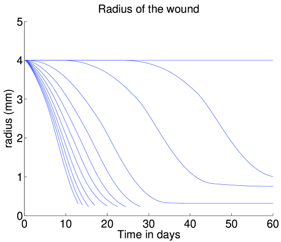
Fig. 1: The radius of the wound as a function of time for different values of $\gamma$. From left to right: $\gamma=0,0.1,0.2,\ldots,0.8,0.9,0.92,0.95,1$. Other parameters used are the same as in [28]; the nondimensionalized values are: $L=5$, $R_{0}=8/3$, $\rho_{m}=2$, $K_{w\rho}=K_{wf}0.25$, $k_{\rho}=5/16$, $\lambda_{\rho}=0.1$, $\beta=10$, $D_{w}=0.5$, $D_{p}=D_{e}=1$, $D_{m}=D_{f}=5\times 10^{-2}$, $D_{n}=10^{-3}$, $D_{b}=7\times 10^{-4}$, $\chi_{m}=\chi_{f}=0.1$, $\chi_{n}=1$, $m_{m}=f_{m}=n_{m}=10$, $A=0.1$, $w_{b}=2$, $k_{w}=4.39$, $\lambda_{wf}=0.227$, $\lambda_{wm}=4.16$, $\lambda_{d}=2$, $k_{f}=5.78\times 10^{-3}$, $\lambda_{f}=5.2\times 10^{-3}$, $k_{nb}=k_{n}=k_{b}/10=2.16\times 10^{-2}$, $\lambda_{nn}=100\lambda_{nb}=2.25$, $k_{sg}=6.25\times 10^{-2}$.

We conjecture that if the parameters of the system (2.2) – (2.28) are chosen on the basis of experimental results, as in [28], then there exists a parameter value $\gamma_{\ast}$ such that (8.1) holds if $\gamma_{\ast}<\gamma\leq 1$ and

$$\lim_{t\to\infty}R_{\gamma}(t)=0\quad\text{if}\;\;\gamma<\gamma_{\ast}.$$

If this conjecture is true then, in particular,

$$\lim_{t\to\infty}R_{\gamma}(t)=0\quad\text{if}\;\;\gamma=0.$$

But even this assertion is still an open question. We can only prove, for the system $($2.2$)$ – $($2.28$)$, with general parameters, the following result.

Theorem 9.1.

If $\gamma=0$, then

$$\rho(L,t)>1,\hskip 20.00003pt0<t<\infty,$$ (9.1)

$$\dot{R}(t)<0,\hskip 20.00003pt0<t<\infty,$$ (9.2)

$$Q(t)>0,\hskip 20.00003pt0<t<\infty.$$ (9.3)

Proof. Using the boundary conditions $w(L,t)=1,\;f(L,t)=1$, $v(L,t)=0$ and $($2.26$)$, we obtain from $($2.2$)$ at $r=L$ the relation

$$\dfrac{\partial\rho(L,t)}{\partial t}+\rho(L,t)\dfrac{\partial v}{\partial r}(L,t) = \frac{k_{\rho}}{1+K_{w\rho}}\left(1-\frac{\rho}{\rho_{m}}\right)-\frac{k_{\rho}}{1+K_{w\rho}}\left(1-\frac{1}{\rho_{m}}\right)\rho$$

$$= -\frac{k_{\rho}}{1+K_{w\rho}}(\rho-1),$$

and from $($3.8$)$,

$$\dfrac{\partial v}{\partial r}(L,t)=P(L,t)-\frac{2}{L^{2}+R^{2}(t)}Q(t).$$

Hence,

$$\frac{\partial\rho(L,t)}{\partial t}=-c_{0}\Big{(}\rho(L,t)-1\Big{)}-\beta\rho(L,t)\Big{(}\rho(L,t)-1\Big{)}_{+}+\frac{2\rho(L,t)}{L^{2}+R(t)^{2}}Q(t).$$ (9.4)

where $c_{0}$ is a positive constant.

Using the initial conditions

$$\rho(r,0)\equiv 1,\hskip 10.00002ptw(r,0)\equiv 1,\hskip 10.00002ptf(r,0)\equiv 1,\hskip 10.00002ptm(r,0)\equiv 0,\hskip 10.00002ptv(r,0)\equiv 0\hskip 10.00002pt\text{for }R_{0}<r<L,$$

$$b(r,0)\equiv 1,\hskip 10.00002ptp(r,0)\equiv 0\hskip 10.00002pt\text{for }R_{0}+\varepsilon_{0}\leqslant r<L,$$

in $($2.2$)$ and $($2.4$)$ and recalling the relations (2.26) and (2.27), we find that

$$\frac{\partial\rho(r,0)}{\partial t}\equiv 0,\hskip 20.00003ptR_{0}<r<L,$$ (9.5)

$$\frac{\partial w(r,0)}{\partial t}\equiv 0,\hskip 20.00003ptR_{0}+\varepsilon_{0}\leqslant r<L.$$ (9.6)

Using $($2.25$)$ we also obtain (upon recalling $($2.28$)$) that

$$\frac{\partial f(r,0)}{\partial t}=\frac{\chi_{f}}{r}H(1-\frac{1}{f_{m}})p_{0}^{\prime}(r)\Big{/}\sqrt{1+k_{sg}\Big{(}\frac{k_{pb}}{D_{p}}\Big{)}^{2}}>0,\hskip 20.00003ptR_{0}<r<R_{0}+\varepsilon_{0}.$$ (9.7)

Differentiating Equation (2.2) in $t$ and using (9.5) – (9.7) and the $C_{r,t}^{2+\alpha,1+\alpha/2}$ regularity of $w$, we deduce that

$$\frac{\partial^{2}\rho(r_{0},0)}{\partial t^{2}}>0\quad\mbox{for}\;\;0<R_{0}+\varepsilon_{0}-r_{0}\ll 1$$

This implies that , for $0<R_{0}+\varepsilon_{0}-r_{0}\ll 1$ and $0<t\ll 1$,

$$\rho(r_{0},t)>1,$$

and hence

$$Q(t)>0\hskip 10.00002pt\text{for }0<t\ll 1.$$ (9.8)

Since $\rho(0,L)=1$, from $($9.4$)$ and $($9.5$)$ it follows that

$$\rho(0,t)>1$$ (9.9)

for all $0<t<\infty$. This in turn implies that $Q(t)>1$ for all $0<t<\infty$, hence $\dot{R}(t)<0$ and (by (9.4)) $\rho(L,t)>1$ for all $0<t<\infty$.       

10 Conclusion

In this paper we established existence and uniqueness of a solution to a free boundary problem which models ischemic wound healing. The ischemic condition is described in terms of a parameter $\gamma$ ($0\leq\gamma\leq 1$) which appears as a coefficient in a Robin boundary condition for the various cells and chemical densities. We also proved that under extreme ischemic conditions ($\gamma$ near 1) the open wound stops decreasing in finite time. When the parameters of the system are taken on the basis of biological experiments, simulations show that there is a parameter $\gamma_{\ast}$ such that the wound heals if $0\leq\gamma<\gamma_{\ast}$ and does not heal if $\gamma_{\ast}<\gamma\leq 1$. This assertion remains a challenging mathematical open problem. Future work should include the introduction of pressure and diabetic conditions in ischemic wounds, as well as inflammatory conditions.

Acknowledgment. This work was partially supported by National Science Foundation upon agreement No. 0635561 and the National Institute of Health (OD) Award UL1RR025755.

References

[1]D. B. Allen, J. J. Maguire, M. Mahdavian, C. Wicke, L. Marcocci,
H. Scheuenstuhl, M. Chang, A. X. Le, H. W. Hopf, and T. K. Hunt, Wound
hypoxia and acidosis limit neutrophil bacterial killing mechanisms, Arch
Surg, 132 (1997), pp. 991–996.
[2]A. R. A. Anderson and M. A. J. Chaplain, Continuous and discrete
mathematical models of tumor-induced angiogenesis, Bull Math Biol, 60
(1998), pp. 857–899.
[3]H. M. Byrne, M. A. J. Chaplain, D. L. Evans, and I. Hopkinson, Mathematical modelling of angiogenesis in wound healing: Comparison of theory
and experiment., J. Theor. Med., 2 (2000), pp. 175–197.
[4]S. Colgan, S. Mukherjee, and P. Major, Hypoxia-induced lactate
dehydrogenase expression and tumor angiogenesis, Clinical Colorectal Cancer,
6 (2007), pp. 442–446.
[5]Y. Dor, V. Djonov, and E. Keshet, Induction of vascular networks in
adult organs: Implications to proangiogenic therapy, Annals of the New York
Academy of Sciences, 995 (2003), pp. 208–216.
[6], Making vascular
networks in the adult: branching morphogenesis without a roadmap, Trends in
Cell Biology, 13 (2003), pp. 131 – 136.
[7]Avner Friedman, Partial Differential Equations of Parabolic Type,
Dover Publications, Mineola , New York, Apr 2008.
[8]A. Friedman, C. Huang, and J. Yong, Effective permeability of the
boundary of a domain, Communications in Partial Differential Equations, 20
(1995), pp. 59–102.
[9]Avner Friedman and Georgios Lolas, Analysis of a mathematical model
of tumor lymphangiogenesis, M3AS, 15 (2005), pp. 95–107.
[10]J. J. Gibson, A. Angeles, and T. Hunt, Increased oxygen tension
potentiates angiogenesis, Surg Forum, 87 (1997), pp. 696–699.
[11]G. M. Gordillo and C. K. Sen, Revisiting the essential role of
oxygen in wound healing, Am. J. Surg., 186 (2003), pp. 259–263.
[12]H. W. Hopf, J. J. Gibson, A. P. Angeles, J. S. Constant, J. J. Feng, M. D.
Rollins, H. M. Zamirul, and T. K. Hunt, Hyperoxia and angiogenesis,
Wound Repair and Regeneration, 13 (2005), pp. 558–564.
[13]J. J. Hutton, A. L. Tappel, and S. Udenfriend, Cofactor and
substrate requirements of collagen proline hydroxylase, Arch Biochem
Biophys, 118 (1967), pp. 231–40.
[14]D. Liao and R. S. Johnson, Hypoxia: A key regulator of angiogenesis
in cancer, Cancer and Metastasis Reviews, 26 (2007), pp. 281–290.
[15]Gary M. Lieberman, Second Order Parabolic Differential Equations,
World Scientific Publishing Company, 1996.
[16]S. R. McDougall, A. R. A. Anderson, M. A. J. Chaplain, and J. A.
Sherratt, Mathematical modelling of flow through vascular networks:
Implications for tumour-induced angiogenesis and chemotherapy strategies,
Bull. Math. Biol., 64 (2002), pp. 673–702.
[17]R. Myllyla, L. Tuderman, and K. I. Kivirikko, Mechanism of the
prolyl hydroxylase reaction, European Journal of Biochemistry, 80 (1977),
pp. 349–357.
[18]M. Oberringer, M. Jennevein, S. E. Matsch, T. Pohlemann, and A. Seekamp,
Different cell cycle responses of wound healing protagonists to
transient in vitro hypoxia, Histochemistry and Cell Biology, 123 (2005),
pp. 595–603.
[19]G. Pettet, M. A. J. Chaplain, D. L. S. Mcelwain, and H. M. Byrne, On
the role of angiogenesis in wound healing, Proc. R. Soc. Lond. B, 263
(1996), pp. 1487–1493.
[20]G. J. Pettet, H. M. Byrne, D. L. S. Mcelwain, and J. Norbury, A
model of wound-healing angiogenesis in soft tissue, Mathematical
Biosciences, 136 (1996), pp. 35 – 63.
[21]C. W. Pugh and P. J. Ratcliffe, Regulation of angiogenesis by
hypoxia: role of the HIF system, Nat Med, 9 (2003), pp. 677–684.
[22]S. Roy, S. B., S. K., G. Gordillo, V. Bergdall, J. Green, C. B. Marsh,
L. J. Gould, and C. K. Sen, Characterization of a pre-clinical model of
chronic ischemic wound, Physiol Genomics, (2009).
[23]M. Safran and W. G. J. Kaelin, HIF hydroxylation and the mammalian
oxygen-sensing pathway, J. Clin. Invest., 111 (2003), pp. 779–783.
[24]R. C. Schugart, A. Friedman, R. Zhao, and C. K. Sen, Wound
angiogenesis as a function of tissue oxygen tension: A mathematical model,
PNAS, 105 (2008), pp. 2628–2633.
[25]G. L. Semenza, HIF-1: Using two hands to flip the angiogenic
switch, Cancer and Metastasis Reviews, 19 (2000), pp. 59–65.
Review.
[26]C. K. Sen, Wound healing essentials: Let there be oxygen, Wound
Repair and Regeneration, 17 (2009), pp. 1–18.
[27]A. Stephanou, S.R. McDougall, A.R.A. Anderson, and M.A.J. Chaplain, Mathematical modelling of flow in 2d and 3d vascular networks: Applications
to anti-angiogenic and chemotherapeutic drug strategies, Mathematical and
Computer Modelling, 41 (2005), pp. 1137 – 1156.
[28]C. Xue, A. Friedman, and C. K. Sen, A mathematical model of ischemic
cutaneous wounds, PNAS, in press, (2009).