On linear degeneracy of integrable quasilinear systems in higher dimensions

E.V. Ferapontov, K.R. Khusnutdinova and C. Kleinโˆ—
Abstract

We investigate (d+1)๐‘‘1(d+1)-dimensional quasilinear systems which are integrable by the method of hydrodynamic reductions. In the case dโ‰ฅ3๐‘‘3d\geq 3 we formulate a conjecture that any such system with an irreducible dispersion relation must be linearly degenerate. We prove this conjecture in the 222-component case, providing a complete classification of multi-dimensional integrable systems in question. In particular, our results imply the non-existence of 222-component integrable systems of hydrodynamic type for dโ‰ฅ6๐‘‘6d\geq 6.

In the second half of the paper we discuss a numerical and analytical evidence for the impossibility of the breakdown of smooth initial data for linearly degenerate systems in 2+1212+1 dimensions.


MSC: 35L40, 35L65, 37K10.


Keywords: Multi-dimensional Quasilinear Systems, Hydrodynamic Reductions, Integrability, Linear Degeneracy, Cauchy Problem, Classical Solutions.

Department of Mathematical Sciences

Loughborough University

Loughborough, Leicestershire LE11 3TU

United Kingdom

โˆ— Institut de Mathรฉmatiques de Bourgogne

9 avenue Alain Savary, BP 47870

21078 Dijon Cedex, France

e-mails:

E.V.Ferapontov@lboro.ac.uk
K.Khusnutdinova@lboro.ac.uk
Christian.Klein@u-bourgogne.fr


1 Introduction

In this paper we discuss (d+1)๐‘‘1(d+1)-dimensional quasilinear systems of the form

๐ฎt+โˆ‘i=1dAiโ€‹(๐ฎ)โ€‹๐ฎxi=0,subscript๐ฎ๐‘กsuperscriptsubscript๐‘–1๐‘‘subscript๐ด๐‘–๐ฎsubscript๐ฎsuperscript๐‘ฅ๐‘–0{\bf u}_{t}+\sum_{i=1}^{d}A_{i}({\bf u}){\bf u}_{x^{i}}=0, (1)

where t,xi๐‘กsuperscript๐‘ฅ๐‘–t,x^{i} are independent variables, ๐ฎ๐ฎ{\bf u} is an n๐‘›n-component column vector and Aiโ€‹(๐ฎ)subscript๐ด๐‘–๐ฎA_{i}({\bf u}) are nร—n๐‘›๐‘›n\times n matrices. Systems of this type play an important role in continuum mechanics and physics, and there is a vast literature covering their analytical, geometric and applied aspects, see e.g. [7, 24, 36, 37, 19, 8, 42]. In this paper we assume that the dispersion relation det(ฮผโ€‹I+ฮฑiโ€‹Ai)=0๐œ‡๐ผsuperscript๐›ผ๐‘–subscript๐ด๐‘–0\det(\mu I+\alpha^{i}A_{i})=0 defines an irreducible algebraic variety (for n=2๐‘›2n=2, an irreducible quadric) in the variables ฮผ,ฮฑi๐œ‡superscript๐›ผ๐‘–\mu,\ \alpha^{i}. Our prime goal is the classification of integrable systems of the form (1) in any dimension.

For d=1๐‘‘1d=1, any two-component system of the form

๐ฎt+Aโ€‹(๐ฎ)โ€‹๐ฎx=0subscript๐ฎ๐‘ก๐ด๐ฎsubscript๐ฎ๐‘ฅ0{\bf u}_{t}+A({\bf u}){\bf u}_{x}=0

is linearizable by a hodograph transformation which interchanges the dependent and independent variables and, therefore, is automatically integrable. In particular, any such system possesses an infinity of conservation laws and commuting flows.

For d=2๐‘‘2d=2,

๐ฎt+Aโ€‹(๐ฎ)โ€‹๐ฎx+Bโ€‹(๐ฎ)โ€‹๐ฎy=0,subscript๐ฎ๐‘ก๐ด๐ฎsubscript๐ฎ๐‘ฅ๐ต๐ฎsubscript๐ฎ๐‘ฆ0{\bf u}_{t}+A({\bf u}){\bf u}_{x}+B({\bf u}){\bf u}_{y}=0, (2)

the situation is more subtle. Even the very concept of integrability for multi-dimensional systems of the form (1) requires an alternative approach. Such approach, based on the method of hydrodynamic reductions, was outlined in [13]. It was proposed to call a (2+1)21(2+1)-dimensional system integrable if it possesses infinitely many multi-phase solutions of the form ๐ฎ=๐ฎโ€‹(R1,โ€ฆ,RN)๐ฎ๐ฎsuperscript๐‘…1โ€ฆsuperscript๐‘…๐‘{\bf u}={\bf u}(R^{1},...,R^{N}) where the phases Riโ€‹(x,y,t)superscript๐‘…๐‘–๐‘ฅ๐‘ฆ๐‘กR^{i}(x,y,t) satisfy a pair of commuting hydrodynamic type systems

Rti=ฮปiโ€‹(R)โ€‹Rxi,Ryi=ฮผiโ€‹(R)โ€‹Rxi;formulae-sequencesubscriptsuperscript๐‘…๐‘–๐‘กsuperscript๐œ†๐‘–๐‘…subscriptsuperscript๐‘…๐‘–๐‘ฅsubscriptsuperscript๐‘…๐‘–๐‘ฆsuperscript๐œ‡๐‘–๐‘…subscriptsuperscript๐‘…๐‘–๐‘ฅR^{i}_{t}=\lambda^{i}(R)\ R^{i}_{x},~{}~{}~{}~{}R^{i}_{y}=\mu^{i}(R)\ R^{i}_{x}; (3)

we emphasize that the number of phases N๐‘N is allowed to be arbitrary. In what follows, we will refer to the equations (3) as N๐‘N-component hydrodynamic reductions. Multi-phase solutions of this type, known in gas dynamics as nonlinear interactions of planar simple waves, date back to [41, 6, 34, 20]. Their first appearance in the context of integrable systems and, in particular, the dispersionless Kadomtsev-Petviashvili hierarchy, is due to [17, 18]. The requirement of the existence of multi-phase solutions imposes strong constraints on the matrices Aโ€‹(๐ฎ)๐ด๐ฎA({\bf u}) and Bโ€‹(๐ฎ)๐ต๐ฎB({\bf u}). In the two-component case these integrability conditions were derived in [14], and are included in Sect. 4.1 of this paper. In particular, they imply that any integrable system of this kind is necessarily conservative, and possesses a dispersionless Lax pair. It was demonstrated in [30, 31] that the integrability conditions can be resolved in generalized hypergeometric functions.

Remarkably, for dโ‰ฅ3๐‘‘3d\geq 3 the situation simplifies dramatically: the requirement of the integrability proves to be too strong, so that very few examples survive in many dimensions. According to the definition proposed in [15], a (d+1)๐‘‘1(d+1)-dimensional system of the form (1) is said to be integrable if it possesses infinitely many N๐‘N-component hydrodynamic reductions parametrized by (dโˆ’1)โ€‹N๐‘‘1๐‘(d-1)N arbitrary functions of one variable. Here by a hydrodynamic reduction we mean a decomposition of a (d+1)๐‘‘1(d+1)-dimensional system into d๐‘‘d commuting systems of the form (3). Although the derivation of the integrability conditions based on the method of hydrodynamic reductions leads to a quite complicated analysis, there exists a simple way to bypass lengthy calculations. It is based on the requirement that all traveling wave reductions of a (d+1)๐‘‘1(d+1)-dimensional integrable system to (2+1)21(2+1)-dimensional systems should be themselves integrable. Since the integrability conditions in 2+1212+1 dimensions are explicitly known, this provides a set of strong constraints which are therefore necessary for the integrability. In fact, in our case they turn out to be sufficient. Our main result is the following

Theorem 1

There exist no two-component integrable systems of the form (1) in dimensions 6+1616+1 and higher. In 5+1515+1 dimensions, there exists a unique integrable system. Up to linear transformations of the independent variables, it can be brought to the form

vt=wx+wโ€‹vrโˆ’vโ€‹wr,wz=vy+vโ€‹wsโˆ’wโ€‹vs.formulae-sequencesubscript๐‘ฃ๐‘กsubscript๐‘ค๐‘ฅ๐‘คsubscript๐‘ฃ๐‘Ÿ๐‘ฃsubscript๐‘ค๐‘Ÿsubscript๐‘ค๐‘งsubscript๐‘ฃ๐‘ฆ๐‘ฃsubscript๐‘ค๐‘ ๐‘คsubscript๐‘ฃ๐‘ v_{t}=w_{x}+wv_{r}-vw_{r},~{}~{}~{}~{}w_{z}=v_{y}+vw_{s}-wv_{s}. (4)

In 4+1414+1 and 3+1313+1 dimensions, any two-component integrable system can be obtained as a traveling wave reduction of the system (4).

The proof of this result is given in Sect. 4.2. The system (4) first appeared in [15], see Sect. 2 for more details. An important property of this example is its linear degeneracy. Recall that a matrix Aโ€‹(๐ฎ)๐ด๐ฎA({\bf u}) is said to be linearly degenerate if its eigenvalues (assumed real and distinct) are constant in the direction of the corresponding eigenvectors. Explicitly, Lriโ€‹ฮปi=0subscript๐ฟsuperscript๐‘Ÿ๐‘–superscript๐œ†๐‘–0L_{r^{i}}\lambda^{i}=0, no summation, where Lrisubscript๐ฟsuperscript๐‘Ÿ๐‘–L_{r^{i}} is the Lie derivative in the direction of the eigenvector risuperscript๐‘Ÿ๐‘–r^{i}, and Aโ€‹ri=ฮปiโ€‹ri๐ดsuperscript๐‘Ÿ๐‘–superscript๐œ†๐‘–superscript๐‘Ÿ๐‘–Ar^{i}=\lambda^{i}r^{i}. A system of the form (1) is said to be linearly degenerate (totally linearly degenerate in the terminology of [24]), if any matrix Aโ€‹(๐ฎ)=ฮฑiโ€‹Aiโ€‹(๐ฎ)๐ด๐ฎsuperscript๐›ผ๐‘–subscript๐ด๐‘–๐ฎA({\bf u})=\alpha^{i}A_{i}({\bf u}) is linearly degenerate for any values of the constants ฮฑisuperscript๐›ผ๐‘–\alpha^{i}. Theorem 1 and other existing examples support the following conjecture.

Conjecture. For dโ‰ฅ3๐‘‘3d\geq 3, any n๐‘›n-component (d+1)๐‘‘1(d+1)-dimensional integrable system of the form (1) with an irreducible dispersion relation must be linearly degenerate.

According to the conjecture of Majda [24], p. 89, linearly degenerate systems are quite exceptional from the point of view of the global solvability of the Cauchy problem: the shock wave formation, which is a standard scenario for genuinely nonlinear systems, never happens for smooth initial data. Although this fact is well-established in 1+1111+1 dimensions [35, 36, 23, 37], the multi-dimensional situation is still out of reach. We refer to the recent work [25, 26, 27] which utilizes a novel version of the inverse scattering transform to investigate the breakdown phenomena for some (2+1)21(2+1)-dimensional dispersionless integrable models. In Sect. 3 we provide some further analytical and numerical evidence in support of Majdaโ€™s conjecture. As an example, we choose a particular (2+1)21(2+1)-dimensional traveling wave reduction of the system (4), namely,

vt+wx=0,wt+wy+vโ€‹wxโˆ’wโ€‹vx=0,formulae-sequencesubscript๐‘ฃ๐‘กsubscript๐‘ค๐‘ฅ0subscript๐‘ค๐‘กsubscript๐‘ค๐‘ฆ๐‘ฃsubscript๐‘ค๐‘ฅ๐‘คsubscript๐‘ฃ๐‘ฅ0v_{t}+w_{x}=0,~{}~{}~{}~{}w_{t}+w_{y}+vw_{x}-wv_{x}=0, (5)

see Sect. 3.1 for the discussion of this example. In a somewhat different form, it appeared in [39]. In Sections 3.2โ€“3.3, applying the method of hydrodynamic reductions and other simple techniques, we construct some global exact solutions of the system (5). In Sect. 3.4 we summarize the results of numerical simulations based on the Friedrichs-symmetrized representation of the system (5). These results clearly indicate that hump-like initial data tend to spread out, and do not break down in finite time.

2 Examples of multi-dimensional integrable systems

In this section we list some examples of integrable (d+1)๐‘‘1(d+1)-dimensional quasilinear systems of the form (1) for dโ‰ฅ3๐‘‘3d\geq 3. All such systems turn out to be linearly degenerate, namely, an arbitrary matrix of the linear pencil Aโ€‹(๐ฎ)=ฮฑiโ€‹Aiโ€‹(๐ฎ)๐ด๐ฎsuperscript๐›ผ๐‘–subscript๐ด๐‘–๐ฎA({\bf u})=\alpha^{i}A_{i}({\bf u}), where ฮฑisuperscript๐›ผ๐‘–\alpha^{i} are arbitrary constants, must be linearly degenerate (totally linearly degenerate systems in the terminology of [24]). We recall that there exists a useful criterion of linear degeneracy which can be summarized as follows. Given a matrix Aโ€‹(๐ฎ)๐ด๐ฎA({\bf u}), let us introduce its characteristic polynomial,

dโ€‹eโ€‹tโ€‹(ฮปโ€‹Eโˆ’Aโ€‹(๐ฎ))=ฮปn+f1โ€‹(๐ฎ)โ€‹ฮปnโˆ’1+f2โ€‹(๐ฎ)โ€‹ฮปnโˆ’2+โ€ฆ+fnโ€‹(๐ฎ).๐‘‘๐‘’๐‘ก๐œ†๐ธ๐ด๐ฎsuperscript๐œ†๐‘›subscript๐‘“1๐ฎsuperscript๐œ†๐‘›1subscript๐‘“2๐ฎsuperscript๐œ†๐‘›2โ€ฆsubscript๐‘“๐‘›๐ฎdet(\lambda E-A({\bf u}))={\lambda}^{n}+f_{1}({\bf u}){\lambda}^{n-1}+f_{2}({\bf u}){\lambda}^{n-2}+\ldots+f_{n}({\bf u}).

The condition of linear degeneracy is given by [12],

โˆ‡f1โ€‹Anโˆ’1+โˆ‡f2โ€‹Anโˆ’2+โ€ฆ+โˆ‡fn=0,โˆ‡subscript๐‘“1superscript๐ด๐‘›1โˆ‡subscript๐‘“2superscript๐ด๐‘›2โ€ฆโˆ‡subscript๐‘“๐‘›0\nabla f_{1}~{}A^{n-1}+\nabla f_{2}~{}A^{n-2}+\ldots+\nabla f_{n}=0, (6)

where โˆ‡โˆ‡\nabla is the operator of the gradient, โˆ‡f=(โˆ‚fโˆ‚u1,โ€ฆ,โˆ‚fโˆ‚un)โˆ‡๐‘“๐‘“superscript๐‘ข1โ€ฆ๐‘“superscript๐‘ข๐‘›\nabla f=({{\partial f}\over{\partial u^{1}}},\ldots,{{\partial f}\over{\partial u^{n}}}), and Aksuperscript๐ด๐‘˜A^{k} denotes k๐‘˜k-th power of the matrix A๐ดA. Our first example plays a key role in the classification of two-component multi-dimensional quasilinear systems.

Example 1. The six-dimensional two-component integrable system (4),

vt=wx+wโ€‹vrโˆ’vโ€‹wr,wz=vy+vโ€‹wsโˆ’wโ€‹vs,formulae-sequencesubscript๐‘ฃ๐‘กsubscript๐‘ค๐‘ฅ๐‘คsubscript๐‘ฃ๐‘Ÿ๐‘ฃsubscript๐‘ค๐‘Ÿsubscript๐‘ค๐‘งsubscript๐‘ฃ๐‘ฆ๐‘ฃsubscript๐‘ค๐‘ ๐‘คsubscript๐‘ฃ๐‘ v_{t}=w_{x}+wv_{r}-vw_{r},~{}~{}~{}~{}w_{z}=v_{y}+vw_{s}-wv_{s},

first appeared in [15]. It can also be obtained as the condition of commutativity of two parameter-dependent vector fields,

[โˆ‚zโˆ’vโ€‹โˆ‚sโˆ’ฮปโ€‹โˆ‚x+ฮปโ€‹vโ€‹โˆ‚r,โˆ‚yโˆ’wโ€‹โˆ‚sโˆ’ฮปโ€‹โˆ‚t+ฮปโ€‹wโ€‹โˆ‚r]=0.subscript๐‘ง๐‘ฃsubscript๐‘ ๐œ†subscript๐‘ฅ๐œ†๐‘ฃsubscript๐‘Ÿsubscript๐‘ฆ๐‘คsubscript๐‘ ๐œ†subscript๐‘ก๐œ†๐‘คsubscript๐‘Ÿ0[\partial_{z}-v\partial_{s}-\lambda\partial_{x}+\lambda v\partial_{r},~{}~{}\partial_{y}-w\partial_{s}-\lambda\partial_{t}+\lambda w\partial_{r}]=0.

It was demonstrated in [15] that system (4) possesses infinitely many n๐‘›n-component hydrodynamic reductions parametrized by 4โ€‹n4๐‘›4n arbitrary functions of one variable. This example is a result of the following construction. In [14], we proposed a characterization of two-component (2+1)21(2+1)-dimensional integrable systems of the form

(vw)t+Aโ€‹(v,w)โ€‹(vw)x+Bโ€‹(v,w)โ€‹(vw)y=0.subscript๐‘ฃ๐‘ค๐‘ก๐ด๐‘ฃ๐‘คsubscript๐‘ฃ๐‘ค๐‘ฅ๐ต๐‘ฃ๐‘คsubscript๐‘ฃ๐‘ค๐‘ฆ0\left(\begin{array}[]{c}v\\ w\end{array}\right)_{t}+A(v,w)\left(\begin{array}[]{c}v\\ w\end{array}\right)_{x}+B(v,w)\left(\begin{array}[]{c}v\\ w\end{array}\right)_{y}=0.

The integrability conditions constitute a complicated overdetermined system of second order PDEs for the 2ร—2222\times 2 matrices A๐ดA and B๐ตB which are presented in Sect. 4.1. In the particular case when A๐ดA is taken to be linearly degenerate,

A=(w00v),๐ด๐‘ค0missing-subexpressionmissing-subexpression0๐‘ฃA=\left(\begin{array}[]{cc}w&0\\ \\ 0&v\end{array}\right), (7)

the integrability conditions imply the following generic expression for B๐ตB,

B=(fโ€‹(w)wโˆ’vโˆ’ฮฑโ€‹w2fโ€‹(v)wโˆ’vfโ€‹(w)vโˆ’wfโ€‹(v)vโˆ’wโˆ’ฮฑโ€‹v2),๐ต๐‘“๐‘ค๐‘ค๐‘ฃ๐›ผsuperscript๐‘ค2๐‘“๐‘ฃ๐‘ค๐‘ฃmissing-subexpressionmissing-subexpression๐‘“๐‘ค๐‘ฃ๐‘ค๐‘“๐‘ฃ๐‘ฃ๐‘ค๐›ผsuperscript๐‘ฃ2B=\left(\begin{array}[]{cc}\frac{f(w)}{w-v}-\alpha w^{2}&\frac{f(v)}{w-v}\\ \\ \frac{f(w)}{v-w}&\frac{f(v)}{v-w}-\alpha v^{2}\end{array}\right), (8)

where f๐‘“f is a cubic polynomial, fโ€‹(v)=ฮฑโ€‹v3+ฮฒโ€‹v2+ฮณโ€‹v+ฮด๐‘“๐‘ฃ๐›ผsuperscript๐‘ฃ3๐›ฝsuperscript๐‘ฃ2๐›พ๐‘ฃ๐›ฟf(v)=\alpha v^{3}+\beta v^{2}+\gamma v+\delta, and ฮฑ,ฮฒ,ฮณ,ฮด๐›ผ๐›ฝ๐›พ๐›ฟ\alpha,\beta,\gamma,\delta are arbitrary constants. A remarkable property of this example is that any matrix in the linear pencil B+ฮผโ€‹A๐ต๐œ‡๐ดB+\mu A is also linearly degenerate. Explicitly, one has

B=ฮดโ€‹B1+ฮณโ€‹B2+ฮฒโ€‹B3+ฮฑโ€‹B4=ฮดโ€‹(1wโˆ’v1wโˆ’v1vโˆ’w1vโˆ’w)+ฮณโ€‹(wwโˆ’vvwโˆ’vwvโˆ’wvvโˆ’w)+ฮฒโ€‹(w2wโˆ’vv2wโˆ’vw2vโˆ’wv2vโˆ’w)+ฮฑโ€‹(vโ€‹w2wโˆ’vv3wโˆ’vw3vโˆ’wwโ€‹v2vโˆ’w).๐ต๐›ฟsubscript๐ต1๐›พsubscript๐ต2๐›ฝsubscript๐ต3๐›ผsubscript๐ต4absentmissing-subexpression๐›ฟ1๐‘ค๐‘ฃ1๐‘ค๐‘ฃ1๐‘ฃ๐‘ค1๐‘ฃ๐‘ค๐›พ๐‘ค๐‘ค๐‘ฃ๐‘ฃ๐‘ค๐‘ฃ๐‘ค๐‘ฃ๐‘ค๐‘ฃ๐‘ฃ๐‘ค๐›ฝsuperscript๐‘ค2๐‘ค๐‘ฃsuperscript๐‘ฃ2๐‘ค๐‘ฃsuperscript๐‘ค2๐‘ฃ๐‘คsuperscript๐‘ฃ2๐‘ฃ๐‘ค๐›ผ๐‘ฃsuperscript๐‘ค2๐‘ค๐‘ฃsuperscript๐‘ฃ3๐‘ค๐‘ฃsuperscript๐‘ค3๐‘ฃ๐‘ค๐‘คsuperscript๐‘ฃ2๐‘ฃ๐‘ค\begin{array}[]{c}B=\delta B_{1}+\gamma B_{2}+\beta B_{3}+\alpha B_{4}=\\ \\ \delta\left(\begin{array}[]{cc}\frac{1}{w-v}&\frac{1}{w-v}\\ \frac{1}{v-w}&\frac{1}{v-w}\end{array}\right)+\gamma\left(\begin{array}[]{cc}\frac{w}{w-v}&\frac{v}{w-v}\\ \frac{w}{v-w}&\frac{v}{v-w}\end{array}\right)+\beta\left(\begin{array}[]{cc}\frac{w^{2}}{w-v}&\frac{v^{2}}{w-v}\\ \frac{w^{2}}{v-w}&\frac{v^{2}}{v-w}\end{array}\right)+\alpha\left(\begin{array}[]{cc}\frac{vw^{2}}{w-v}&\frac{v^{3}}{w-v}\\ \frac{w^{3}}{v-w}&\frac{wv^{2}}{v-w}\end{array}\right).\end{array}

Let us introduce the (5+1)51(5+1)-dimensional system

(vw)t+Aโ€‹(vw)x+B1โ€‹(vw)y+B2โ€‹(vw)z+B3โ€‹(vw)s+B4โ€‹(vw)r=0.subscript๐‘ฃ๐‘ค๐‘ก๐ดsubscript๐‘ฃ๐‘ค๐‘ฅsubscript๐ต1subscript๐‘ฃ๐‘ค๐‘ฆsubscript๐ต2subscript๐‘ฃ๐‘ค๐‘งsubscript๐ต3subscript๐‘ฃ๐‘ค๐‘ subscript๐ต4subscript๐‘ฃ๐‘ค๐‘Ÿ0\left(\begin{array}[]{c}v\\ w\end{array}\right)_{t}+A\left(\begin{array}[]{c}v\\ w\end{array}\right)_{x}+\\ \ \\ B_{1}\left(\begin{array}[]{c}v\\ w\end{array}\right)_{y}+B_{2}\left(\begin{array}[]{c}v\\ w\end{array}\right)_{z}+B_{3}\left(\begin{array}[]{c}v\\ w\end{array}\right)_{s}+B_{4}\left(\begin{array}[]{c}v\\ w\end{array}\right)_{r}=0.

Notice that an arbitrary linear combination of matrices A๐ดA and B1,B2,B3,B4subscript๐ต1subscript๐ต2subscript๐ต3subscript๐ต4B_{1},B_{2},B_{3},B_{4} is automatically linearly degenerate. This can be verified directly using the criterion (6). In the new variables V=v+w,W=vโ€‹wformulae-sequence๐‘‰๐‘ฃ๐‘ค๐‘Š๐‘ฃ๐‘คV=v+w,\ W=vw, our system reduces to

Vt+Wx+Wโ€‹Vrโˆ’Vโ€‹Wr=0,Wt+Vโ€‹Wxโˆ’Wโ€‹Vx+Vy+Wz+Vโ€‹Wsโˆ’Wโ€‹Vs=0,formulae-sequencesubscript๐‘‰๐‘กsubscript๐‘Š๐‘ฅ๐‘Šsubscript๐‘‰๐‘Ÿ๐‘‰subscript๐‘Š๐‘Ÿ0subscript๐‘Š๐‘ก๐‘‰subscript๐‘Š๐‘ฅ๐‘Šsubscript๐‘‰๐‘ฅsubscript๐‘‰๐‘ฆsubscript๐‘Š๐‘ง๐‘‰subscript๐‘Š๐‘ ๐‘Šsubscript๐‘‰๐‘ 0V_{t}+W_{x}+WV_{r}-VW_{r}=0,~{}~{}~{}W_{t}+VW_{x}-WV_{x}+V_{y}+W_{z}+VW_{s}-WV_{s}=0,

taking a fully symmetric form (4) after an obvious linear transformation of the independent variables. We would like to emphasize that there was no a priori reason for the (5+1)51(5+1)-dimensional system obtained in this way to be integrable: this is a miracle which is due to the linear degeneracy. Notice that a particular dimensional reduction of the system (4),

mt=nx,nt=my+mโ€‹nxโˆ’nโ€‹mx,formulae-sequencesubscript๐‘š๐‘กsubscript๐‘›๐‘ฅsubscript๐‘›๐‘กsubscript๐‘š๐‘ฆ๐‘šsubscript๐‘›๐‘ฅ๐‘›subscript๐‘š๐‘ฅm_{t}=n_{x},~{}~{}~{}~{}n_{t}=m_{y}+mn_{x}-nm_{x}, (9)

known as the Pavlov equation, has been extensively discussed in the context of hydrodynamic chains and the โ€˜universal hierarchyโ€™ [33, 39, 40, 27].

Example 2. The following four-dimensional three-component integrable system appeared in [11] in the context of hyper-Hermitian conformal structures,

Aโ€‹๐x+B1โ€‹๐y1+B2โ€‹๐y2+B3โ€‹๐y3=0,๐ดsubscript๐๐‘ฅsubscript๐ต1subscript๐superscript๐‘ฆ1subscript๐ต2subscript๐superscript๐‘ฆ2subscript๐ต3subscript๐superscript๐‘ฆ30A{\bf N}_{x}+B_{1}{\bf N}_{y^{1}}+B_{2}{\bf N}_{y^{2}}+B_{3}{\bf N}_{y^{3}}=0,

here ๐๐{\bf N} is a three-component column vector, ๐=(N1,N2,N3)t๐superscriptsubscript๐‘1subscript๐‘2subscript๐‘3๐‘ก{\bf N}=(N_{1},N_{2},N_{3})^{t}, and A,B1,B2,B3๐ดsubscript๐ต1subscript๐ต2subscript๐ต3A,B_{1},B_{2},B_{3} are 3ร—3333\times 3 matrices,

A=(1โˆ’N3N2N31โˆ’N1โˆ’N2N11),B1=(0000010โˆ’10),B2=(00โˆ’1000100),B3=(010โˆ’100000).formulae-sequence๐ด1subscript๐‘3subscript๐‘2subscript๐‘31subscript๐‘1subscript๐‘2subscript๐‘11formulae-sequencesubscript๐ต1000001010formulae-sequencesubscript๐ต2001000100subscript๐ต3010100000A=\left(\begin{smallmatrix}1&-N_{3}&N_{2}\\ N_{3}&1&-N_{1}\\ -N_{2}&N_{1}&1\end{smallmatrix}\right),~{}~{}~{}B_{1}=\left(\begin{smallmatrix}0&0&0\\ 0&0&1\\ 0&-1&0\end{smallmatrix}\right),~{}~{}B_{2}=\left(\begin{smallmatrix}0&0&-1\\ 0&0&0\\ 1&0&0\end{smallmatrix}\right),~{}~{}B_{3}=\left(\begin{smallmatrix}0&1&0\\ -1&0&0\\ 0&0&0\end{smallmatrix}\right).

Multiplying by Aโˆ’1superscript๐ด1A^{-1} one can bring this system to an evolutionary form, moreover, any linear combination of matrices Aโˆ’1โ€‹Bisuperscript๐ด1subscript๐ต๐‘–A^{-1}B_{i} is linearly degenerate. Notice, however, that the dispersion relation of this system is not irreducible.

A general scheme for constructing multi-dimensional integrable systems based on the commutativity of vector fields was discussed in [3]. A broad class of new examples of integrable linearly degenerate systems in 2+1212+1 dimensions was constructed in [32].

3 Global solutions of linearly degenerate systems

In 1+1111+1 dimensions, linearly degenerate systems are known to be quite exceptional from the point of view of the solvability of the Cauchy problem: generic smooth initial data do not develop shocks in finite time [35, 36, 23, 37]. The conjecture of Majda [24], p. 89, suggests that the same statement should be true in higher dimensions, namely, for linearly degenerate systems the shock formation never happens for smooth initial data. For a particular case of the Pavlov equation, this conjecture was confirmed in [27] based on the novel version of the inverse scattering transform. In this section we discuss another dimensional reduction of the system (4), namely, the system (5),

vt+wx=0,wt+wy+vโ€‹wxโˆ’wโ€‹vx=0.formulae-sequencesubscript๐‘ฃ๐‘กsubscript๐‘ค๐‘ฅ0subscript๐‘ค๐‘กsubscript๐‘ค๐‘ฆ๐‘ฃsubscript๐‘ค๐‘ฅ๐‘คsubscript๐‘ฃ๐‘ฅ0v_{t}+w_{x}=0,~{}~{}~{}~{}w_{t}+w_{y}+vw_{x}-wv_{x}=0.

In contrast to the Pavlov equation (9), this system has a well-posed initial value problem. We also refer to [4, 5] for a detailed discussion of the 10ร—10101010\times 10 linearly degenerate Born-Infeld system which is a nonlinear version of Maxwellโ€™s equations. We hope that our linearly degenerate example will be more appropriate for establishing the global existence type results.

Some useful properties of system (5) are discussed in Sect. 3.1: these include the conservative representation and the Friedrichs-symmetrized form, which is most suitable for numerical simulations. In Sect. 3.2 and 3.3 we construct globally defined exact solutions of system (5) by reducing it to known integrable equations in 1+1111+1 dimensions. This includes reductions to the sinh-Gordon and KdV equations (Sect. 3.2), as well as the reduction to a pair of N๐‘N-component linearly degenerate systems (Sect. 3.3). Sect. 3.4 contains numerical simulations of the system (5) which support the conjecture that smooth initial data do not break down in finite time. We emphasize that all these properties are not specific to the system (5), and hold for any linearly degenerate integrable system.

3.1 Properties of System (5)

One can show that system (5) possesses exactly three zero order conservation laws,

vt+wx=0,(v2โˆ’w)t+(vโ€‹w)xโˆ’wy=0,(1/w)t+(v/w)x+(1/w)y=0.subscript๐‘ฃ๐‘กsubscript๐‘ค๐‘ฅ0missing-subexpressionsubscriptsuperscript๐‘ฃ2๐‘ค๐‘กsubscript๐‘ฃ๐‘ค๐‘ฅsubscript๐‘ค๐‘ฆ0missing-subexpressionsubscript1๐‘ค๐‘กsubscript๐‘ฃ๐‘ค๐‘ฅsubscript1๐‘ค๐‘ฆ0\begin{array}[]{c}v_{t}+w_{x}=0,\\ \\ (v^{2}-w)_{t}+(vw)_{x}-w_{y}=0,\\ \\ (1/w)_{t}+(v/w)_{x}+(1/w)_{y}=0.\end{array}

It can be written in a Friedrichs-symmetrized form,

(โˆ’w001)โ€‹(vw)t+(0โˆ’wโˆ’wv)โ€‹(vw)x+(0001)โ€‹(vw)y=0,๐‘ค0missing-subexpressionmissing-subexpression01subscript๐‘ฃmissing-subexpression๐‘ค๐‘ก0๐‘คmissing-subexpressionmissing-subexpression๐‘ค๐‘ฃsubscript๐‘ฃmissing-subexpression๐‘ค๐‘ฅ00missing-subexpressionmissing-subexpression01subscript๐‘ฃmissing-subexpression๐‘ค๐‘ฆ0\left(\begin{array}[]{cc}-w&0\\ \\ 0&1\end{array}\right)\left(\begin{array}[]{c}v\\ \\ w\end{array}\right)_{t}+\left(\begin{array}[]{cc}0&-w\\ \\ -w&v\end{array}\right)\left(\begin{array}[]{c}v\\ \\ w\end{array}\right)_{x}+\left(\begin{array}[]{cc}0&0\\ \\ 0&1\end{array}\right)\left(\begin{array}[]{c}v\\ \\ w\end{array}\right)_{y}=0, (10)

which shows that one should expect at least finite time existence results in the region w<0๐‘ค0w<0. Introducing the variables p=โˆ’2โ€‹v/w2,q=1/w2formulae-sequence๐‘2๐‘ฃsuperscript๐‘ค2๐‘ž1superscript๐‘ค2p=-2v/w^{2},~{}q=1/w^{2}, one can rewrite (5) in the Godunov form [19],

(fp)t+(gp)x+(hp)y=0,(fq)t+(gq)x+(hq)y=0,formulae-sequencesubscriptsubscript๐‘“๐‘๐‘กsubscriptsubscript๐‘”๐‘๐‘ฅsubscriptsubscriptโ„Ž๐‘๐‘ฆ0subscriptsubscript๐‘“๐‘ž๐‘กsubscriptsubscript๐‘”๐‘ž๐‘ฅsubscriptsubscriptโ„Ž๐‘ž๐‘ฆ0(f_{p})_{t}+(g_{p})_{x}+(h_{p})_{y}=0,~{}~{}(f_{q})_{t}+(g_{q})_{x}+(h_{q})_{y}=0,

where

f=โˆ’p24โ€‹qโˆ’2โ€‹q,g=pq,h=โˆ’2โ€‹q.formulae-sequence๐‘“superscript๐‘24๐‘ž2๐‘žformulae-sequence๐‘”๐‘๐‘žโ„Ž2๐‘žf=-\frac{p^{2}}{4q}-2\sqrt{q},~{}~{}~{}g=\frac{p}{\sqrt{q}},~{}~{}~{}h=-2\sqrt{q}.

Remark. The system (5) possesses a Lax pair which can be represented as the condition of commutativity of two vector fields,

[โˆ‚t+โˆ‚y+(v+ฮป)โ€‹โˆ‚x,wโ€‹โˆ‚xโˆ’ฮปโ€‹โˆ‚t]=0.subscript๐‘กsubscript๐‘ฆ๐‘ฃ๐œ†subscript๐‘ฅ๐‘คsubscript๐‘ฅ๐œ†subscript๐‘ก0[\partial_{t}+\partial_{y}+(v+\lambda)\partial_{x},\ w\partial_{x}-\lambda\partial_{t}]=0. (11)

Lax pairs of this kind form a basis of the novel generalization of the inverse scattering transform [25, 26, 27].

3.2 Reductions to integrable equations

The system (5) possesses a number of remarkable reductions to soliton equations in 1+1111+1 dimensions. Below we describe two particular reductions, to the sinh-Gordon and the KdV equations, respectively. For convenience, we make a change of variables x,y,tโ†’x,y,ฯ„=tโˆ’yformulae-sequenceโ†’๐‘ฅ๐‘ฆ๐‘ก๐‘ฅ๐‘ฆ๐œ๐‘ก๐‘ฆx,y,t\to x,y,\tau=t-y which brings system (5) into the form

vฯ„+wx=0,wy+vโ€‹wxโˆ’wโ€‹vx=0.formulae-sequencesubscript๐‘ฃ๐œsubscript๐‘ค๐‘ฅ0subscript๐‘ค๐‘ฆ๐‘ฃsubscript๐‘ค๐‘ฅ๐‘คsubscript๐‘ฃ๐‘ฅ0v_{\tau}+w_{x}=0,~{}~{}~{}~{}w_{y}+vw_{x}-wv_{x}=0. (12)

Reduction to the sinh-Gordon equation. Applying the procedure of [10] to the Lax pair (11) one can obtain a class of exact solutions of the system (12) in the form

v=uyโ€‹cosโกx,w=โˆ’sinhโกuโ€‹sinโกx+coshโกu,formulae-sequence๐‘ฃsubscript๐‘ข๐‘ฆ๐‘ฅ๐‘ค๐‘ข๐‘ฅ๐‘ขv=u_{y}\cos x,~{}~{}~{}w=-\sinh u\sin x+\cosh u, (13)

where uโ€‹(y,ฯ„)๐‘ข๐‘ฆ๐œu(y,\tau) satisfies the sinh\sinh-Gordon equation

uyโ€‹ฯ„=sinhโกu.subscript๐‘ข๐‘ฆ๐œ๐‘ขu_{y\tau}=\sinh u.

In the original variables, it takes the form uyโ€‹t+utโ€‹t=sinhโกu.subscript๐‘ข๐‘ฆ๐‘กsubscript๐‘ข๐‘ก๐‘ก๐‘ขu_{yt}+u_{tt}=\sinh u. Taking a traveling wave solution in the form

u=arccoshโ€‹(eโˆ’(eโˆ’1)โ€‹sn2โ€‹[ฯƒโ€‹(yโˆ’cโ€‹t)|m])โ€‹signโ€‹(cosโกฯ€โ€‹(yโˆ’cโ€‹t)T),๐‘ขarccosh๐‘’๐‘’1superscriptsn2delimited-[]conditional๐œŽ๐‘ฆ๐‘๐‘ก๐‘šsign๐œ‹๐‘ฆ๐‘๐‘ก๐‘‡\displaystyle u={\rm arccosh}\left(e-(e-1)\ {\rm sn}^{2}[\sigma(y-ct)\ |\ m]\right){\rm sign}\left(\cos\frac{\pi(y-ct)}{T}\right),
T=2โ€‹ฯƒโˆ’1โ€‹Kโ€‹(m),ฯƒ=e+12โ€‹cโ€‹(1โˆ’c),m=eโˆ’1e+1,formulae-sequence๐‘‡2superscript๐œŽ1๐พ๐‘šformulae-sequence๐œŽ๐‘’12๐‘1๐‘๐‘š๐‘’1๐‘’1\displaystyle T=2\sigma^{-1}K(m),\quad\sigma=\sqrt{\frac{e+1}{2c(1-c)}},\quad m=\frac{e-1}{e+1}, (14)

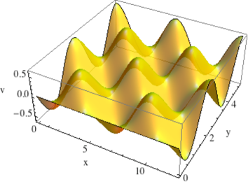
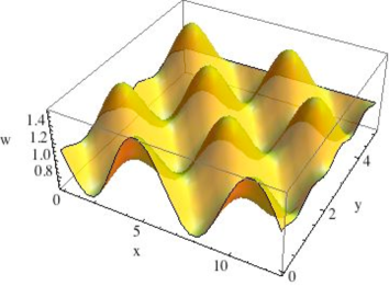
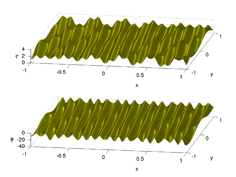
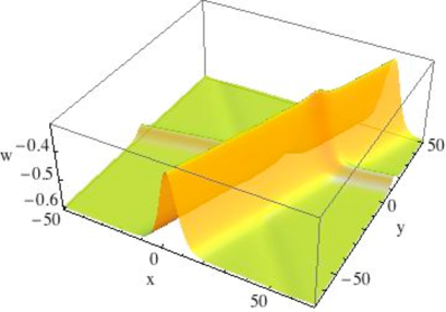
where sn[โ‹…|m]{\rm sn}[\cdot|m] is a Jacobi elliptic function and Kโ€‹(m)๐พ๐‘šK(m) is the complete elliptic integral of the first kind (e.g. [1]), 0<c<10๐‘10<c<1 and e>1๐‘’1e>1, one obtains bounded doubly periodic solutions vโ€‹(x,y,t)=(uy+ut)โ€‹cosโกx๐‘ฃ๐‘ฅ๐‘ฆ๐‘กsubscript๐‘ข๐‘ฆsubscript๐‘ข๐‘ก๐‘ฅv(x,y,t)=(u_{y}+u_{t})\cos x and wโ€‹(x,y,t)=โˆ’sinhโกuโ€‹sinโกx+coshโกu๐‘ค๐‘ฅ๐‘ฆ๐‘ก๐‘ข๐‘ฅ๐‘ขw(x,y,t)=-\sinh u\sin x+\cosh u of the system (5) shown in Fig.ย 1 for c=1/3๐‘13c=1/3 and e=1.1๐‘’1.1e=1.1 (plotted using Mathematica [28]). These solutions remain non-singular for all values of t๐‘กt.

Refer to caption
Refer to caption
Figure 1: Solution (13), (14) to the system (5) for v๐‘ฃv and w๐‘คw at t=0๐‘ก0t=0.

Reduction to the KdV equation. Let vโ€‹(x,y,ฯ„)๐‘ฃ๐‘ฅ๐‘ฆ๐œv(x,y,\tau) be a solution to a pair of commuting flows

vฯ„=(ฯ†2)x,vy=14โ€‹vxโ€‹xโ€‹xโˆ’3โ€‹vโ€‹vx,formulae-sequencesubscript๐‘ฃ๐œsubscriptsuperscript๐œ‘2๐‘ฅsubscript๐‘ฃ๐‘ฆ14subscript๐‘ฃ๐‘ฅ๐‘ฅ๐‘ฅ3๐‘ฃsubscript๐‘ฃ๐‘ฅv_{\tau}=(\varphi^{2})_{x},~{}~{}~{}v_{y}=\frac{1}{4}v_{xxx}-3vv_{x},

where ฯ†๐œ‘\varphi satisfies the system

ฯ†xโ€‹x=2โ€‹vโ€‹ฯ†,ฯ†y=12โ€‹vxโ€‹ฯ†โˆ’vโ€‹ฯ†x.formulae-sequencesubscript๐œ‘๐‘ฅ๐‘ฅ2๐‘ฃ๐œ‘subscript๐œ‘๐‘ฆ12subscript๐‘ฃ๐‘ฅ๐œ‘๐‘ฃsubscript๐œ‘๐‘ฅ\varphi_{xx}=2v\varphi,~{}~{}~{}\varphi_{y}=\frac{1}{2}v_{x}\varphi-v\varphi_{x}.

Notice that the last two equations constitute a Lax pair for the KdV equation (at zero value of the spectral parameter), and the consistency condition vฯ„โ€‹y=vyโ€‹ฯ„subscript๐‘ฃ๐œ๐‘ฆsubscript๐‘ฃ๐‘ฆ๐œv_{\tau y}=v_{y\tau} holds identically modulo the equations for ฯ†๐œ‘\varphi. Setting

wโ€‹(x,y,ฯ„)=โˆ’ฯ†2,๐‘ค๐‘ฅ๐‘ฆ๐œsuperscript๐œ‘2w(x,y,\tau)=-\varphi^{2}, (15)

one can see that vโ€‹(x,y,ฯ„)๐‘ฃ๐‘ฅ๐‘ฆ๐œv(x,y,\tau) and wโ€‹(x,y,ฯ„)๐‘ค๐‘ฅ๐‘ฆ๐œw(x,y,\tau) solve the system (12). Exact non-singular multi-soliton solutions of these equations can be constructed in the form

v=โˆ’d2dโ€‹x2โ€‹lnโกWโ€‹(ฯˆ1,โ€ฆ,ฯˆn),ฯ†=1โˆkiโ€‹Wโ€‹(ฯˆ1,โ€ฆ,ฯˆn, 1)Wโ€‹(ฯˆ1,โ€ฆ,ฯˆn);formulae-sequence๐‘ฃsuperscript๐‘‘2๐‘‘superscript๐‘ฅ2๐‘Šsubscript๐œ“1โ€ฆsubscript๐œ“๐‘›๐œ‘1productsubscript๐‘˜๐‘–๐‘Šsubscript๐œ“1โ€ฆsubscript๐œ“๐‘›1๐‘Šsubscript๐œ“1โ€ฆsubscript๐œ“๐‘›v=-\frac{d^{2}}{dx^{2}}\ln W(\psi_{1},\ ...,\psi_{n}),~{}~{}~{}\varphi=\frac{1}{\prod k_{i}}\frac{W(\psi_{1},\ ...,\psi_{n},\ 1)}{W(\psi_{1},...,\psi_{n})}; (16)

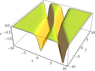
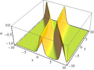
here W๐‘ŠW denotes the Wronskian of n๐‘›n functions ฯˆisubscript๐œ“๐‘–\psi_{i} where ฯˆ2โ€‹jโˆ’1=coshโก(k2โ€‹jโˆ’1โ€‹x+k2โ€‹jโˆ’13โ€‹y+ฯ„/k2โ€‹jโˆ’1)subscript๐œ“2๐‘—1subscript๐‘˜2๐‘—1๐‘ฅsuperscriptsubscript๐‘˜2๐‘—13๐‘ฆ๐œsubscript๐‘˜2๐‘—1\psi_{2j-1}=\cosh(k_{2j-1}x+k_{2j-1}^{3}y+\tau/k_{2j-1}) and ฯˆ2โ€‹j=sinhโก(k2โ€‹jโ€‹x+k2โ€‹j3โ€‹y+ฯ„/k2โ€‹j)subscript๐œ“2๐‘—subscript๐‘˜2๐‘—๐‘ฅsuperscriptsubscript๐‘˜2๐‘—3๐‘ฆ๐œsubscript๐‘˜2๐‘—\psi_{2j}=\sinh(k_{2j}x+k_{2j}^{3}y+\tau/k_{2j}), ki=cโ€‹oโ€‹nโ€‹sโ€‹tsubscript๐‘˜๐‘–๐‘๐‘œ๐‘›๐‘ ๐‘กk_{i}=const satisfying k1<k2<โ€ฆ<kNsubscript๐‘˜1subscript๐‘˜2โ€ฆsubscript๐‘˜๐‘k_{1}<k_{2}<...<k_{N} (e.g., [38]). Taking n=2๐‘›2n=2, k1=1.05subscript๐‘˜11.05k_{1}=1.05, k2=1.2subscript๐‘˜21.2k_{2}=1.2, and setting ฯ„=tโˆ’y๐œ๐‘ก๐‘ฆ\tau=t-y, we obtain a two-soliton solution of the system (5) shown in Fig.ย 2.

Refer to caption
Refer to caption
Figure 2: Solution (15), (16) to the system (5) for v๐‘ฃv and w๐‘คw at t=0๐‘ก0t=0.

Further differential reductions of the system (5) can be obtained from the general approach of [39].

3.3 Reduction to a pair of (1+1)-dimensional linearly degenerate systems

The method of hydrodynamic reductions, originally proposed in [17, 18] in the context of the dispersionless KP hierarchy, was subsequently generalized to a whole class of multi-dimensional quasilinear systems in [13, 14, 15]. We will use the example of system (5) to illustrate the method, see also [33, 40]. Let us seek N๐‘N-phase solutions of the system (5) in the form

v=vโ€‹(R1,โ€ฆ,RN),w=wโ€‹(R1,โ€ฆ,RN)formulae-sequence๐‘ฃ๐‘ฃsuperscript๐‘…1โ€ฆsuperscript๐‘…๐‘๐‘ค๐‘คsuperscript๐‘…1โ€ฆsuperscript๐‘…๐‘v=v(R^{1},...,R^{N}),~{}~{}~{}w=w(R^{1},...,R^{N}) (17)

where the phases (Riemann invariants) Riโ€‹(x,y,t)superscript๐‘…๐‘–๐‘ฅ๐‘ฆ๐‘กR^{i}(x,y,t) satisfy a pair of compatible (1+1)11(1+1)-dimensional systems

Rti=ฮปiโ€‹(R)โ€‹Rxi,Ryi=ฮผiโ€‹(R)โ€‹Rxi.formulae-sequencesubscriptsuperscript๐‘…๐‘–๐‘กsuperscript๐œ†๐‘–๐‘…subscriptsuperscript๐‘…๐‘–๐‘ฅsubscriptsuperscript๐‘…๐‘–๐‘ฆsuperscript๐œ‡๐‘–๐‘…subscriptsuperscript๐‘…๐‘–๐‘ฅR^{i}_{t}=\lambda^{i}(R)R^{i}_{x},~{}~{}~{}R^{i}_{y}=\mu^{i}(R)R^{i}_{x}. (18)

Recall that the commutativity conditions of the flows (18) take the form [42],

โˆ‚jฮปiฮปjโˆ’ฮปi=โˆ‚jฮผiฮผjโˆ’ฮผi,subscript๐‘—superscript๐œ†๐‘–superscript๐œ†๐‘—superscript๐œ†๐‘–subscript๐‘—superscript๐œ‡๐‘–superscript๐œ‡๐‘—superscript๐œ‡๐‘–\frac{\partial_{j}\lambda^{i}}{\lambda^{j}-\lambda^{i}}=\frac{\partial_{j}\mu^{i}}{\mu^{j}-\mu^{i}}, (19)

iโ‰ j,โˆ‚j=โˆ‚/โˆ‚Rjformulae-sequence๐‘–๐‘—subscript๐‘—subscriptsuperscript๐‘…๐‘—i\neq j,~{}\partial_{j}=\partial/\partial_{R^{j}}, no summation. The substitution of the ansatz (17) into (5) implies

โˆ‚iw=โˆ’ฮปiโ€‹โˆ‚iv,ฮผi=โˆ’ฮปiโˆ’vโˆ’wฮปi,formulae-sequencesubscript๐‘–๐‘คsuperscript๐œ†๐‘–subscript๐‘–๐‘ฃsuperscript๐œ‡๐‘–superscript๐œ†๐‘–๐‘ฃ๐‘คsuperscript๐œ†๐‘–\partial_{i}w=-\lambda^{i}\partial_{i}v,~{}~{}~{}\mu^{i}=-\lambda^{i}-v-\frac{w}{\lambda^{i}},

which, taking into account the commutativity condition (19), leads to โˆ‚jlogโกฮปi=โˆ‚jlogโกwsubscript๐‘—superscript๐œ†๐‘–subscript๐‘—๐‘ค\partial_{j}\log\lambda^{i}=\partial_{j}\log w, โˆ‚iโˆ‚jlogโกw=0,โˆ‚iโˆ‚jv=0,iโ‰ jformulae-sequencesubscript๐‘–subscript๐‘—๐‘ค0formulae-sequencesubscript๐‘–subscript๐‘—๐‘ฃ0๐‘–๐‘—\partial_{i}\partial_{j}\log w=0,~{}\partial_{i}\partial_{j}v=0,\ i\neq j. These equations are straightforward to integrate:

v=โˆ‘kฮทkโ€‹(Rk),w=โˆkfkโ€‹(Rk),ฮปi=ฯ†iโ€‹(Ri)โ€‹โˆkfkโ€‹(Rk),formulae-sequence๐‘ฃsubscript๐‘˜superscript๐œ‚๐‘˜superscript๐‘…๐‘˜formulae-sequence๐‘คsubscriptproduct๐‘˜superscript๐‘“๐‘˜superscript๐‘…๐‘˜superscript๐œ†๐‘–superscript๐œ‘๐‘–superscript๐‘…๐‘–subscriptproduct๐‘˜superscript๐‘“๐‘˜superscript๐‘…๐‘˜v=\sum_{k}\eta^{k}(R^{k}),~{}~{}~{}w=\prod_{k}f^{k}(R^{k}),~{}~{}~{}\lambda^{i}=\varphi^{i}(R^{i})\prod_{k}f^{k}(R^{k}),\\

here fiโ€‹(Ri),ฮทiโ€‹(Ri)superscript๐‘“๐‘–superscript๐‘…๐‘–superscript๐œ‚๐‘–superscript๐‘…๐‘–f^{i}(R^{i}),\ \eta^{i}(R^{i}) and ฯ†iโ€‹(Ri)superscript๐œ‘๐‘–superscript๐‘…๐‘–\varphi^{i}(R^{i}) are arbitrary functions of one variable such that (ฮทi)โ€ฒ=โˆ’(fi)โ€ฒ/(fiโ€‹ฯ†i)superscriptsuperscript๐œ‚๐‘–โ€ฒsuperscriptsuperscript๐‘“๐‘–โ€ฒsuperscript๐‘“๐‘–superscript๐œ‘๐‘–(\eta^{i})^{\prime}=-(f^{i})^{\prime}/(f^{i}\varphi^{i}). After a reparametrization Riโ†’fiโ€‹(Ri)โ†’superscript๐‘…๐‘–superscript๐‘“๐‘–superscript๐‘…๐‘–R^{i}\to f^{i}(R^{i}) this simplifies to

v=โˆ‘kฮทkโ€‹(Rk),w=โˆkRk,ฮปi=ฯ†iโ€‹(Ri)โ€‹โˆkRk,(ฮทi)โ€ฒ=โˆ’1/(Riโ€‹ฯ†i).formulae-sequence๐‘ฃsubscript๐‘˜superscript๐œ‚๐‘˜superscript๐‘…๐‘˜formulae-sequence๐‘คsubscriptproduct๐‘˜superscript๐‘…๐‘˜formulae-sequencesuperscript๐œ†๐‘–superscript๐œ‘๐‘–superscript๐‘…๐‘–subscriptproduct๐‘˜superscript๐‘…๐‘˜superscriptsuperscript๐œ‚๐‘–โ€ฒ1superscript๐‘…๐‘–superscript๐œ‘๐‘–v=\sum_{k}\eta^{k}(R^{k}),~{}~{}~{}w=\prod_{k}R^{k},~{}~{}~{}\lambda^{i}=\varphi^{i}(R^{i})\prod_{k}R^{k},~{}~{}~{}(\eta^{i})^{\prime}=-1/(R^{i}\varphi^{i}).

From now on we fix a particular choice ฯ†iโ€‹(Ri)=1/Risuperscript๐œ‘๐‘–superscript๐‘…๐‘–1superscript๐‘…๐‘–\varphi^{i}(R^{i})=1/R^{i} under which both systems in (18) become linearly degenerate:

Rti=(โˆkโ‰ iRk)โ€‹Rxi,Ryi=(โˆ‘kโ‰ iRkโˆ’โˆkโ‰ iRk)โ€‹Rxi.formulae-sequencesubscriptsuperscript๐‘…๐‘–๐‘กsubscriptproduct๐‘˜๐‘–superscript๐‘…๐‘˜subscriptsuperscript๐‘…๐‘–๐‘ฅsubscriptsuperscript๐‘…๐‘–๐‘ฆsubscript๐‘˜๐‘–superscript๐‘…๐‘˜subscriptproduct๐‘˜๐‘–superscript๐‘…๐‘˜subscriptsuperscript๐‘…๐‘–๐‘ฅR^{i}_{t}=(\prod_{k\neq i}R^{k})\ R^{i}_{x},~{}~{}~{}~{}~{}R^{i}_{y}=(\sum_{k\neq i}R^{k}-\prod_{k\neq i}R^{k})\ R^{i}_{x}. (20)

Once a solution to equations (20) is known, the variables v๐‘ฃv and w๐‘คw can be reconstructed by the formulae

v=โˆ’โˆ‘kRk,w=โˆkRk.formulae-sequence๐‘ฃsubscript๐‘˜superscript๐‘…๐‘˜๐‘คsubscriptproduct๐‘˜superscript๐‘…๐‘˜v=-\sum_{k}R^{k},~{}~{}~{}w=\prod_{k}R^{k}.

Thus, the (2+1)21(2+1)-dimensional system (5) is decoupled into a pair of (1+1)11(1+1)-dimensional linearly degenerate systems (20) with an arbitrarily large number of dependent variables N๐‘N. Since the gradient catastrophe for one-dimensional linearly degenerate hyperbolic systems does not occur [35, 36, 23, 37], generic solutions arising from this construction will not break down in finite time. The general solution of Eqs. (20) can be represented in the following parametric form,

โˆซR1ฮพNโˆ’1โ€‹dโ€‹ฮพf1โ€‹(ฮพ)+โ‹ฏ+โˆซRNฮพNโˆ’1โ€‹dโ€‹ฮพfNโ€‹(ฮพ)=x,โˆซR1ฮพNโˆ’2โ€‹dโ€‹ฮพf1โ€‹(ฮพ)+โ‹ฏ+โˆซRNฮพNโˆ’2โ€‹dโ€‹ฮพfNโ€‹(ฮพ)=โˆ’y,โˆซR1ฮพkโ€‹dโ€‹ฮพf1โ€‹(ฮพ)+โ‹ฏ+โˆซRNฮพkโ€‹dโ€‹ฮพfNโ€‹(ฮพ)=0,k=1,2,โ€ฆ,Nโˆ’3,โˆซR1dโ€‹ฮพf1โ€‹(ฮพ)+โ‹ฏ+โˆซRNdโ€‹ฮพfNโ€‹(ฮพ)=(โˆ’1)Nโ€‹(yโˆ’t),superscriptsuperscript๐‘…1absentsuperscript๐œ‰๐‘1๐‘‘๐œ‰subscript๐‘“1๐œ‰limit-fromโ‹ฏsuperscriptsuperscript๐‘…๐‘superscript๐œ‰๐‘1๐‘‘๐œ‰subscript๐‘“๐‘๐œ‰๐‘ฅmissing-subexpressionsuperscriptsuperscript๐‘…1absentsuperscript๐œ‰๐‘2๐‘‘๐œ‰subscript๐‘“1๐œ‰limit-fromโ‹ฏsuperscriptsuperscript๐‘…๐‘superscript๐œ‰๐‘2๐‘‘๐œ‰subscript๐‘“๐‘๐œ‰๐‘ฆmissing-subexpressionformulae-sequencesuperscriptsuperscript๐‘…1absentsuperscript๐œ‰๐‘˜๐‘‘๐œ‰subscript๐‘“1๐œ‰limit-fromโ‹ฏsuperscriptsuperscript๐‘…๐‘superscript๐œ‰๐‘˜๐‘‘๐œ‰subscript๐‘“๐‘๐œ‰0๐‘˜12โ€ฆ๐‘3missing-subexpressionsuperscriptsuperscript๐‘…1absent๐‘‘๐œ‰subscript๐‘“1๐œ‰limit-fromโ‹ฏsuperscriptsuperscript๐‘…๐‘๐‘‘๐œ‰subscript๐‘“๐‘๐œ‰superscript1๐‘๐‘ฆ๐‘ก\begin{array}[]{c}\stackrel{{\scriptstyle R^{1}}}{{\int}}\frac{\xi^{N-1}d\xi}{f_{1}(\xi)}+\dots+\stackrel{{\scriptstyle R^{N}}}{{\int}}\frac{\xi^{N-1}d\xi}{f_{N}(\xi)}=x,\\ \\ \stackrel{{\scriptstyle R^{1}}}{{\int}}\frac{\xi^{N-2}d\xi}{f_{1}(\xi)}+\dots+\stackrel{{\scriptstyle R^{N}}}{{\int}}\frac{\xi^{N-2}d\xi}{f_{N}(\xi)}=-y,\\ \\ \stackrel{{\scriptstyle R^{1}}}{{\int}}\frac{\xi^{k}d\xi}{f_{1}(\xi)}+\dots+\stackrel{{\scriptstyle R^{N}}}{{\int}}\frac{\xi^{k}d\xi}{f_{N}(\xi)}=0,~{}~{}~{}k=1,2,...,N-3,\\ \\ \stackrel{{\scriptstyle R^{1}}}{{\int}}\frac{d\xi}{f_{1}(\xi)}+\dots+\stackrel{{\scriptstyle R^{N}}}{{\int}}\frac{d\xi}{f_{N}(\xi)}=(-1)^{N}(y-t),\end{array} (21)

see [12], where fiโ€‹(ฮพ)subscript๐‘“๐‘–๐œ‰f_{i}(\xi) are N๐‘N arbitrary functions of one variable. In the next subsections we utilize this representation to construct particular solutions of system (5) representing various multiple-wave interactions.

3.3.1 Reduction to the Jacobi inversion problem

With the choice fiโ€‹(ฮพ)=P2โ€‹N+1โ€‹(ฮพ)subscript๐‘“๐‘–๐œ‰subscript๐‘ƒ2๐‘1๐œ‰f_{i}(\xi)=\sqrt{P_{2N+1}(\xi)}, i=1,โ€ฆ,N,๐‘–1โ€ฆ๐‘i=1,\ldots,N, where P2โ€‹N+1โ€‹(ฮพ)subscript๐‘ƒ2๐‘1๐œ‰P_{2N+1}(\xi) is a polynomial of degree 2โ€‹N+12๐‘12N+1 in ฮพ๐œ‰\xi, Eqs. (21) reduce to the Jacobi inversion problem which can solved using multi-dimensional theta functions.

The equation ฮผ2=ฮพโ€‹โˆi=12โ€‹N(ฮพโˆ’ฮปi)superscript๐œ‡2๐œ‰superscriptsubscriptproduct๐‘–12๐‘๐œ‰subscript๐œ†๐‘–\mu^{2}=\xi\prod_{i=1}^{2N}(\xi-\lambda_{i}) with ฮปiโˆˆโ„subscript๐œ†๐‘–โ„\lambda_{i}\in\mathbb{R}, i=1,โ€ฆ,2โ€‹N๐‘–1โ€ฆ2๐‘i=1,\ldots,2N, ฮปiโ‰ ฮปjsubscript๐œ†๐‘–subscript๐œ†๐‘—\lambda_{i}\neq\lambda_{j} for iโ‰ j๐‘–๐‘—i\neq j and ฮปiโ‰ 0subscript๐œ†๐‘–0\lambda_{i}\neq 0 defines a hyperelliptic Riemann surface โ„’โ„’\mathcal{L} of genus N๐‘N with simple branch points at the ฮปisubscript๐œ†๐‘–\lambda_{i}, 0 and at infinity. In addition we choose โˆ‘i=1Nฮปi=0superscriptsubscript๐‘–1๐‘subscript๐œ†๐‘–0\sum_{i=1}^{N}\lambda_{i}=0111More general hyperelliptic Riemann surfaces can be used in this context, but since we only want to illustrate this approach, we took this choice leading to simple formulae. With this choice, v๐‘ฃv will be a solution to the KdV equation. We order the branch points in a way that ฮป1<ฮป2<โ€ฆ<0<โ€ฆ<ฮป2โ€‹Nsubscript๐œ†1subscript๐œ†2โ€ฆ0โ€ฆsubscript๐œ†2๐‘\lambda_{1}<\lambda_{2}<\ldots<0<\ldots<\lambda_{2N}. The differentials

ฮทk=ฮพkโˆ’1โ€‹dโ€‹ฮพฮผ,k=1,โ€ฆ,N,formulae-sequencesubscript๐œ‚๐‘˜superscript๐œ‰๐‘˜1๐‘‘๐œ‰๐œ‡๐‘˜1โ€ฆ๐‘\eta_{k}=\frac{\xi^{k-1}d\xi}{\mu},\quad k=1,\ldots,N,

form a basis for the holomorphic one-forms on โ„’โ„’\mathcal{L}. On this surface we introduce a basis of the homology, where the a๐‘Ža-cycles are in the upper sheet each of them encircling exactly one of the cuts between [ฮป1,ฮป2]subscript๐œ†1subscript๐œ†2[\lambda_{1},\lambda_{2}], [ฮป3,ฮป4]subscript๐œ†3subscript๐œ†4[\lambda_{3},\lambda_{4}],โ€ฆ,[ฮป2โ€‹Nโˆ’2,ฮป2โ€‹Nโˆ’1]subscript๐œ†2๐‘2subscript๐œ†2๐‘1[\lambda_{2N-2},\lambda_{2N-1}]; all b๐‘b-cycles start at the cut [ฮป2โ€‹N,โˆž]subscript๐œ†2๐‘[\lambda_{2N},\infty], and each of them intersects exactly one a๐‘Ža-cycle such that aiโ‹…bj=ฮดiโ€‹jโ‹…subscript๐‘Ž๐‘–subscript๐‘๐‘—subscript๐›ฟ๐‘–๐‘—a_{i}\cdot b_{j}=\delta_{ij}. A normalized basis of holomorphic differentials ฯ‰isubscript๐œ”๐‘–\omega_{i}, i=1,โ€ฆ,Nโˆ’1๐‘–1โ€ฆ๐‘1i=1,\ldots,N-1 is given by

ฯ‰i=โˆ‘j=1Nciโ€‹jโ€‹ฮทj,i=1,โ€ฆ,N,formulae-sequencesubscript๐œ”๐‘–superscriptsubscript๐‘—1๐‘subscript๐‘๐‘–๐‘—subscript๐œ‚๐‘—๐‘–1โ€ฆ๐‘\omega_{i}=\sum_{j=1}^{N}c_{ij}\eta_{j},\quad i=1,\ldots,N,

where the ciโ€‹jsubscript๐‘๐‘–๐‘—c_{ij} are fixed by the normalization condition

โˆซaiฯ‰j=2โ€‹ฯ€โ€‹iโ€‹ฮดiโ€‹j,i,j=1,โ€ฆ,N.formulae-sequencesubscriptsubscript๐‘Ž๐‘–subscript๐œ”๐‘—2๐œ‹isubscript๐›ฟ๐‘–๐‘—๐‘–๐‘—1โ€ฆ๐‘\int_{a_{i}}\omega_{j}=2\pi\mathrm{i}\delta_{ij},\quad i,j=1,\ldots,N.

With this normalization the matrix

๐”นiโ€‹j=โˆซbiฯ‰j,i,j=1,โ€ฆ,N,formulae-sequencesubscript๐”น๐‘–๐‘—subscriptsubscript๐‘๐‘–subscript๐œ”๐‘—๐‘–๐‘—1โ€ฆ๐‘\mathbb{B}_{ij}=\int_{b_{i}}\omega_{j},\quad i,j=1,\ldots,N,

is a Riemann matrix, i.e., it is symmetric and has a negative definite real part (see for instance [2]). Therefore the theta function with half integer characteristics [ฮฑ]=[ฮฑโ€ฒ;ฮฑโ€ฒโ€ฒ]โˆˆโ„2โ€‹Ndelimited-[]๐›ผsuperscript๐›ผโ€ฒsuperscript๐›ผโ€ฒโ€ฒsuperscriptโ„2๐‘[\alpha]=[\alpha^{\prime};\alpha^{\prime\prime}]\in\mathbb{R}^{2N} defined by

ฮ˜โ€‹[ฮฑ]โ€‹(๐ฑ|๐”น)=โˆ‘๐งโˆˆโ„คNexpโก(12โ€‹โŸจ๐ง+ฮฑโ€ฒ,๐”นโ€‹(๐ง+ฮฑโ€ฒ)โŸฉ+โŸจ๐ง+ฮฑโ€ฒ,๐ฑ+2โ€‹ฯ€โ€‹iโ€‹ฮฑโ€ฒโ€ฒโŸฉ),ฮ˜delimited-[]๐›ผconditional๐ฑ๐”นsubscript๐งsuperscriptโ„ค๐‘12๐งsuperscript๐›ผโ€ฒ๐”น๐งsuperscript๐›ผโ€ฒ๐งsuperscript๐›ผโ€ฒ๐ฑ2๐œ‹isuperscript๐›ผโ€ฒโ€ฒ\Theta[\alpha](\mathbf{x}|\mathbb{B})=\sum_{\mathbf{n}\in\mathbb{Z}^{N}}\exp\left(\frac{1}{2}\langle\mathbf{n+\alpha^{\prime}},\mathbb{B}(\mathbf{n+\alpha^{\prime}})\rangle+\langle\mathbf{n+\alpha^{\prime}},\mathbf{x}+2\pi\mathrm{i}\alpha^{\prime\prime}\rangle\right),

where the angular brackets denote the Euclidean scalar product, is an entire function for all ๐ณโˆˆโ„‚N.๐ณsuperscriptโ„‚๐‘\mathbf{z}\in\mathbb{C}^{N}.

With this setting the Jacobi inversion problem following from (21) can be written in the form

โˆ‘j=1NโˆซRjฯ‰i=ciโ€‹Nxโˆ’ciโ€‹(Nโˆ’1)y+ciโ€‹1(โˆ’1)N(yโˆ’t)=:zi.\sum_{j=1}^{N}\int^{R^{j}}\omega_{i}=c_{iN}x-c_{i(N-1)}y+c_{i1}(-1)^{N}(y-t)=:z_{i}.

Notice that an arbitrary constant can be added to each zisubscript๐‘ง๐‘–z_{i} reflecting the freedom to choose a lower limit of the integrals on the left-hand side. Formulae for the symmetric functions โˆ‘j=1NRjsuperscriptsubscript๐‘—1๐‘superscript๐‘…๐‘—\sum_{j=1}^{N}R^{j} and โˆj=1NRjsuperscriptsubscriptproduct๐‘—1๐‘superscript๐‘…๐‘—\prod_{j=1}^{N}R^{j} in terms of theta functions can be found for instance in [2]: the former appears in the hyperelliptic solutions to the KdV equation, the latter (as a logarithm) in the hyperelliptic solutions of the sine-Gordon equation, which is related to the sinh-Gordon equation by the transformation uโ†’iโ€‹uโ†’๐‘ขi๐‘ขu\to\mathrm{i}u. Thus not surprisingly both equations which appear as reductions of the studied systems also play a role in the context of hyperelliptic solutions. We have

v=โˆ’โˆ‘i=1NRi=โˆ’(c+โˆ‚xโ€‹xlnโกฮ˜โ€‹[ฮฑ]โ€‹(z)),w=โˆi=1NRi=d+โˆ‚xโ€‹tlnโกฮ˜โ€‹[ฮฑ]โ€‹(z),formulae-sequence๐‘ฃsuperscriptsubscript๐‘–1๐‘superscript๐‘…๐‘–๐‘subscript๐‘ฅ๐‘ฅฮ˜delimited-[]๐›ผ๐‘ง๐‘คsuperscriptsubscriptproduct๐‘–1๐‘superscript๐‘…๐‘–๐‘‘subscript๐‘ฅ๐‘กฮ˜delimited-[]๐›ผ๐‘งv=-\sum_{i=1}^{N}R^{i}=-(c+\partial_{xx}\ln\Theta[\alpha](z)),\quad w=\prod_{i=1}^{N}R^{i}=d+\partial_{xt}\ln\Theta[\alpha](z), (22)

where the arbitrary non-singular constant characteristic reflects the possibility to change ๐ณ๐ณ\mathbf{z} by an arbitrary constant, and where c๐‘c and d๐‘‘d are constants with respect to the physical coordinates,

c=12โ€‹ฯ€โ€‹iโ€‹โˆ‘i=1Nciโ€‹Nโ€‹โˆซaiฮพgโ€‹dโ€‹ฮพฮผ,d=โˆ‚xโ€‹tlnโกฮ˜โ€‹[ฮฑโˆ—]โ€‹(โˆซ0โˆžฯ‰),formulae-sequence๐‘12๐œ‹isuperscriptsubscript๐‘–1๐‘subscript๐‘๐‘–๐‘subscriptsubscript๐‘Ž๐‘–superscript๐œ‰๐‘”๐‘‘๐œ‰๐œ‡๐‘‘subscript๐‘ฅ๐‘กฮ˜delimited-[]superscript๐›ผsuperscriptsubscript0๐œ”c=\frac{1}{2\pi\mathrm{i}}\sum_{i=1}^{N}c_{iN}\int_{a_{i}}\frac{\xi^{g}d\xi}{\mu},\quad d=\partial_{xt}\ln\Theta[\alpha^{*}]\left(\int_{0}^{\infty}\omega\right),

where [ฮฑโˆ—]delimited-[]superscript๐›ผ[\alpha^{*}] is an arbitrary odd half integer characteristic. It can be seen that vt+wx=0subscript๐‘ฃ๐‘กsubscript๐‘ค๐‘ฅ0v_{t}+w_{x}=0 by construction. The validity of the second equation in (12) is checked by applying derivatives to the theta functions and computing these numerically. Since this relation is not implemented in the code, its validity provides a strong test on the quality of the numerics. The code typically satisfies this test to the order of machine precision. We use the code [16] developed for hyperelliptic solutions to KdV, Kadomtsev-Petviashvili and other equations. In Fig.ย 3 one can see a typical genus 3 solution.
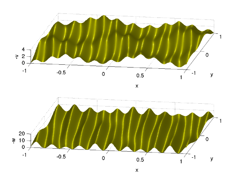
Refer to caption
Figure 3: Solutions v๐‘ฃv and w๐‘คw (22) for N=3๐‘3N=3 on the surface with branch points [โˆ’3โˆ’ฯต,โˆ’3,โˆ’ฯต,0,1,1+2โ€‹ฯต,4]3italic-ฯต3italic-ฯต0112italic-ฯต4[-3-\epsilon,-3,-\epsilon,0,1,1+2\epsilon,4] for ฯต=1italic-ฯต1\epsilon=1 at t=0๐‘ก0t=0. The characteristics of the theta function are chosen to be ฮฑiโ€ฒ=1/2superscriptsubscript๐›ผ๐‘–โ€ฒ12\alpha_{i}^{\prime}=1/2 and ฮฑiโ€ฒโ€ฒ=0superscriptsubscript๐›ผ๐‘–โ€ฒโ€ฒ0\alpha_{i}^{\prime\prime}=0 for i=1,2,3๐‘–123i=1,2,3.

As already mentioned, v๐‘ฃv solves the KdV equation in y๐‘ฆy and x๐‘ฅx, the time t๐‘กt playing just the role of a parameter here. In Fig.ย 4, the same situation as in Fig.ย 3 can be seen for t=0.1๐‘ก0.1t=0.1 thus illustrating the time evolution of the pattern.
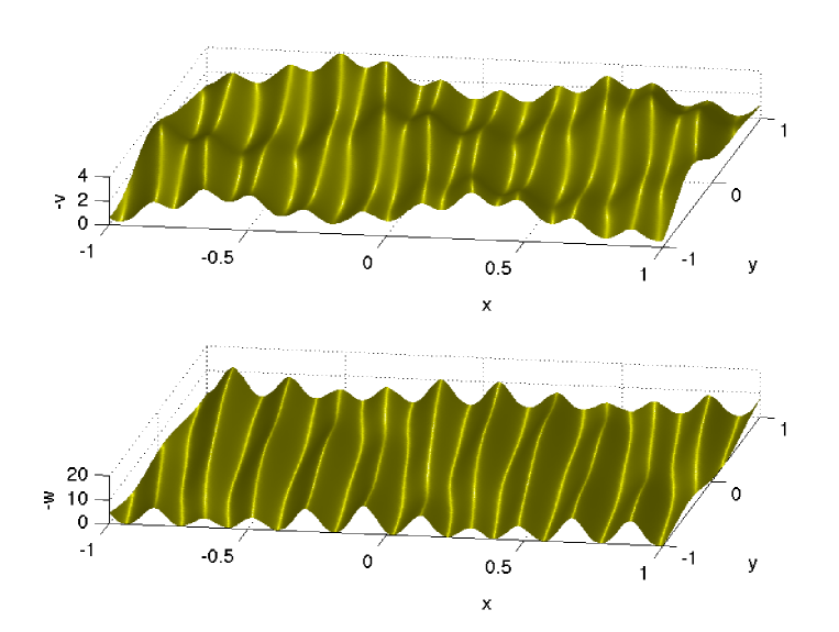
Refer to caption
Figure 4: Solutions v๐‘ฃv and w๐‘คw (22) for N=3๐‘3N=3 on the surface with branch points [โˆ’3โˆ’ฯต,โˆ’3,โˆ’ฯต,0,1,1+2โ€‹ฯต,4]3italic-ฯต3italic-ฯต0112italic-ฯต4[-3-\epsilon,-3,-\epsilon,0,1,1+2\epsilon,4] for ฯต=1italic-ฯต1\epsilon=1 at t=0.1๐‘ก0.1t=0.1. The characteristics of the theta function are chosen to be ฮฑiโ€ฒ=1/2superscriptsubscript๐›ผ๐‘–โ€ฒ12\alpha_{i}^{\prime}=1/2 and ฮฑiโ€ฒโ€ฒ=0superscriptsubscript๐›ผ๐‘–โ€ฒโ€ฒ0\alpha_{i}^{\prime\prime}=0 for i=1,2,3๐‘–123i=1,2,3.

If the ฯตitalic-ฯต\epsilon in Fig.ย 3 tends to 0, the surface degenerates which leads to the solitonic limit of the KdV solution v๐‘ฃv. This can be seen in Fig.ย 5 where a 3-soliton solution to KdV appears. The characteristic phase shift at the point of collision between the solitons can be clearly recognized.
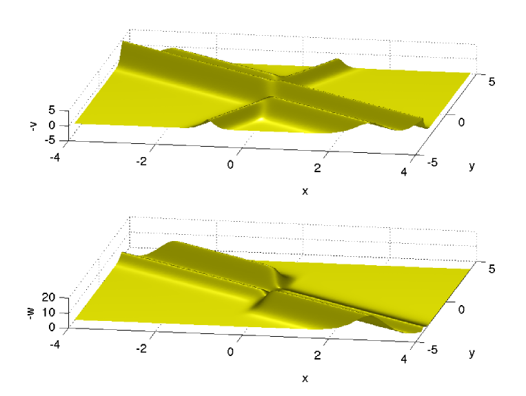
Refer to caption
Figure 5: Solutions v๐‘ฃv and w๐‘คw (22) for N=3๐‘3N=3 on the surface with branch points [โˆ’3โˆ’ฯต,โˆ’3,โˆ’ฯต,0,1,1+2โ€‹ฯต,4]3italic-ฯต3italic-ฯต0112italic-ฯต4[-3-\epsilon,-3,-\epsilon,0,1,1+2\epsilon,4] for ฯต=10โˆ’14italic-ฯตsuperscript1014\epsilon=10^{-14} at t=0๐‘ก0t=0. The characteristics of the theta function are chosen to be ฮฑiโ€ฒ=1/2superscriptsubscript๐›ผ๐‘–โ€ฒ12\alpha_{i}^{\prime}=1/2 and ฮฑiโ€ฒโ€ฒ=0superscriptsubscript๐›ผ๐‘–โ€ฒโ€ฒ0\alpha_{i}^{\prime\prime}=0 for i=1,2,3๐‘–123i=1,2,3.

In this sense the solutions on a non-degenerate surface can be loosely interpreted as an infinite train of 3-solitons. Going to higher genus, one obtains N๐‘N-phase solutions which show with increasing N๐‘N more and more structure, as can be seen for instance in Fig.ย 6.

Refer to caption
Figure 6: Solutions v๐‘ฃv and w๐‘คw (22) for N=4๐‘4N=4 on the surface with branch points [โˆ’4,โˆ’3,โˆ’2,โˆ’1,0,1,2,3,4]432101234[-4,-3,-2,-1,0,1,2,3,4] at t=0๐‘ก0t=0. The characteristics of the theta function are chosen to be ฮฑiโ€ฒ=1/2superscriptsubscript๐›ผ๐‘–โ€ฒ12\alpha_{i}^{\prime}=1/2 and ฮฑiโ€ฒโ€ฒ=0superscriptsubscript๐›ผ๐‘–โ€ฒโ€ฒ0\alpha_{i}^{\prime\prime}=0 for i=1,2,3,4๐‘–1234i=1,2,3,4.

3.3.2 Parametric plots of 3-wave interactions

In the case N=3๐‘3N=3 Eqs. (20) reduce to

Rt1=R2โ€‹R3โ€‹Rx1,Rt2=R1โ€‹R3โ€‹Rx2,Rt3=R1โ€‹R2โ€‹Rx3formulae-sequencesubscriptsuperscript๐‘…1๐‘กsuperscript๐‘…2superscript๐‘…3subscriptsuperscript๐‘…1๐‘ฅformulae-sequencesubscriptsuperscript๐‘…2๐‘กsuperscript๐‘…1superscript๐‘…3subscriptsuperscript๐‘…2๐‘ฅsubscriptsuperscript๐‘…3๐‘กsuperscript๐‘…1superscript๐‘…2subscriptsuperscript๐‘…3๐‘ฅR^{1}_{t}=R^{2}R^{3}\ R^{1}_{x},~{}~{}~{}R^{2}_{t}=R^{1}R^{3}\ R^{2}_{x},~{}~{}~{}R^{3}_{t}=R^{1}R^{2}\ R^{3}_{x} (23)

and

Ry1=(R2+R3โˆ’R2โ€‹R3)โ€‹Rx1,Ry2=(R1+R3โˆ’R1โ€‹R3)โ€‹Rx2,Ry3=(R1+R2โˆ’R1โ€‹R2)โ€‹Rx3,formulae-sequencesubscriptsuperscript๐‘…1๐‘ฆsuperscript๐‘…2superscript๐‘…3superscript๐‘…2superscript๐‘…3subscriptsuperscript๐‘…1๐‘ฅformulae-sequencesubscriptsuperscript๐‘…2๐‘ฆsuperscript๐‘…1superscript๐‘…3superscript๐‘…1superscript๐‘…3subscriptsuperscript๐‘…2๐‘ฅsubscriptsuperscript๐‘…3๐‘ฆsuperscript๐‘…1superscript๐‘…2superscript๐‘…1superscript๐‘…2subscriptsuperscript๐‘…3๐‘ฅR^{1}_{y}=(R^{2}+R^{3}-R^{2}R^{3})\ R^{1}_{x},~{}~{}~{}R^{2}_{y}=(R^{1}+R^{3}-R^{1}R^{3})\ R^{2}_{x},~{}~{}~{}R^{3}_{y}=(R^{1}+R^{2}-R^{1}R^{2})\ R^{3}_{x}, (24)

respectively. The formulae (21) simplify to

โˆซR1ฮพ2โ€‹dโ€‹ฮพfโ€‹(ฮพ)+โˆซR2ฮพ2โ€‹dโ€‹ฮพgโ€‹(ฮพ)+โˆซR3ฮพ2โ€‹dโ€‹ฮพhโ€‹(ฮพ)=x,โˆซR1ฮพโ€‹dโ€‹ฮพfโ€‹(ฮพ)+โˆซR2ฮพโ€‹dโ€‹ฮพgโ€‹(ฮพ)+โˆซR3ฮพโ€‹dโ€‹ฮพhโ€‹(ฮพ)=โˆ’y,โˆซR1dโ€‹ฮพfโ€‹(ฮพ)+โˆซR2dโ€‹ฮพgโ€‹(ฮพ)+โˆซR3dโ€‹ฮพhโ€‹(ฮพ)=tโˆ’y,superscriptsuperscript๐‘…1absentlimit-fromsuperscript๐œ‰2๐‘‘๐œ‰๐‘“๐œ‰superscriptsuperscript๐‘…2limit-fromsuperscript๐œ‰2๐‘‘๐œ‰๐‘”๐œ‰superscriptsuperscript๐‘…3superscript๐œ‰2๐‘‘๐œ‰โ„Ž๐œ‰๐‘ฅmissing-subexpressionsuperscriptsuperscript๐‘…1absentlimit-from๐œ‰๐‘‘๐œ‰๐‘“๐œ‰superscriptsuperscript๐‘…2limit-from๐œ‰๐‘‘๐œ‰๐‘”๐œ‰superscriptsuperscript๐‘…3๐œ‰๐‘‘๐œ‰โ„Ž๐œ‰๐‘ฆmissing-subexpressionsuperscriptsuperscript๐‘…1absentlimit-from๐‘‘๐œ‰๐‘“๐œ‰superscriptsuperscript๐‘…2limit-from๐‘‘๐œ‰๐‘”๐œ‰superscriptsuperscript๐‘…3๐‘‘๐œ‰โ„Ž๐œ‰๐‘ก๐‘ฆ\begin{array}[]{c}\stackrel{{\scriptstyle R^{1}}}{{\int}}\frac{\xi^{2}d\xi}{f(\xi)}+\stackrel{{\scriptstyle R^{2}}}{{\int}}\frac{\xi^{2}d\xi}{g(\xi)}+\stackrel{{\scriptstyle R^{3}}}{{\int}}\frac{\xi^{2}d\xi}{h(\xi)}=x,\\ \\ \stackrel{{\scriptstyle R^{1}}}{{\int}}\frac{\xi d\xi}{f(\xi)}+\stackrel{{\scriptstyle R^{2}}}{{\int}}\frac{\xi d\xi}{g(\xi)}+\stackrel{{\scriptstyle R^{3}}}{{\int}}\frac{\xi d\xi}{h(\xi)}=-y,\\ \\ \stackrel{{\scriptstyle R^{1}}}{{\int}}\frac{d\xi}{f(\xi)}+\stackrel{{\scriptstyle R^{2}}}{{\int}}\frac{d\xi}{g(\xi)}+\stackrel{{\scriptstyle R^{3}}}{{\int}}\frac{d\xi}{h(\xi)}=t-y,\end{array} (25)

where f,g,h๐‘“๐‘”โ„Žf,g,h are arbitrary functions. For our purposes, it will be more convenient to work with an equivalent parametric representation of the general solution of (23)โ€“(24), namely,

R1=Fโ€‹(a),R2=Gโ€‹(b),R3=Hโ€‹(c),formulae-sequencesuperscript๐‘…1๐น๐‘Žformulae-sequencesuperscript๐‘…2๐บ๐‘superscript๐‘…3๐ป๐‘R^{1}=F(a),~{}~{}~{}R^{2}=G(b),~{}~{}~{}R^{3}=H(c),

where a,b,c๐‘Ž๐‘๐‘a,b,c are functions of x,y,t๐‘ฅ๐‘ฆ๐‘กx,y,t defined implicitly via

โˆซF2โ€‹(a)Fโ€‹(a)โˆ’1โ€‹๐‘‘a+โˆซG2โ€‹(b)Gโ€‹(b)โˆ’1โ€‹๐‘‘b+โˆซH2โ€‹(c)Hโ€‹(c)โˆ’1โ€‹๐‘‘c=x,โˆซFโ€‹(a)Fโ€‹(a)โˆ’1โ€‹๐‘‘a+โˆซGโ€‹(b)Gโ€‹(b)โˆ’1โ€‹๐‘‘b+โˆซHโ€‹(c)Hโ€‹(c)โˆ’1โ€‹๐‘‘c=โˆ’y,a+b+c=โˆ’t;superscript๐น2๐‘Ž๐น๐‘Ž1differential-d๐‘Žsuperscript๐บ2๐‘๐บ๐‘1differential-d๐‘superscript๐ป2๐‘๐ป๐‘1differential-d๐‘๐‘ฅmissing-subexpression๐น๐‘Ž๐น๐‘Ž1differential-d๐‘Ž๐บ๐‘๐บ๐‘1differential-d๐‘๐ป๐‘๐ป๐‘1differential-d๐‘๐‘ฆmissing-subexpression๐‘Ž๐‘๐‘๐‘ก\begin{array}[]{c}\int\frac{F^{2}(a)}{F(a)-1}da+\int\frac{G^{2}(b)}{G(b)-1}db+\int\frac{H^{2}(c)}{H(c)-1}dc=x,\\ \\ \int\frac{F(a)}{F(a)-1}da+\int\frac{G(b)}{G(b)-1}db+\int\frac{H(c)}{H(c)-1}dc=-y,\\ \\ a+b+c=-t;\end{array} (26)

here F,G,H๐น๐บ๐ปF,G,H are three arbitrary functions, and all integrals are understood as indefinite. The corresponding solution of (5) is given by the formulae

v=โˆ’Fโ€‹(a)โˆ’Gโ€‹(b)โˆ’Hโ€‹(c),w=Fโ€‹(a)โ€‹Gโ€‹(b)โ€‹Hโ€‹(c).formulae-sequence๐‘ฃ๐น๐‘Ž๐บ๐‘๐ป๐‘๐‘ค๐น๐‘Ž๐บ๐‘๐ป๐‘v=-F(a)-G(b)-H(c),~{}~{}~{}w=F(a)G(b)H(c). (27)

Relations (26) can be derived from (25) by setting

R1=Fโ€‹(a),R2=Gโ€‹(b),R3=Hโ€‹(c)formulae-sequencesuperscript๐‘…1๐น๐‘Žformulae-sequencesuperscript๐‘…2๐บ๐‘superscript๐‘…3๐ป๐‘R^{1}=F(a),~{}~{}R^{2}=G(b),~{}~{}R^{3}=H(c)

and

โˆซR1(ฮพโˆ’1)โ€‹dโ€‹ฮพfโ€‹(ฮพ)=a,โˆซR2(ฮพโˆ’1)โ€‹dโ€‹ฮพgโ€‹(ฮพ)=b,โˆซR3(ฮพโˆ’1)โ€‹dโ€‹ฮพhโ€‹(ฮพ)=c,\stackrel{{\scriptstyle R^{1}}}{{\int}}\frac{(\xi-1)d\xi}{f(\xi)}=a,~{}~{}~{}\stackrel{{\scriptstyle R^{2}}}{{\int}}\frac{(\xi-1)d\xi}{g(\xi)}=b,~{}~{}~{}\stackrel{{\scriptstyle R^{3}}}{{\int}}\frac{(\xi-1)d\xi}{h(\xi)}=c,

respectively. Let us choose, for instance, three soliton-like profiles

Fโ€‹(a)=ฮฑโˆ’ฯตcosh2โกฮผโ€‹a,Gโ€‹(b)=ฮฒโˆ’ฯตcosh2โกฮผโ€‹b,Hโ€‹(c)=ฮณโˆ’ฯตcosh2โกฮผโ€‹c,formulae-sequence๐น๐‘Ž๐›ผitalic-ฯตsuperscript2๐œ‡๐‘Žformulae-sequence๐บ๐‘๐›ฝitalic-ฯตsuperscript2๐œ‡๐‘๐ป๐‘๐›พitalic-ฯตsuperscript2๐œ‡๐‘F(a)=\alpha-\frac{\epsilon}{\cosh^{2}\mu a},~{}~{}~{}G(b)=\beta-\frac{\epsilon}{\cosh^{2}\mu b},~{}~{}~{}H(c)=\gamma-\frac{\epsilon}{\cosh^{2}\mu c}, (28)

where ฮฑ,ฮฒ,ฮณ๐›ผ๐›ฝ๐›พ\alpha,\beta,\gamma are distinct constants and ฯตitalic-ฯต\epsilon is a small parameter. In this case equations (26) take the form

ฮฑ2โ€‹aฮฑโˆ’1+ฮฒ2โ€‹bฮฒโˆ’1+ฮณ2โ€‹cฮณโˆ’1+ฯตโ€‹(โ€ฆ)=x,ฮฑโ€‹aฮฑโˆ’1+ฮฒโ€‹bฮฒโˆ’1+ฮณโ€‹cฮณโˆ’1+ฯตโ€‹(โ€ฆ)=โˆ’y,a+b+c=โˆ’t,formulae-sequencesuperscript๐›ผ2๐‘Ž๐›ผ1superscript๐›ฝ2๐‘๐›ฝ1superscript๐›พ2๐‘๐›พ1italic-ฯตโ€ฆ๐‘ฅformulae-sequence๐›ผ๐‘Ž๐›ผ1๐›ฝ๐‘๐›ฝ1๐›พ๐‘๐›พ1italic-ฯตโ€ฆ๐‘ฆ๐‘Ž๐‘๐‘๐‘ก\frac{\alpha^{2}a}{\alpha-1}+\frac{\beta^{2}b}{\beta-1}+\frac{\gamma^{2}c}{\gamma-1}+\epsilon(...)=x,~{}~{}~{}\frac{\alpha a}{\alpha-1}+\frac{\beta b}{\beta-1}+\frac{\gamma c}{\gamma-1}+\epsilon(...)=-y,~{}~{}~{}a+b+c=-t,

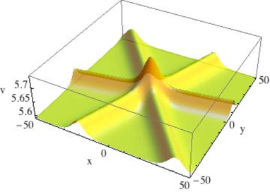
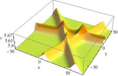
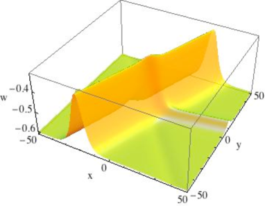
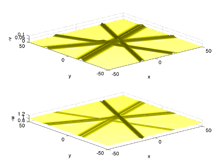
where dots denote certain explicit functions of a,b,c๐‘Ž๐‘๐‘a,b,c which are bounded along with their first order derivatives. Thus, for sufficiently small ฯตitalic-ฯต\epsilon the change of variables a,b,cโ†’x,y,tformulae-sequenceโ†’๐‘Ž๐‘๐‘๐‘ฅ๐‘ฆ๐‘กa,b,c\to x,y,t is nonsingular and well-defined globally, so that the corresponding v๐‘ฃv and w๐‘คw will also be nonsingular. Expressing c๐‘c in the form c=โˆ’tโˆ’aโˆ’b๐‘๐‘ก๐‘Ž๐‘c=-t-a-b and substituting into the formulas (27) for v๐‘ฃv, w๐‘คw, and the first two equations (26), one obtains v,w,x,y๐‘ฃ๐‘ค๐‘ฅ๐‘ฆv,w,x,y as functions of a๐‘Ža and b๐‘b. Thus, one can construct parametric plots of vโ€‹(x,y,t)๐‘ฃ๐‘ฅ๐‘ฆ๐‘กv(x,y,t) and wโ€‹(x,y,t)๐‘ค๐‘ฅ๐‘ฆ๐‘กw(x,y,t). Figs. 7 and 8 show snapshots of v๐‘ฃv and w๐‘คw at t=0๐‘ก0t=0 and t=6๐‘ก6t=6 for the parameter values ฮฑ=1โˆ’(1+tan(ฯ•+ฯ€/3)(1+tan(ฯ•โˆ’ฯ€/3))1+tanโกฯ•,ฮฒ=1โˆ’(1+tanโกฯ•)โ€‹(1+tanโก(ฯ•โˆ’ฯ€/3))1+tanโก(ฯ•+ฯ€/3),ฮณ=1โˆ’(1+tanโกฯ•)โ€‹(1+tanโก(ฯ•+ฯ€/3))1+tanโก(ฯ•โˆ’ฯ€/3)\alpha=1-\sqrt{\frac{(1+\tan(\phi+\pi/3)(1+\tan(\phi-\pi/3))}{1+\tan\phi}},\ \beta=1-\sqrt{\frac{(1+\tan\phi)(1+\tan(\phi-\pi/3))}{1+\tan(\phi+\pi/3)}},\ \gamma=1-\sqrt{\frac{(1+\tan\phi)(1+\tan(\phi+\pi/3))}{1+\tan(\phi-\pi/3)}}, where ฯ•=ฯ€/9italic-ฯ•๐œ‹9\phi=\pi/9, and ฮผ=1,ฯต=0.05formulae-sequence๐œ‡1italic-ฯต0.05\mu=1,\ \epsilon=0.05. At t=0๐‘ก0t=0 initial profiles represent three solitons having a triple collision at the origin (parameters are chosen in such a way that solitons meet at equal angles ฯ€/3๐œ‹3\pi/3). The triple collision then disintegrates into pairwise interactions, shown at t=6๐‘ก6t=6.

Refer to caption
Refer to caption
Figure 7: Solution (27), (28) to the system (5) for v๐‘ฃv at t=0๐‘ก0t=0 and t=6๐‘ก6t=6.
Refer to caption
Refer to caption
Figure 8: Solution (27), (28) to the system (5) for w๐‘คw at t=0๐‘ก0t=0 and t=6๐‘ก6t=6.

Unfortunately, for N>3๐‘3N>3 one cannot reduce Eqs. (21) to parametric formulas, and has to solve them numerically.

3.3.3 Plots of N๐‘N-wave interactions

To obtain a more convenient form for explicit integration, we rewrite Eqs. (21) as

โˆซF1Nโˆ’1โ€‹(p1)โ€‹๐‘‘p1+โ‹ฏ+โˆซFNNโˆ’1โ€‹(pN)โ€‹๐‘‘pN=x,โˆซF1Nโˆ’2โ€‹(p1)โ€‹๐‘‘p1+โ‹ฏ+โˆซFNNโˆ’2โ€‹(pN)โ€‹๐‘‘pN=โˆ’y,โˆซF1kโ€‹(p1)โ€‹๐‘‘p1+โ‹ฏ+โˆซFNkโ€‹(pN)โ€‹๐‘‘pN=0,k=1,2,โ€ฆ,Nโˆ’3,p1+โ€ฆ+pN=(โˆ’1)Nโ€‹(yโˆ’t).superscriptsubscript๐น1๐‘1subscript๐‘1differential-dsubscript๐‘1โ‹ฏsuperscriptsubscript๐น๐‘๐‘1subscript๐‘๐‘differential-dsubscript๐‘๐‘๐‘ฅmissing-subexpressionsuperscriptsubscript๐น1๐‘2subscript๐‘1differential-dsubscript๐‘1โ‹ฏsuperscriptsubscript๐น๐‘๐‘2subscript๐‘๐‘differential-dsubscript๐‘๐‘๐‘ฆmissing-subexpressionformulae-sequencesuperscriptsubscript๐น1๐‘˜subscript๐‘1differential-dsubscript๐‘1โ‹ฏsuperscriptsubscript๐น๐‘๐‘˜subscript๐‘๐‘differential-dsubscript๐‘๐‘0๐‘˜12โ€ฆ๐‘3missing-subexpressionsubscript๐‘1โ€ฆsubscript๐‘๐‘superscript1๐‘๐‘ฆ๐‘ก\begin{array}[]{c}\int F_{1}^{N-1}(p_{1})dp_{1}+\dots+\int F_{N}^{N-1}(p_{N})dp_{N}=x,\\ \\ \int F_{1}^{N-2}(p_{1})dp_{1}+\dots+\int F_{N}^{N-2}(p_{N})dp_{N}=-y,\\ \\ \int F_{1}^{k}(p_{1})dp_{1}+\dots+\int F_{N}^{k}(p_{N})dp_{N}=0,~{}~{}~{}k=1,2,...,N-3,\\ \\ p_{1}+...+p_{N}=(-1)^{N}(y-t).\end{array} (29)

here Fiโ€‹(pi)subscript๐น๐‘–subscript๐‘๐‘–F_{i}(p_{i}) are arbitrary functions, and all integrals are understood as indefinite. The corresponding solution of (5) is given by the formulae

v=โˆ’โˆ‘Fiโ€‹(pi),w=โˆFiโ€‹(pi).formulae-sequence๐‘ฃsubscript๐น๐‘–subscript๐‘๐‘–๐‘คproductsubscript๐น๐‘–subscript๐‘๐‘–v=-\sum F_{i}(p_{i}),~{}~{}~{}w=\prod F_{i}(p_{i}).

Formulae (21) and (29) are identified upon setting Ri=Fi(pi),โˆซRidโ€‹ฮพfiโ€‹(ฮพ)=piR^{i}=F_{i}(p_{i}),\ \stackrel{{\scriptstyle R^{i}}}{{\int}}\frac{d\xi}{f_{i}(\xi)}=p_{i}. Equations (29) can be used to construct nonlinear interactions of N๐‘N soliton-like profiles by taking, e.g., Fiโ€‹(pi)=ฮฑi+ฯตcosh2โกฮผiโ€‹pisubscript๐น๐‘–subscript๐‘๐‘–subscript๐›ผ๐‘–italic-ฯตsuperscript2subscript๐œ‡๐‘–subscript๐‘๐‘–F_{i}(p_{i})=\alpha_{i}+\frac{\epsilon}{\cosh^{2}\mu_{i}p_{i}}, where ฯตitalic-ฯต\epsilon is sufficiently small and the constants ฮฑisubscript๐›ผ๐‘–\alpha_{i} are chosen in such a way that equations (29) are uniquely solvable for piโ€‹(x,y,t)subscript๐‘๐‘–๐‘ฅ๐‘ฆ๐‘กp_{i}(x,y,t).

This approach can in principle be used to build hump-like initial data by letting N๐‘N tend to infinity, thus providing in a loose sense a non-linear generalization of Fourier analysis for the studied PDE. We illustrate this concept below by studying examples for finite N๐‘N numerically. The idea is to construct for t=0๐‘ก0t=0 a central hump from N๐‘N elementary solutions of the form of the KdV soliton.

The angles between these elementary solutions are chosen to be equal. From the second relation in (20) it can be seen that a condition on these angles is equivalent to a condition on the ฮฑisubscript๐›ผ๐‘–\alpha_{i},

โˆ‘j=1Nฮฑjโˆ’ฮฑiโˆ’1ฮฑiโ€‹โˆj=1Nฮฑj=tanโกฯˆi,i=1,โ€ฆ,N.formulae-sequencesuperscriptsubscript๐‘—1๐‘subscript๐›ผ๐‘—subscript๐›ผ๐‘–1subscript๐›ผ๐‘–superscriptsubscriptproduct๐‘—1๐‘subscript๐›ผ๐‘—subscript๐œ“๐‘–๐‘–1โ€ฆ๐‘\sum_{j=1}^{N}\alpha_{j}-\alpha_{i}-\frac{1}{\alpha_{i}}\prod_{j=1}^{N}\alpha_{j}=\tan\psi_{i},\quad i=1,\ldots,N. (30)

To ensure that wโ€‹(x,y,0)<0๐‘ค๐‘ฅ๐‘ฆ00w(x,y,0)<0 we choose Fi=ฮฑi+ฯตcosh2โกฮผiโ€‹pisubscript๐น๐‘–subscript๐›ผ๐‘–italic-ฯตsuperscript2subscript๐œ‡๐‘–subscript๐‘๐‘–F_{i}=\alpha_{i}+\frac{\epsilon}{\cosh^{2}\mu_{i}p_{i}} for i=1,โ€ฆ,Nโˆ’2๐‘–1โ€ฆ๐‘2i=1,\ldots,N-2 and Fi=ฮฑisubscript๐น๐‘–subscript๐›ผ๐‘–F_{i}=\alpha_{i} for i=Nโˆ’1,N๐‘–๐‘1๐‘i=N-1,N. In addition we fix โˆ‘j=1Nฮฑj=0superscriptsubscript๐‘—1๐‘subscript๐›ผ๐‘—0\sum_{j=1}^{N}\alpha_{j}=0 and โˆj=1Nฮฑj=โˆ’1superscriptsubscriptproduct๐‘—1๐‘subscript๐›ผ๐‘—1\prod_{j=1}^{N}\alpha_{j}=-1, thus assuring that we are studying solutions on the zero background for v๐‘ฃv and on the โˆ’11-1 background for w๐‘คw. The first Nโˆ’2๐‘2N-2 ฮฑisubscript๐›ผ๐‘–\alpha_{i} then follow from (30) via the quadratic relations,

1/ฮฑiโˆ’ฮฑi=tanโกฯˆi,i=1,โ€ฆ,Nโˆ’2.formulae-sequence1subscript๐›ผ๐‘–subscript๐›ผ๐‘–subscript๐œ“๐‘–๐‘–1โ€ฆ๐‘21/\alpha_{i}-\alpha_{i}=\tan\psi_{i},\quad i=1,\ldots,N-2.

The remaining two ฮฑisubscript๐›ผ๐‘–\alpha_{i} are a consequence of the condition of vanishing sum of the ฮฑisubscript๐›ผ๐‘–\alpha_{i} and product equal to โˆ’11-1,

ฮฑNโˆ’1,N=12โ€‹(โˆ‘j=1Nโˆ’2ฮฑjยฑ(โˆ‘j=1Nโˆ’2ฮฑj)2โˆ’4โˆj=1Nโˆ’2ฮฑj).subscript๐›ผ๐‘1๐‘12plus-or-minussuperscriptsubscript๐‘—1๐‘2subscript๐›ผ๐‘—superscriptsuperscriptsubscript๐‘—1๐‘2subscript๐›ผ๐‘—24superscriptsubscriptproduct๐‘—1๐‘2subscript๐›ผ๐‘—\alpha_{N-1,N}=\frac{1}{2}\left(\sum_{j=1}^{N-2}\alpha_{j}\pm\sqrt{\left(\sum_{j=1}^{N-2}\alpha_{j}\right)^{2}-\frac{4}{\prod_{j=1}^{N-2}\alpha_{j}}}\right).

The ฯˆisubscript๐œ“๐‘–\psi_{i} are chosen in a way to generate equal angles between the elementary solutions in the (x,y)โˆ’limit-from๐‘ฅ๐‘ฆ(x,y)-plane for t=0๐‘ก0t=0. For numerical reasons one has to avoid ฯˆ=ฯ€/2๐œ“๐œ‹2\psi=\pi/2 since the tangent diverges there. To obtain finite ฯˆisubscript๐œ“๐‘–\psi_{i} also for even N๐‘N, we shift them by a common factor, thus

ฯˆn={nโ€‹ฯ€Nโˆ’2Nโ€‹ย odd,nโ€‹ฯ€Nโˆ’2+ฯ€2โ€‹(Nโˆ’2)Nโ€‹ย even.subscript๐œ“๐‘›cases๐‘›๐œ‹๐‘2๐‘ย odd,๐‘›๐œ‹๐‘2๐œ‹2๐‘2๐‘ย even.\psi_{n}=\begin{cases}\frac{n\pi}{N-2}&N\mbox{ odd,}\\ \frac{n\pi}{N-2}+\frac{\pi}{2(N-2)}&N\mbox{ even.}\end{cases}

With this choice we assure that the values for tanโกฯˆ๐œ“\tan\psi are as small as possible. This is numerically important since the ฮฑisubscript๐›ผ๐‘–\alpha_{i} appear in an Nร—N๐‘๐‘N\times N Vandermonde determinant, i.e., there will be N๐‘Nth powers of each ฮฑisubscript๐›ผ๐‘–\alpha_{i}. For the same reason we also have to choose the signs carefully to avoid too large or too small values of ฮฑNโˆ’1,Nsubscript๐›ผ๐‘1๐‘\alpha_{N-1,N}. With the above choice of the ฯˆisubscript๐œ“๐‘–\psi_{i}, i=1,โ€ฆ,Nโˆ’2๐‘–1โ€ฆ๐‘2i=1,\ldots,N-2, we have assured that with some ฮฑjsubscript๐›ผ๐‘—\alpha_{j} a solution to one of the equations (30), also โˆ’ฮฑjsubscript๐›ผ๐‘—-\alpha_{j} and ยฑฮฑjplus-or-minussubscript๐›ผ๐‘—\pm\alpha_{j} are solutions to these equations (either for ฯˆjsubscript๐œ“๐‘—\psi_{j} or for ฯ€โˆ’ฯˆj๐œ‹subscript๐œ“๐‘—\pi-\psi_{j}). We fix the signs in a way to obtain a minimal โˆ‘i=1Nโˆ’2ฮฑisuperscriptsubscript๐‘–1๐‘2subscript๐›ผ๐‘–\sum_{i=1}^{N-2}\alpha_{i} and a negative โˆi=1Nโˆ’2ฮฑisuperscriptsubscriptproduct๐‘–1๐‘2subscript๐›ผ๐‘–\prod_{i=1}^{N-2}\alpha_{i}. This is done by alternating the signs in the ฮฑisubscript๐›ผ๐‘–\alpha_{i}, i=1,โ€ฆ,Nmโ€‹aโ€‹x๐‘–1โ€ฆsubscript๐‘๐‘š๐‘Ž๐‘ฅi=1,\ldots,N_{max} (Nmโ€‹aโ€‹x=N/2โˆ’1subscript๐‘๐‘š๐‘Ž๐‘ฅ๐‘21N_{max}=N/2-1 for N๐‘N even and Nmโ€‹aโ€‹x=(Nโˆ’1)/2subscript๐‘๐‘š๐‘Ž๐‘ฅ๐‘12N_{max}=(N-1)/2 for N๐‘N odd). The remaining signs are chosen in a way that the ฮฑjsubscript๐›ผ๐‘—\alpha_{j} corresponding to ฯ€โˆ’ฯˆi๐œ‹subscript๐œ“๐‘–\pi-\psi_{i} is equal to 1/ฮฑi1subscript๐›ผ๐‘–1/\alpha_{i}. Thus we assure that ฮฑNโˆ’1subscript๐›ผ๐‘1\alpha_{N-1} and ฮฑNsubscript๐›ผ๐‘\alpha_{N} are real and that 1/|ฮฑNmโ€‹aโ€‹x|โ‰ค|ฮฑi|โ‰ค|ฮฑNmโ€‹aโ€‹x|1subscript๐›ผsubscript๐‘๐‘š๐‘Ž๐‘ฅsubscript๐›ผ๐‘–subscript๐›ผsubscript๐‘๐‘š๐‘Ž๐‘ฅ1/|\alpha_{N_{max}}|\leq|\alpha_{i}|\leq|\alpha_{N_{max}}|. We give the values of the ฮฑisubscript๐›ผ๐‘–\alpha_{i} for two examples below. Since ฮฑNmโ€‹aโ€‹xโˆผ2โ€‹(Nโˆ’2)/ฯ€similar-tosubscript๐›ผsubscript๐‘๐‘š๐‘Ž๐‘ฅ2๐‘2๐œ‹\alpha_{N_{max}}\sim 2(N-2)/\pi, we can in double precision reach values of N=14๐‘14N=14 in which case the conditioning of the Vandermonde matrix of the ฮฑisubscript๐›ผ๐‘–\alpha_{i} is of the order of 10โˆ’14superscript101410^{-14} (the absolute value of the ratio of the smallest to the largest eigenvalue of the matrix). To treat higher values of N๐‘N more than double precision is needed which is, however, beyond the scope of this paper.

The goal of this subsection is to construct for t=0๐‘ก0t=0 a single hump for v๐‘ฃv with value c=cโ€‹oโ€‹nโ€‹sโ€‹t๐‘๐‘๐‘œ๐‘›๐‘ ๐‘กc=const at x=y=0๐‘ฅ๐‘ฆ0x=y=0. To this end we choose ฯต=c/(Nโˆ’2)italic-ฯต๐‘๐‘2\epsilon=c/(N-2) since Nโˆ’2๐‘2N-2 elementary solutions will overlap at the origin of the (x,y)๐‘ฅ๐‘ฆ(x,y) plane with the above choices. Thus we take ฯต=c/(Nโˆ’2)italic-ฯต๐‘๐‘2\epsilon=c/(N-2) and take c=0.1๐‘0.1c=0.1. The constant c๐‘c has to be chosen in a way that w๐‘คw remains negative which seems to be the case in the numerical experiments discussed below if c<1๐‘1c<1. A smaller value of c๐‘c leads to a more rapid convergence of the iteration to be described below.

For the given form of the Fisubscript๐น๐‘–F_{i}, i=1,โ€ฆ,N๐‘–1โ€ฆ๐‘i=1,...,N, we have (nโ‰ฅ1๐‘›1n\geq 1)

โˆซFinโ€‹(pi)โ€‹๐‘‘pi=ฮฑinโ€‹pi+โˆ‘j=1n(nj)โ€‹ฯตjโ€‹ฮฑinโˆ’jโ€‹Ijโ€‹(pi),superscriptsubscript๐น๐‘–๐‘›subscript๐‘๐‘–differential-dsubscript๐‘๐‘–superscriptsubscript๐›ผ๐‘–๐‘›subscript๐‘๐‘–superscriptsubscript๐‘—1๐‘›matrix๐‘›๐‘—superscriptitalic-ฯต๐‘—superscriptsubscript๐›ผ๐‘–๐‘›๐‘—subscript๐ผ๐‘—subscript๐‘๐‘–\int F_{i}^{n}(p_{i})dp_{i}=\alpha_{i}^{n}p_{i}+\sum_{j=1}^{n}\begin{pmatrix}n\\ j\end{pmatrix}\epsilon^{j}\alpha_{i}^{n-j}I_{j}(p_{i}),

where Inโ€‹(p)=โˆซp๐‘‘pโ€ฒ/cosh2โ€‹nโกpโ€ฒsubscript๐ผ๐‘›๐‘superscript๐‘differential-dsuperscript๐‘โ€ฒsuperscript2๐‘›superscript๐‘โ€ฒI_{n}(p)=\int^{p}dp^{\prime}/\cosh^{2n}p^{\prime}. Equations (29) thus take the form (k=1,2,โ€ฆ,Nโˆ’3๐‘˜12โ€ฆ๐‘3k=1,2,\ldots,N-3)

โˆ‘i=1Nโˆ’2{ฮฑiNโˆ’1โ€‹pi+โˆ‘j=1Nโˆ’1(Nโˆ’1j)โ€‹ฯตjโ€‹ฮฑiNโˆ’1โˆ’jโ€‹Ijโ€‹(pi)}+ฮฑNโˆ’1Nโˆ’1โ€‹pNโˆ’1+ฮฑNNโˆ’1โ€‹pNsuperscriptsubscript๐‘–1๐‘2superscriptsubscript๐›ผ๐‘–๐‘1subscript๐‘๐‘–superscriptsubscript๐‘—1๐‘1matrix๐‘1๐‘—superscriptitalic-ฯต๐‘—superscriptsubscript๐›ผ๐‘–๐‘1๐‘—subscript๐ผ๐‘—subscript๐‘๐‘–subscriptsuperscript๐›ผ๐‘1๐‘1subscript๐‘๐‘1superscriptsubscript๐›ผ๐‘๐‘1subscript๐‘๐‘\displaystyle\sum_{i=1}^{N-2}\left\{\alpha_{i}^{N-1}p_{i}+\sum_{j=1}^{N-1}\begin{pmatrix}N-1\\ j\end{pmatrix}\epsilon^{j}\alpha_{i}^{N-1-j}I_{j}(p_{i})\right\}+\alpha^{N-1}_{N-1}p_{N-1}+\alpha_{N}^{N-1}p_{N} =x,absent๐‘ฅ\displaystyle=x,
โˆ‘i=1Nโˆ’2{ฮฑiNโˆ’2โ€‹pi+โˆ‘j=1Nโˆ’2(Nโˆ’2j)โ€‹ฯตjโ€‹ฮฑiNโˆ’2โˆ’jโ€‹Ijโ€‹(pi)}+ฮฑNโˆ’1Nโˆ’2โ€‹pNโˆ’1+ฮฑNNโˆ’2โ€‹pNsuperscriptsubscript๐‘–1๐‘2superscriptsubscript๐›ผ๐‘–๐‘2subscript๐‘๐‘–superscriptsubscript๐‘—1๐‘2matrix๐‘2๐‘—superscriptitalic-ฯต๐‘—superscriptsubscript๐›ผ๐‘–๐‘2๐‘—subscript๐ผ๐‘—subscript๐‘๐‘–subscriptsuperscript๐›ผ๐‘2๐‘1subscript๐‘๐‘1superscriptsubscript๐›ผ๐‘๐‘2subscript๐‘๐‘\displaystyle\sum_{i=1}^{N-2}\left\{\alpha_{i}^{N-2}p_{i}+\sum_{j=1}^{N-2}\begin{pmatrix}N-2\\ j\end{pmatrix}\epsilon^{j}\alpha_{i}^{N-2-j}I_{j}(p_{i})\right\}+\alpha^{N-2}_{N-1}p_{N-1}+\alpha_{N}^{N-2}p_{N} =โˆ’yabsent๐‘ฆ\displaystyle=-y
โˆ‘i=1Nโˆ’2{ฮฑikโ€‹pi+โˆ‘j=1k(kj)โ€‹ฯตjโ€‹ฮฑikโˆ’jโ€‹Ijโ€‹(pi)}+ฮฑNโˆ’1kโ€‹pNโˆ’1+ฮฑNkโ€‹pNsuperscriptsubscript๐‘–1๐‘2superscriptsubscript๐›ผ๐‘–๐‘˜subscript๐‘๐‘–superscriptsubscript๐‘—1๐‘˜matrix๐‘˜๐‘—superscriptitalic-ฯต๐‘—superscriptsubscript๐›ผ๐‘–๐‘˜๐‘—subscript๐ผ๐‘—subscript๐‘๐‘–subscriptsuperscript๐›ผ๐‘˜๐‘1subscript๐‘๐‘1superscriptsubscript๐›ผ๐‘๐‘˜subscript๐‘๐‘\displaystyle\sum_{i=1}^{N-2}\left\{\alpha_{i}^{k}p_{i}+\sum_{j=1}^{k}\begin{pmatrix}k\\ j\end{pmatrix}\epsilon^{j}\alpha_{i}^{k-j}I_{j}(p_{i})\right\}+\alpha^{k}_{N-1}p_{N-1}+\alpha_{N}^{k}p_{N} =0,absent0\displaystyle=0,
p1+โ€ฆ+pNsubscript๐‘1โ€ฆsubscript๐‘๐‘\displaystyle p_{1}+\ldots+p_{N} =(โˆ’1)Nโ€‹(yโˆ’t),absentsuperscript1๐‘๐‘ฆ๐‘ก\displaystyle=(-1)^{N}(y-t),

This system can be solved iteratively. Let V๐‘‰V be the Vandermonde determinant of the ฮฑisubscript๐›ผ๐‘–\alpha_{i}. Then we solve iteratively for the vector pโ†’โ†’๐‘\vec{p}, where pโ†’n+1subscriptโ†’๐‘๐‘›1\vec{p}_{n+1} follows from the n๐‘›nth iterate via

Vโ€‹pโ†’n+1=Jโ†’โ€‹(pโ†’n),๐‘‰subscriptโ†’๐‘๐‘›1โ†’๐ฝsubscriptโ†’๐‘๐‘›V\vec{p}_{n+1}=\vec{J}(\vec{p}_{n}),

with

J1โ€‹(pโ†’n)=โˆ’โˆ‘i=1Nโˆ’2โˆ‘j=1Nโˆ’1(Nโˆ’1j)โ€‹ฯตjโ€‹ฮฑiNโˆ’1โˆ’jโ€‹Ijโ€‹(pi)+x,subscript๐ฝ1subscriptโ†’๐‘๐‘›superscriptsubscript๐‘–1๐‘2superscriptsubscript๐‘—1๐‘1matrix๐‘1๐‘—superscriptitalic-ฯต๐‘—subscriptsuperscript๐›ผ๐‘1๐‘—๐‘–subscript๐ผ๐‘—subscript๐‘๐‘–๐‘ฅJ_{1}(\vec{p}_{n})=-\sum_{i=1}^{N-2}\sum_{j=1}^{N-1}\begin{pmatrix}N-1\\ j\end{pmatrix}\epsilon^{j}\alpha^{N-1-j}_{i}I_{j}(p_{i})+x,

etc, and

Jโ†’โ€‹(pโ†’0)=(x,โˆ’y,0,โ€ฆ,0,(โˆ’1)Nโ€‹(yโˆ’t)).โ†’๐ฝsubscriptโ†’๐‘0๐‘ฅ๐‘ฆ0โ€ฆ0superscript1๐‘๐‘ฆ๐‘ก\vec{J}(\vec{p}_{0})=(x,-y,0,\ldots,0,(-1)^{N}(y-t)).

The iteration is stopped once |pโ†’n+1โˆ’pโ†’n|<ฮดsubscriptโ†’๐‘๐‘›1subscriptโ†’๐‘๐‘›๐›ฟ|\vec{p}_{n+1}-\vec{p}_{n}|<\delta (we use ฮด=10โˆ’6๐›ฟsuperscript106\delta=10^{-6}). For a value of cโ‰ช1much-less-than๐‘1c\ll 1, this iteration converges rapidly (typically less than 4 iterations). If cโˆผ1similar-to๐‘1c\sim 1 the iteration converges only slowly or not at all.

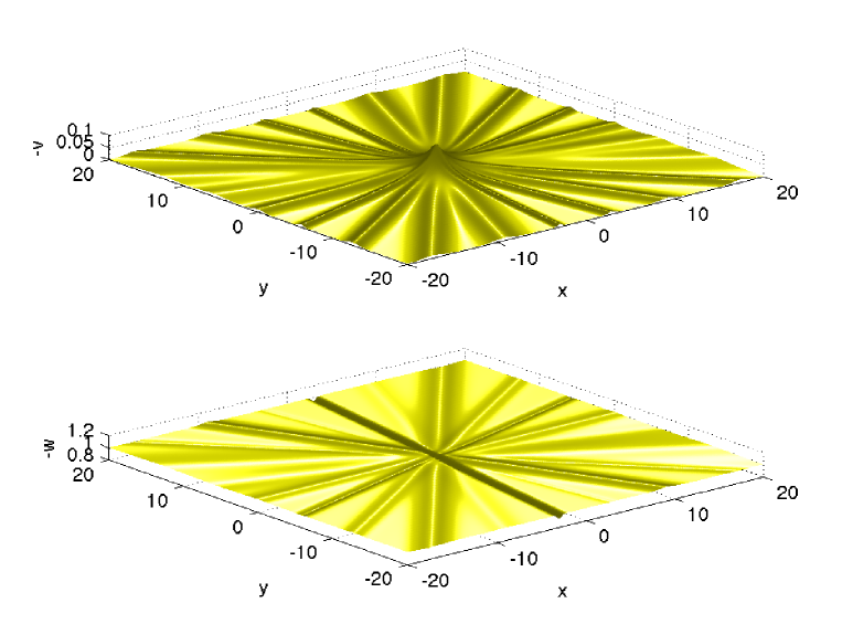
The results of the above procedure for N=6๐‘6N=6 (four elementary solutions) for t=0๐‘ก0t=0 can be seen in Fig.ย 9. Since this approach is concerned with hump-like structures in v๐‘ฃv, the outcome for w๐‘คw is not obvious, but can be seen in the lower part.
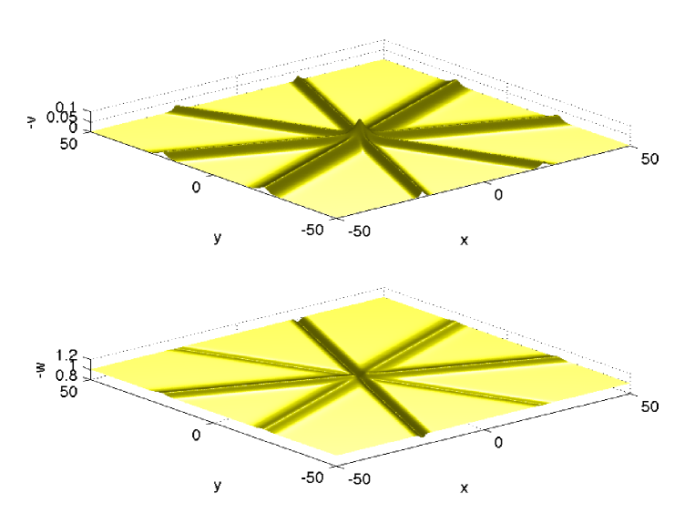
Refer to caption
Figure 9: Solutions v๐‘ฃv and w๐‘คw to the system (29) for N=6๐‘6N=6 at t=0๐‘ก0t=0 and ฮผโ†’=(1,100,1,1)โ†’๐œ‡110011\vec{\mu}=(1,100,1,1). The values of ฮผโ†’โ†’๐œ‡\vec{\mu} have been chosen in a way that the lateral extension of the elementary waves is of a similar order. This implies ฮฑโ†’โ‰ˆ(0.81,โˆ’2.77,โˆ’0.36,1.23,โˆ’0.59,1.69)โ†’๐›ผ0.812.770.361.230.591.69\vec{\alpha}\approx(0.81,-2.77,-0.36,1.23,-0.59,1.69).

The central hump for v๐‘ฃv at the origin of the (x,y)๐‘ฅ๐‘ฆ(x,y)-plane disintegrates with time as can be seen in Fig.ย 10.

Refer to caption
Figure 10: Solutions v๐‘ฃv and w๐‘คw to the system (29) for N=6๐‘6N=6 at t=6๐‘ก6t=6 and ฮผโ†’=(1,100,1,1)โ†’๐œ‡110011\vec{\mu}=(1,100,1,1).

Since we fixed the maximum of the absolute value of v๐‘ฃv at the center to be of the order of c๐‘c, the relative maximum of the modulus of the elementary waves tends with large N๐‘N to 0. This is illustrated in Fig.ย 11 for N=13๐‘13N=13.

Refer to caption
Figure 11: Solutions v๐‘ฃv and w๐‘คw to the system (29) for N=13๐‘13N=13 at t=0๐‘ก0t=0 and ฮผโ†’=(100,100,10,104,10,1010,1,105,10,103,100)โ†’๐œ‡10010010superscript10410superscript10101superscript10510superscript103100\vec{\mu}=(100,100,10,10^{4},10,10^{10},1,10^{5},10,10^{3},100). The values of ฮผโ†’โ†’๐œ‡\vec{\mu} have been chosen in a way that the lateral extension of the elementary waves is of a similar order. This implies ฮฑโ†’โ‰ˆ(1.00,โˆ’1.16,0.73,โˆ’1.73,0.39,โˆ’7.10,โˆ’0.14,2.58,โˆ’0.58,1.37,โˆ’0.86,โˆ’0.18,5.68)โ†’๐›ผ1.001.160.731.730.397.100.142.580.581.370.860.185.68\vec{\alpha}\approx(1.00,-1.16,0.73,-1.73,0.39,-7.10,-0.14,2.58,-0.58,1.37,-0.86,-0.18,5.68).

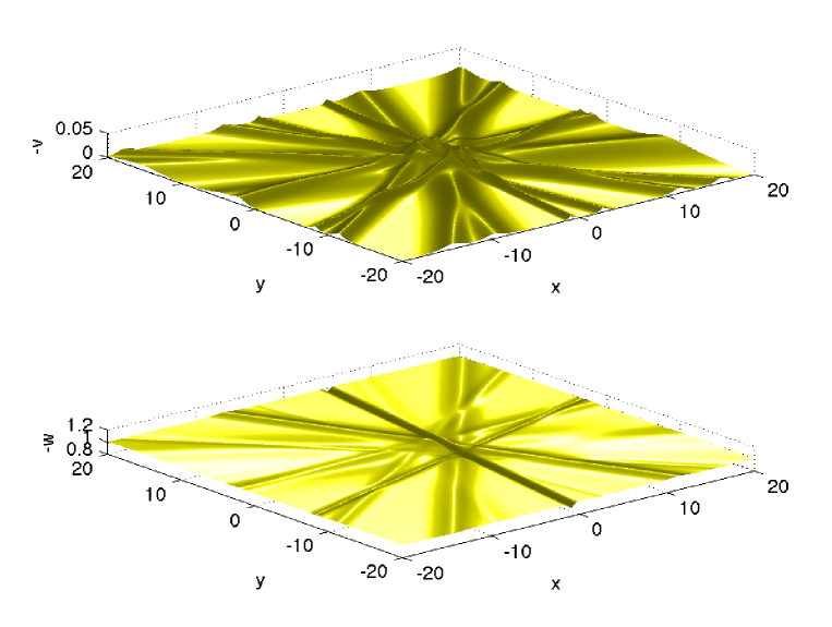
The central hump for v๐‘ฃv at the origin of the (x,y)๐‘ฅ๐‘ฆ(x,y)-plane disintegrates with time as can be seen in Fig.ย 12. Compare this figure with the time evolution of hump-like initial data for v๐‘ฃv studied numerically in the next subsection.
Refer to caption
Figure 12: Solutions v๐‘ฃv and w๐‘คw to the system (29) for N=13๐‘13N=13 at t=2๐‘ก2t=2 and ฮผโ†’=(100,100,10,104,10,1010,1,105,10,103,100)โ†’๐œ‡10010010superscript10410superscript10101superscript10510superscript103100\vec{\mu}=(100,100,10,10^{4},10,10^{10},1,10^{5},10,10^{3},100).

3.4 Cauchy problems and numerical evaluations

We will use the Friedrichs-symmetrized form (10), which is well-posed for w<0๐‘ค0w<0, for numerical simulations of system (5). The task is to investigate the conjecture that solutions to the system (5) for generic initial data do not develop a point of gradient catastrophe in finite time.

To this end we consider initial data in the Schwartzian class of rapidly decreasing functions. Such functions can be treated for numerical purposes as effectively periodic if the period is chosen large enough that the studied functions decrease below the machine precision (which is of the order 10โˆ’16superscript101610^{-16} for double precision computations in MATLAB [29]) at the ends of the intervals. The Gibbs phenomenon in such a case is of the order of the rounding error and thus negligible. This setting allows the use of Fourier spectral methods which are known for their excellent approximation properties for smooth functions. Thus we will approximate the spatial dependence of the functions v๐‘ฃv and w๐‘คw via discrete Fourier series. We find that the solutions to the system (5) stay in the Schwartzian class in contrast, e.g., to solutions to the dispersionless Kadomtsev-Petviashvili (dKP) equation, see [21] for a numerical study.

The time dependence is treated via a standard fourth order Runge-Kutta scheme. The quality of the numerics is controlled via the conserved quantity

I:=โˆซโˆ’โˆžโˆžโˆซโˆ’โˆžโˆž(v2โˆ’(wโˆ’wโˆž))โ€‹๐‘‘xโ€‹๐‘‘yassign๐ผsuperscriptsubscriptsuperscriptsubscriptsuperscript๐‘ฃ2๐‘คsubscript๐‘คdifferential-d๐‘ฅdifferential-d๐‘ฆI:=\int_{-\infty}^{\infty}\int_{-\infty}^{\infty}(v^{2}-(w-w_{\infty}))dxdy

of system (5), where wโˆž=limx,yโ†’โˆžwโ€‹(x,y,t)subscript๐‘คsubscriptโ†’๐‘ฅ๐‘ฆ๐‘ค๐‘ฅ๐‘ฆ๐‘กw_{\infty}=\lim_{x,y\to\infty}w(x,y,t). Since the conservation of this quantity is not implemented in the code, it will not be exactly observed in actual numerical experiments due to unavoidable numerical errors. Thus the numerical conservation of I๐ผI can serve as an indicator for the achieved accuracy. In our experiments the error in the relative conservation of this quantity was below 10โˆ’6superscript10610^{-6}. It is known (see for instance [22]) that integral quantities overestimate the accuracy in a Lโˆžsubscript๐ฟL_{\infty} sense of numerical solutions to a partial differential equations by one to two orders of magnitude. Thus the results presented below are accurate to at least 10โˆ’4superscript10410^{-4} which is well beyond plotting accuracy. Comparing the behavior of the numerical solutions to solutions to the dKP equation in [21] which show blow up, we see in the experiments performed below no indication of an increasing gradient of the solutions. Thus it seems that at least for the class of initial data considered, the numerical solutions will have global existence in time.

As a concrete example we study the initial data vโ€‹(x,y,0)=expโก(โˆ’(x2+y2))๐‘ฃ๐‘ฅ๐‘ฆ0superscript๐‘ฅ2superscript๐‘ฆ2v(x,y,0)=\exp(-(x^{2}+y^{2})) and wโ€‹(x,y,0)=โˆ’1๐‘ค๐‘ฅ๐‘ฆ01w(x,y,0)=-1. It can be seen in Fig.ย 13 that the solution for v๐‘ฃv stays smooth and localized in both spatial directions.
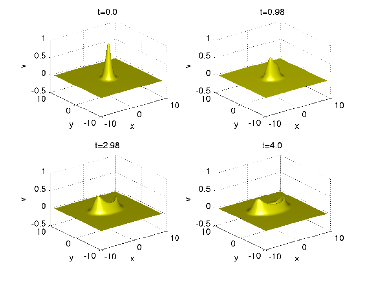
Refer to caption
Figure 13: Solution v๐‘ฃv to the system (5) for the initial data vโ€‹(x,y,0)=expโก(โˆ’(x2+y2))๐‘ฃ๐‘ฅ๐‘ฆ0superscript๐‘ฅ2superscript๐‘ฆ2v(x,y,0)=\exp(-(x^{2}+y^{2})) and wโ€‹(x,y,0)=โˆ’1๐‘ค๐‘ฅ๐‘ฆ01w(x,y,0)=-1 for several values of t๐‘กt.

A similar behavior can be observed for the solution w๐‘คw in Fig.ย 14. This solution starts with w=โˆ’1๐‘ค1w=-1 and develops peaks above and below this initial surface. It can be seen that both functions v๐‘ฃv and w๐‘คw approach an elliptic shape which could indicate the existence of an elliptic localized solution which acts as an attractor for a wide class of initial data.
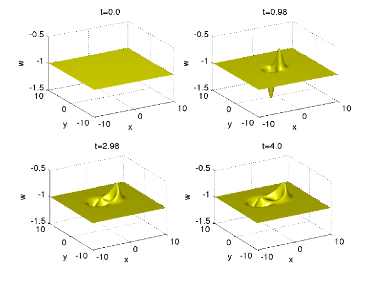
Refer to caption
Figure 14: Solution w๐‘คw to the system (5) for the initial data vโ€‹(x,y,0)=expโก(โˆ’(x2+y2))๐‘ฃ๐‘ฅ๐‘ฆ0superscript๐‘ฅ2superscript๐‘ฆ2v(x,y,0)=\exp(-(x^{2}+y^{2})) and wโ€‹(x,y,0)=โˆ’1๐‘ค๐‘ฅ๐‘ฆ01w(x,y,0)=-1 for several values of t๐‘กt.

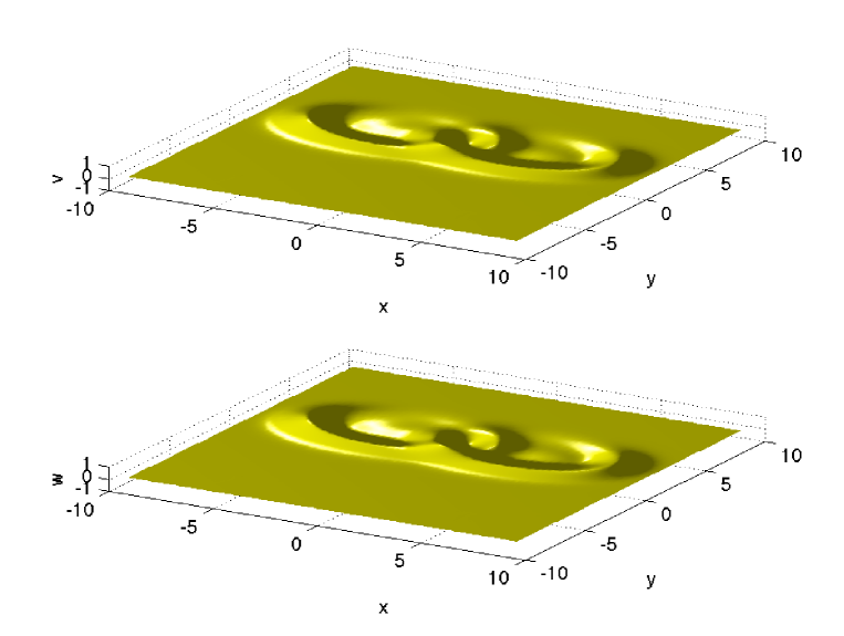
The elliptic shape seems to be also present if one starts with several humps. In Fig.ย 15 we consider initial data of the form vโ€‹(x,y,0)=expโก(โˆ’((xโˆ’3)2+y2))+expโก(โˆ’((x+3)2+y2))๐‘ฃ๐‘ฅ๐‘ฆ0superscript๐‘ฅ32superscript๐‘ฆ2superscript๐‘ฅ32superscript๐‘ฆ2v(x,y,0)=\exp(-((x-3)^{2}+y^{2}))+\exp(-((x+3)^{2}+y^{2})) and wโ€‹(x,y,0)=โˆ’1๐‘ค๐‘ฅ๐‘ฆ01w(x,y,0)=-1. As can be seen both humps develop into an ellipse. The behavior for w๐‘คw is as follows: since it starts as identically constant, two humps of opposite sign are forming. Both develop then an elliptic shape as seen in Fig.ย ย 15.

Refer to caption
Figure 15: Solutions v๐‘ฃv and w๐‘คw to the system (5) for the initial data vโ€‹(x,y,0)=expโก(โˆ’((xโˆ’3)2+y2))+expโก(โˆ’((x+3)2+y2))๐‘ฃ๐‘ฅ๐‘ฆ0superscript๐‘ฅ32superscript๐‘ฆ2superscript๐‘ฅ32superscript๐‘ฆ2v(x,y,0)=\exp(-((x-3)^{2}+y^{2}))+\exp(-((x+3)^{2}+y^{2})) and wโ€‹(x,y,0)=โˆ’1๐‘ค๐‘ฅ๐‘ฆ01w(x,y,0)=-1 for t=4๐‘ก4t=4.

4 Proof of Theorem 1

In Sect. 4.1 we summarize the integrability conditions for two-component (2+1)21(2+1)-dimensional quasilinear systems. Their differential consequences are used in Sect. 4.2 to establish Theorem 1.

4.1 Integrability conditions for 222-component systems in 2+1212+1 dimensions

Here we present the integrability conditions for 222-component quasilinear systems of the form (2). Setting ๐ฎ=(v,w)t๐ฎsuperscript๐‘ฃ๐‘ค๐‘ก{\bf u}=(v,w)^{t} and diagonalizing the matrix A๐ดA, which is always possible in the 2ร—2222\times 2 case, one obtains the equations

(vw)t+(a00b)โ€‹(vw)x+(pqrs)โ€‹(vw)y=0.subscript๐‘ฃmissing-subexpression๐‘ค๐‘ก๐‘Ž0missing-subexpressionmissing-subexpression0๐‘subscript๐‘ฃmissing-subexpression๐‘ค๐‘ฅ๐‘๐‘žmissing-subexpressionmissing-subexpression๐‘Ÿ๐‘ subscript๐‘ฃmissing-subexpression๐‘ค๐‘ฆ0\left(\begin{array}[]{c}v\\ \\ w\end{array}\right)_{t}+\left(\begin{array}[]{cc}a&0\\ \\ 0&b\end{array}\right)\left(\begin{array}[]{c}v\\ \\ w\end{array}\right)_{x}+\left(\begin{array}[]{cc}p&q\\ \\ r&s\end{array}\right)\left(\begin{array}[]{c}v\\ \\ w\end{array}\right)_{y}=0. (31)

The integrability conditions constitute a complicated set of second order differential constraints for the coefficients a,b,p,q,r,s๐‘Ž๐‘๐‘๐‘ž๐‘Ÿ๐‘ a,b,p,q,r,s which were derived in [14] based on the method of hydrodynamic reductions.

Equations for a๐‘Ža:

avโ€‹vsubscript๐‘Ž๐‘ฃ๐‘ฃ\displaystyle a_{vv} =\displaystyle= qโ€‹avโ€‹bv+2โ€‹qโ€‹av2+(sโˆ’p)โ€‹avโ€‹awโˆ’rโ€‹aw2(aโˆ’b)โ€‹q+avโ€‹rvr+2โ€‹avโ€‹pwโˆ’awโ€‹pvq,๐‘žsubscript๐‘Ž๐‘ฃsubscript๐‘๐‘ฃ2๐‘žsuperscriptsubscript๐‘Ž๐‘ฃ2๐‘ ๐‘subscript๐‘Ž๐‘ฃsubscript๐‘Ž๐‘ค๐‘Ÿsuperscriptsubscript๐‘Ž๐‘ค2๐‘Ž๐‘๐‘žsubscript๐‘Ž๐‘ฃsubscript๐‘Ÿ๐‘ฃ๐‘Ÿ2subscript๐‘Ž๐‘ฃsubscript๐‘๐‘คsubscript๐‘Ž๐‘คsubscript๐‘๐‘ฃ๐‘ž\displaystyle\frac{\displaystyle{qa_{v}b_{v}+2qa_{v}^{2}+(s-p)a_{v}a_{w}-ra_{w}^{2}}}{\displaystyle{(a-b)q}}+\frac{\displaystyle{a_{v}r_{v}}}{\displaystyle{r}}+\frac{\displaystyle{2a_{v}p_{w}-a_{w}p_{v}}}{\displaystyle{q}},
avโ€‹wsubscript๐‘Ž๐‘ฃ๐‘ค\displaystyle a_{vw} =\displaystyle= avโ€‹aw+bwaโˆ’b+avโ€‹(qwq+rwr),subscript๐‘Ž๐‘ฃsubscript๐‘Ž๐‘คsubscript๐‘๐‘ค๐‘Ž๐‘subscript๐‘Ž๐‘ฃsubscript๐‘ž๐‘ค๐‘žsubscript๐‘Ÿ๐‘ค๐‘Ÿ\displaystyle a_{v}\frac{\displaystyle{a_{w}+b_{w}}}{\displaystyle{a-b}}+a_{v}(\frac{\displaystyle{q_{w}}}{q}+\frac{\displaystyle{r_{w}}}{r}), (32)
awโ€‹wsubscript๐‘Ž๐‘ค๐‘ค\displaystyle a_{ww} =\displaystyle= qโ€‹avโ€‹bv+(sโˆ’p)โ€‹avโ€‹bw+rโ€‹aw2(aโˆ’b)โ€‹r+avโ€‹swr+awโ€‹qwq.๐‘žsubscript๐‘Ž๐‘ฃsubscript๐‘๐‘ฃ๐‘ ๐‘subscript๐‘Ž๐‘ฃsubscript๐‘๐‘ค๐‘Ÿsuperscriptsubscript๐‘Ž๐‘ค2๐‘Ž๐‘๐‘Ÿsubscript๐‘Ž๐‘ฃsubscript๐‘ ๐‘ค๐‘Ÿsubscript๐‘Ž๐‘คsubscript๐‘ž๐‘ค๐‘ž\displaystyle\frac{\displaystyle{qa_{v}b_{v}+(s-p)a_{v}b_{w}+ra_{w}^{2}}}{\displaystyle{(a-b)r}}+\frac{\displaystyle{a_{v}s_{w}}}{r}+\frac{\displaystyle{a_{w}q_{w}}}{q}.

Equations for b๐‘b:

bvโ€‹vsubscript๐‘๐‘ฃ๐‘ฃ\displaystyle b_{vv} =\displaystyle= rโ€‹awโ€‹bw+(pโˆ’s)โ€‹avโ€‹bw+qโ€‹bv2(bโˆ’a)โ€‹q+bwโ€‹pvq+bvโ€‹rvr;๐‘Ÿsubscript๐‘Ž๐‘คsubscript๐‘๐‘ค๐‘๐‘ subscript๐‘Ž๐‘ฃsubscript๐‘๐‘ค๐‘žsuperscriptsubscript๐‘๐‘ฃ2๐‘๐‘Ž๐‘žsubscript๐‘๐‘คsubscript๐‘๐‘ฃ๐‘žsubscript๐‘๐‘ฃsubscript๐‘Ÿ๐‘ฃ๐‘Ÿ\displaystyle\frac{\displaystyle{ra_{w}b_{w}+(p-s)a_{v}b_{w}+qb_{v}^{2}}}{\displaystyle{(b-a)q}}+\frac{\displaystyle{b_{w}p_{v}}}{q}+\frac{\displaystyle{b_{v}r_{v}}}{r};
bvโ€‹wsubscript๐‘๐‘ฃ๐‘ค\displaystyle b_{vw} =\displaystyle= bwโ€‹av+bvbโˆ’a+bwโ€‹(qvq+rvr),subscript๐‘๐‘คsubscript๐‘Ž๐‘ฃsubscript๐‘๐‘ฃ๐‘๐‘Žsubscript๐‘๐‘คsubscript๐‘ž๐‘ฃ๐‘žsubscript๐‘Ÿ๐‘ฃ๐‘Ÿ\displaystyle b_{w}\frac{\displaystyle{a_{v}+b_{v}}}{\displaystyle{b-a}}+b_{w}(\frac{\displaystyle{q_{v}}}{q}+\frac{\displaystyle{r_{v}}}{r}), (33)
bwโ€‹wsubscript๐‘๐‘ค๐‘ค\displaystyle b_{ww} =\displaystyle= rโ€‹awโ€‹bw+2โ€‹rโ€‹bw2+(pโˆ’s)โ€‹bvโ€‹bwโˆ’qโ€‹bv2(bโˆ’a)โ€‹r+bwโ€‹qwq+2โ€‹bwโ€‹svโˆ’bvโ€‹swr.๐‘Ÿsubscript๐‘Ž๐‘คsubscript๐‘๐‘ค2๐‘Ÿsuperscriptsubscript๐‘๐‘ค2๐‘๐‘ subscript๐‘๐‘ฃsubscript๐‘๐‘ค๐‘žsuperscriptsubscript๐‘๐‘ฃ2๐‘๐‘Ž๐‘Ÿsubscript๐‘๐‘คsubscript๐‘ž๐‘ค๐‘ž2subscript๐‘๐‘คsubscript๐‘ ๐‘ฃsubscript๐‘๐‘ฃsubscript๐‘ ๐‘ค๐‘Ÿ\displaystyle\frac{\displaystyle{ra_{w}b_{w}+2rb_{w}^{2}+(p-s)b_{v}b_{w}-qb_{v}^{2}}}{\displaystyle{(b-a)r}}+\frac{\displaystyle{b_{w}q_{w}}}{\displaystyle{q}}+\frac{\displaystyle{2b_{w}s_{v}-b_{v}s_{w}}}{\displaystyle{r}}.

Equations for p๐‘p:

pvโ€‹vsubscript๐‘๐‘ฃ๐‘ฃ\displaystyle p_{vv} =\displaystyle= 2โ€‹rโ€‹(avโ€‹bwโˆ’awโ€‹bv)+(sโˆ’p)โ€‹avโ€‹bv(aโˆ’b)2+rvโ€‹pvr+pvโ€‹pwq+2๐‘Ÿsubscript๐‘Ž๐‘ฃsubscript๐‘๐‘คsubscript๐‘Ž๐‘คsubscript๐‘๐‘ฃ๐‘ ๐‘subscript๐‘Ž๐‘ฃsubscript๐‘๐‘ฃsuperscript๐‘Ž๐‘2subscript๐‘Ÿ๐‘ฃsubscript๐‘๐‘ฃ๐‘Ÿlimit-fromsubscript๐‘๐‘ฃsubscript๐‘๐‘ค๐‘ž\displaystyle 2\frac{r(a_{v}b_{w}-a_{w}b_{v})+(s-p)a_{v}b_{v}}{(a-b)^{2}}+\frac{r_{v}p_{v}}{r}+\frac{p_{v}p_{w}}{q}+
rqโ€‹(2โ€‹qvโ€‹awโˆ’2โ€‹avโ€‹qw+awโ€‹pw)โˆ’bvโ€‹pv+2โ€‹rvโ€‹awโˆ’2โ€‹avโ€‹(sv+pv+rw)+pโˆ’sqโ€‹(2โ€‹pvโ€‹awโˆ’avโ€‹pw)bโˆ’a๐‘Ÿ๐‘ž2subscript๐‘ž๐‘ฃsubscript๐‘Ž๐‘ค2subscript๐‘Ž๐‘ฃsubscript๐‘ž๐‘คsubscript๐‘Ž๐‘คsubscript๐‘๐‘คsubscript๐‘๐‘ฃsubscript๐‘๐‘ฃ2subscript๐‘Ÿ๐‘ฃsubscript๐‘Ž๐‘ค2subscript๐‘Ž๐‘ฃsubscript๐‘ ๐‘ฃsubscript๐‘๐‘ฃsubscript๐‘Ÿ๐‘ค๐‘๐‘ ๐‘ž2subscript๐‘๐‘ฃsubscript๐‘Ž๐‘คsubscript๐‘Ž๐‘ฃsubscript๐‘๐‘ค๐‘๐‘Ž\displaystyle\frac{\frac{r}{q}(2q_{v}a_{w}-2a_{v}q_{w}+a_{w}p_{w})-b_{v}p_{v}+2r_{v}a_{w}-2a_{v}(s_{v}+p_{v}+r_{w})+\frac{p-s}{q}(2p_{v}a_{w}-a_{v}p_{w})}{b-a}
pvโ€‹wsubscript๐‘๐‘ฃ๐‘ค\displaystyle p_{vw} =\displaystyle= 2โ€‹(sโˆ’p)โ€‹avโ€‹bw(aโˆ’b)2โˆ’bwโ€‹pv+(2โ€‹sw+pw)โ€‹avbโˆ’a+pvโ€‹(qwq+rwr),2๐‘ ๐‘subscript๐‘Ž๐‘ฃsubscript๐‘๐‘คsuperscript๐‘Ž๐‘2subscript๐‘๐‘คsubscript๐‘๐‘ฃ2subscript๐‘ ๐‘คsubscript๐‘๐‘คsubscript๐‘Ž๐‘ฃ๐‘๐‘Žsubscript๐‘๐‘ฃsubscript๐‘ž๐‘ค๐‘žsubscript๐‘Ÿ๐‘ค๐‘Ÿ\displaystyle 2(s-p)\frac{a_{v}b_{w}}{(a-b)^{2}}-\frac{b_{w}p_{v}+(2s_{w}+p_{w})a_{v}}{b-a}+{p_{v}}\left(\frac{q_{w}}{q}+\frac{r_{w}}{r}\right), (34)
pwโ€‹wsubscript๐‘๐‘ค๐‘ค\displaystyle p_{ww} =\displaystyle= 2โ€‹qโ€‹(awโ€‹bvโˆ’avโ€‹bw)+(sโˆ’p)โ€‹awโ€‹bw(aโˆ’b)2+(pโˆ’s)โ€‹bwโ€‹pvโˆ’qโ€‹bvโ€‹pvโˆ’2โ€‹rโ€‹swโ€‹awโˆ’rโ€‹awโ€‹pw(bโˆ’a)โ€‹r+2๐‘žsubscript๐‘Ž๐‘คsubscript๐‘๐‘ฃsubscript๐‘Ž๐‘ฃsubscript๐‘๐‘ค๐‘ ๐‘subscript๐‘Ž๐‘คsubscript๐‘๐‘คsuperscript๐‘Ž๐‘2limit-from๐‘๐‘ subscript๐‘๐‘คsubscript๐‘๐‘ฃ๐‘žsubscript๐‘๐‘ฃsubscript๐‘๐‘ฃ2๐‘Ÿsubscript๐‘ ๐‘คsubscript๐‘Ž๐‘ค๐‘Ÿsubscript๐‘Ž๐‘คsubscript๐‘๐‘ค๐‘๐‘Ž๐‘Ÿ\displaystyle 2\frac{q(a_{w}b_{v}-a_{v}b_{w})+(s-p)a_{w}b_{w}}{(a-b)^{2}}+\frac{(p-s)b_{w}p_{v}-qb_{v}p_{v}-2rs_{w}a_{w}-ra_{w}p_{w}}{(b-a)r}+
pvโ€‹swr+qwโ€‹pwq.subscript๐‘๐‘ฃsubscript๐‘ ๐‘ค๐‘Ÿsubscript๐‘ž๐‘คsubscript๐‘๐‘ค๐‘ž\displaystyle\frac{p_{v}s_{w}}{r}+\frac{q_{w}p_{w}}{q}.

Equations for s๐‘ s:

svโ€‹vsubscript๐‘ ๐‘ฃ๐‘ฃ\displaystyle s_{vv} =\displaystyle= 2โ€‹rโ€‹(awโ€‹bvโˆ’avโ€‹bw)+(pโˆ’s)โ€‹avโ€‹bv(aโˆ’b)2+(sโˆ’p)โ€‹avโ€‹swโˆ’rโ€‹awโ€‹swโˆ’2โ€‹qโ€‹pvโ€‹bvโˆ’qโ€‹bvโ€‹sv(aโˆ’b)โ€‹q+2๐‘Ÿsubscript๐‘Ž๐‘คsubscript๐‘๐‘ฃsubscript๐‘Ž๐‘ฃsubscript๐‘๐‘ค๐‘๐‘ subscript๐‘Ž๐‘ฃsubscript๐‘๐‘ฃsuperscript๐‘Ž๐‘2limit-from๐‘ ๐‘subscript๐‘Ž๐‘ฃsubscript๐‘ ๐‘ค๐‘Ÿsubscript๐‘Ž๐‘คsubscript๐‘ ๐‘ค2๐‘žsubscript๐‘๐‘ฃsubscript๐‘๐‘ฃ๐‘žsubscript๐‘๐‘ฃsubscript๐‘ ๐‘ฃ๐‘Ž๐‘๐‘ž\displaystyle 2\frac{r(a_{w}b_{v}-a_{v}b_{w})+(p-s)a_{v}b_{v}}{(a-b)^{2}}+\frac{(s-p)a_{v}s_{w}-ra_{w}s_{w}-2qp_{v}b_{v}-qb_{v}s_{v}}{(a-b)q}+
pvโ€‹swq+rvโ€‹svr,subscript๐‘๐‘ฃsubscript๐‘ ๐‘ค๐‘žsubscript๐‘Ÿ๐‘ฃsubscript๐‘ ๐‘ฃ๐‘Ÿ\displaystyle\frac{p_{v}s_{w}}{q}+\frac{r_{v}s_{v}}{r},
svโ€‹wsubscript๐‘ ๐‘ฃ๐‘ค\displaystyle s_{vw} =\displaystyle= 2โ€‹(pโˆ’s)โ€‹avโ€‹bw(aโˆ’b)2โˆ’avโ€‹sw+(2โ€‹pv+sv)โ€‹bwaโˆ’b+swโ€‹(qvq+rvr),2๐‘๐‘ subscript๐‘Ž๐‘ฃsubscript๐‘๐‘คsuperscript๐‘Ž๐‘2subscript๐‘Ž๐‘ฃsubscript๐‘ ๐‘ค2subscript๐‘๐‘ฃsubscript๐‘ ๐‘ฃsubscript๐‘๐‘ค๐‘Ž๐‘subscript๐‘ ๐‘คsubscript๐‘ž๐‘ฃ๐‘žsubscript๐‘Ÿ๐‘ฃ๐‘Ÿ\displaystyle 2(p-s)\frac{a_{v}b_{w}}{(a-b)^{2}}-\frac{a_{v}s_{w}+(2p_{v}+s_{v})b_{w}}{a-b}+{s_{w}}\left(\frac{q_{v}}{q}+\frac{r_{v}}{r}\right), (35)
swโ€‹wsubscript๐‘ ๐‘ค๐‘ค\displaystyle s_{ww} =\displaystyle= 2โ€‹qโ€‹(avโ€‹bwโˆ’awโ€‹bv)+(pโˆ’s)โ€‹awโ€‹bw(aโˆ’b)2+qwโ€‹swq+svโ€‹swr+2๐‘žsubscript๐‘Ž๐‘ฃsubscript๐‘๐‘คsubscript๐‘Ž๐‘คsubscript๐‘๐‘ฃ๐‘๐‘ subscript๐‘Ž๐‘คsubscript๐‘๐‘คsuperscript๐‘Ž๐‘2subscript๐‘ž๐‘คsubscript๐‘ ๐‘ค๐‘žlimit-fromsubscript๐‘ ๐‘ฃsubscript๐‘ ๐‘ค๐‘Ÿ\displaystyle 2\frac{q(a_{v}b_{w}-a_{w}b_{v})+(p-s)a_{w}b_{w}}{(a-b)^{2}}+\frac{q_{w}s_{w}}{q}+\frac{s_{v}s_{w}}{r}+
qrโ€‹(2โ€‹rwโ€‹bvโˆ’2โ€‹bwโ€‹rv+bvโ€‹sv)โˆ’awโ€‹sw+2โ€‹qwโ€‹bvโˆ’2โ€‹bwโ€‹(pw+sw+qv)+sโˆ’prโ€‹(2โ€‹swโ€‹bvโˆ’bwโ€‹sv)aโˆ’b.๐‘ž๐‘Ÿ2subscript๐‘Ÿ๐‘คsubscript๐‘๐‘ฃ2subscript๐‘๐‘คsubscript๐‘Ÿ๐‘ฃsubscript๐‘๐‘ฃsubscript๐‘ ๐‘ฃsubscript๐‘Ž๐‘คsubscript๐‘ ๐‘ค2subscript๐‘ž๐‘คsubscript๐‘๐‘ฃ2subscript๐‘๐‘คsubscript๐‘๐‘คsubscript๐‘ ๐‘คsubscript๐‘ž๐‘ฃ๐‘ ๐‘๐‘Ÿ2subscript๐‘ ๐‘คsubscript๐‘๐‘ฃsubscript๐‘๐‘คsubscript๐‘ ๐‘ฃ๐‘Ž๐‘\displaystyle\frac{\frac{q}{r}(2r_{w}b_{v}-2b_{w}r_{v}+b_{v}s_{v})-a_{w}s_{w}+2q_{w}b_{v}-2b_{w}(p_{w}+s_{w}+q_{v})+\frac{s-p}{r}(2s_{w}b_{v}-b_{w}s_{v})}{a-b}.

Equations for q๐‘žq and r๐‘Ÿr:

qโ€‹rwโ€‹w+rโ€‹qwโ€‹w๐‘žsubscript๐‘Ÿ๐‘ค๐‘ค๐‘Ÿsubscript๐‘ž๐‘ค๐‘ค\displaystyle qr_{ww}+rq_{ww} =\displaystyle= 2โ€‹(pโˆ’s)โ€‹(pโˆ’s)โ€‹awโ€‹bw+qโ€‹(avโ€‹bwโˆ’awโ€‹bv)(aโˆ’b)2+qโ€‹rvrโ€‹qโ€‹bv+(sโˆ’p)โ€‹bwaโˆ’b+2๐‘๐‘ ๐‘๐‘ subscript๐‘Ž๐‘คsubscript๐‘๐‘ค๐‘žsubscript๐‘Ž๐‘ฃsubscript๐‘๐‘คsubscript๐‘Ž๐‘คsubscript๐‘๐‘ฃsuperscript๐‘Ž๐‘2limit-from๐‘žsubscript๐‘Ÿ๐‘ฃ๐‘Ÿ๐‘žsubscript๐‘๐‘ฃ๐‘ ๐‘subscript๐‘๐‘ค๐‘Ž๐‘\displaystyle 2(p-s)\frac{(p-s)a_{w}b_{w}+q(a_{v}b_{w}-a_{w}b_{v})}{(a-b)^{2}}+q\frac{r_{v}}{r}\frac{qb_{v}+(s-p)b_{w}}{a-b}+
(sโˆ’p)โ€‹2โ€‹awโ€‹sw+2โ€‹bwโ€‹pw+bwโ€‹qvaโˆ’b+rโ€‹(awโˆ’2โ€‹bw)โ€‹qwaโˆ’b+๐‘ ๐‘2subscript๐‘Ž๐‘คsubscript๐‘ ๐‘ค2subscript๐‘๐‘คsubscript๐‘๐‘คsubscript๐‘๐‘คsubscript๐‘ž๐‘ฃ๐‘Ž๐‘limit-from๐‘Ÿsubscript๐‘Ž๐‘ค2subscript๐‘๐‘คsubscript๐‘ž๐‘ค๐‘Ž๐‘\displaystyle(s-p)\frac{2a_{w}s_{w}+2b_{w}p_{w}+b_{w}q_{v}}{a-b}+r\frac{(a_{w}-2b_{w})q_{w}}{a-b}+
qโ€‹awโ€‹rw+bvโ€‹(2โ€‹pw+2โ€‹sw+qv)โˆ’2โ€‹bwโ€‹(rw+pv+sv)aโˆ’b+limit-from๐‘žsubscript๐‘Ž๐‘คsubscript๐‘Ÿ๐‘คsubscript๐‘๐‘ฃ2subscript๐‘๐‘ค2subscript๐‘ ๐‘คsubscript๐‘ž๐‘ฃ2subscript๐‘๐‘คsubscript๐‘Ÿ๐‘คsubscript๐‘๐‘ฃsubscript๐‘ ๐‘ฃ๐‘Ž๐‘\displaystyle q\frac{a_{w}r_{w}+b_{v}(2p_{w}+2s_{w}+q_{v})-2b_{w}(r_{w}+p_{v}+s_{v})}{a-b}+
rqโ€‹qw2+qrโ€‹swโ€‹rvโˆ’qwโ€‹rw+swโ€‹(2โ€‹pw+qv),๐‘Ÿ๐‘žsuperscriptsubscript๐‘ž๐‘ค2๐‘ž๐‘Ÿsubscript๐‘ ๐‘คsubscript๐‘Ÿ๐‘ฃsubscript๐‘ž๐‘คsubscript๐‘Ÿ๐‘คsubscript๐‘ ๐‘ค2subscript๐‘๐‘คsubscript๐‘ž๐‘ฃ\displaystyle\frac{r}{q}q_{w}^{2}+\frac{q}{r}s_{w}r_{v}-q_{w}r_{w}+s_{w}(2p_{w}+q_{v}),
qvโ€‹wsubscript๐‘ž๐‘ฃ๐‘ค\displaystyle q_{vw} =\displaystyle= (sโˆ’p)โ€‹qโ€‹avโ€‹bv+(sโˆ’p)โ€‹avโ€‹bw+rโ€‹awโ€‹bwrโ€‹(aโˆ’b)2+qvโ€‹qwq+pvโ€‹swr+๐‘ ๐‘๐‘žsubscript๐‘Ž๐‘ฃsubscript๐‘๐‘ฃ๐‘ ๐‘subscript๐‘Ž๐‘ฃsubscript๐‘๐‘ค๐‘Ÿsubscript๐‘Ž๐‘คsubscript๐‘๐‘ค๐‘Ÿsuperscript๐‘Ž๐‘2subscript๐‘ž๐‘ฃsubscript๐‘ž๐‘ค๐‘žlimit-fromsubscript๐‘๐‘ฃsubscript๐‘ ๐‘ค๐‘Ÿ\displaystyle(s-p)\frac{qa_{v}b_{v}+(s-p)a_{v}b_{w}+ra_{w}b_{w}}{r(a-b)^{2}}+\frac{q_{v}q_{w}}{q}+\frac{p_{v}s_{w}}{r}+
avโ€‹(rโ€‹qw+qโ€‹rw)+(sโˆ’p)โ€‹(avโ€‹sw+bwโ€‹pv)+rโ€‹awโ€‹sw+qโ€‹pvโ€‹bvrโ€‹(aโˆ’b),subscript๐‘Ž๐‘ฃ๐‘Ÿsubscript๐‘ž๐‘ค๐‘žsubscript๐‘Ÿ๐‘ค๐‘ ๐‘subscript๐‘Ž๐‘ฃsubscript๐‘ ๐‘คsubscript๐‘๐‘คsubscript๐‘๐‘ฃ๐‘Ÿsubscript๐‘Ž๐‘คsubscript๐‘ ๐‘ค๐‘žsubscript๐‘๐‘ฃsubscript๐‘๐‘ฃ๐‘Ÿ๐‘Ž๐‘\displaystyle\frac{a_{v}(rq_{w}+qr_{w})+(s-p)(a_{v}s_{w}+b_{w}p_{v})+ra_{w}s_{w}+qp_{v}b_{v}}{r(a-b)},
(36)
rvโ€‹wsubscript๐‘Ÿ๐‘ฃ๐‘ค\displaystyle r_{vw} =\displaystyle= (pโˆ’s)โ€‹rโ€‹awโ€‹bw+(pโˆ’s)โ€‹avโ€‹bw+qโ€‹avโ€‹bvqโ€‹(aโˆ’b)2+rvโ€‹rwr+pvโ€‹swq+๐‘๐‘ ๐‘Ÿsubscript๐‘Ž๐‘คsubscript๐‘๐‘ค๐‘๐‘ subscript๐‘Ž๐‘ฃsubscript๐‘๐‘ค๐‘žsubscript๐‘Ž๐‘ฃsubscript๐‘๐‘ฃ๐‘žsuperscript๐‘Ž๐‘2subscript๐‘Ÿ๐‘ฃsubscript๐‘Ÿ๐‘ค๐‘Ÿlimit-fromsubscript๐‘๐‘ฃsubscript๐‘ ๐‘ค๐‘ž\displaystyle(p-s)\frac{ra_{w}b_{w}+(p-s)a_{v}b_{w}+qa_{v}b_{v}}{q(a-b)^{2}}+\frac{r_{v}r_{w}}{r}+\frac{p_{v}s_{w}}{q}+
bwโ€‹(rโ€‹qv+qโ€‹rv)+(pโˆ’s)โ€‹(avโ€‹sw+bwโ€‹pv)+rโ€‹awโ€‹sw+qโ€‹pvโ€‹bvqโ€‹(bโˆ’a),subscript๐‘๐‘ค๐‘Ÿsubscript๐‘ž๐‘ฃ๐‘žsubscript๐‘Ÿ๐‘ฃ๐‘๐‘ subscript๐‘Ž๐‘ฃsubscript๐‘ ๐‘คsubscript๐‘๐‘คsubscript๐‘๐‘ฃ๐‘Ÿsubscript๐‘Ž๐‘คsubscript๐‘ ๐‘ค๐‘žsubscript๐‘๐‘ฃsubscript๐‘๐‘ฃ๐‘ž๐‘๐‘Ž\displaystyle\frac{b_{w}(rq_{v}+qr_{v})+(p-s)(a_{v}s_{w}+b_{w}p_{v})+ra_{w}s_{w}+qp_{v}b_{v}}{q(b-a)},
qโ€‹rvโ€‹v+rโ€‹qvโ€‹v๐‘žsubscript๐‘Ÿ๐‘ฃ๐‘ฃ๐‘Ÿsubscript๐‘ž๐‘ฃ๐‘ฃ\displaystyle qr_{vv}+rq_{vv} =\displaystyle= 2โ€‹(sโˆ’p)โ€‹(sโˆ’p)โ€‹avโ€‹bv+rโ€‹(avโ€‹bwโˆ’awโ€‹bv)(aโˆ’b)2+rโ€‹qwqโ€‹rโ€‹aw+(pโˆ’s)โ€‹avbโˆ’a+2๐‘ ๐‘๐‘ ๐‘subscript๐‘Ž๐‘ฃsubscript๐‘๐‘ฃ๐‘Ÿsubscript๐‘Ž๐‘ฃsubscript๐‘๐‘คsubscript๐‘Ž๐‘คsubscript๐‘๐‘ฃsuperscript๐‘Ž๐‘2limit-from๐‘Ÿsubscript๐‘ž๐‘ค๐‘ž๐‘Ÿsubscript๐‘Ž๐‘ค๐‘๐‘ subscript๐‘Ž๐‘ฃ๐‘๐‘Ž\displaystyle 2(s-p)\frac{(s-p)a_{v}b_{v}+r(a_{v}b_{w}-a_{w}b_{v})}{(a-b)^{2}}+r\frac{q_{w}}{q}\frac{ra_{w}+(p-s)a_{v}}{b-a}+
(pโˆ’s)โ€‹2โ€‹bvโ€‹pv+2โ€‹avโ€‹sv+avโ€‹rwbโˆ’a+qโ€‹(bvโˆ’2โ€‹av)โ€‹rvbโˆ’a+๐‘๐‘ 2subscript๐‘๐‘ฃsubscript๐‘๐‘ฃ2subscript๐‘Ž๐‘ฃsubscript๐‘ ๐‘ฃsubscript๐‘Ž๐‘ฃsubscript๐‘Ÿ๐‘ค๐‘๐‘Žlimit-from๐‘žsubscript๐‘๐‘ฃ2subscript๐‘Ž๐‘ฃsubscript๐‘Ÿ๐‘ฃ๐‘๐‘Ž\displaystyle(p-s)\frac{2b_{v}p_{v}+2a_{v}s_{v}+a_{v}r_{w}}{b-a}+q\frac{(b_{v}-2a_{v})r_{v}}{b-a}+
rโ€‹bvโ€‹qv+awโ€‹(2โ€‹sv+2โ€‹pv+rw)โˆ’2โ€‹avโ€‹(qv+sw+pw)bโˆ’a+limit-from๐‘Ÿsubscript๐‘๐‘ฃsubscript๐‘ž๐‘ฃsubscript๐‘Ž๐‘ค2subscript๐‘ ๐‘ฃ2subscript๐‘๐‘ฃsubscript๐‘Ÿ๐‘ค2subscript๐‘Ž๐‘ฃsubscript๐‘ž๐‘ฃsubscript๐‘ ๐‘คsubscript๐‘๐‘ค๐‘๐‘Ž\displaystyle r\frac{b_{v}q_{v}+a_{w}(2s_{v}+2p_{v}+r_{w})-2a_{v}(q_{v}+s_{w}+p_{w})}{b-a}+
qrโ€‹rv2+rqโ€‹pvโ€‹qwโˆ’rvโ€‹qv+pvโ€‹(2โ€‹sv+rw);๐‘ž๐‘Ÿsuperscriptsubscript๐‘Ÿ๐‘ฃ2๐‘Ÿ๐‘žsubscript๐‘๐‘ฃsubscript๐‘ž๐‘คsubscript๐‘Ÿ๐‘ฃsubscript๐‘ž๐‘ฃsubscript๐‘๐‘ฃ2subscript๐‘ ๐‘ฃsubscript๐‘Ÿ๐‘ค\displaystyle\frac{q}{r}r_{v}^{2}+\frac{r}{q}p_{v}q_{w}-r_{v}q_{v}+p_{v}(2s_{v}+r_{w});

These formulas are completely symmetric under the identification vโ†”w,aโ†”b,pโ†”s,qโ†”rโ†”๐‘ฃ๐‘ค๐‘Žโ†”๐‘๐‘โ†”๐‘ ๐‘žโ†”๐‘Ÿv\leftrightarrow w,\ a\leftrightarrow b,\ p\leftrightarrow s,\ q\leftrightarrow r. Our next goal is to rewrite these equations in a somewhat different form which will be used in the proof of Theorem 1. First of all, Eqs. (32)2subscript322(\ref{a})_{2} and (33)2subscript332(\ref{b})_{2} can be cast into the form

dโ€‹lnโกqโ€‹r=ฮฉ,ฮฉ=(bvโ€‹wbw+av+bvaโˆ’b)โ€‹dโ€‹v+(avโ€‹wav+aw+bwbโˆ’a)โ€‹dโ€‹w.formulae-sequence๐‘‘๐‘ž๐‘Ÿฮฉฮฉsubscript๐‘๐‘ฃ๐‘คsubscript๐‘๐‘คsubscript๐‘Ž๐‘ฃsubscript๐‘๐‘ฃ๐‘Ž๐‘๐‘‘๐‘ฃsubscript๐‘Ž๐‘ฃ๐‘คsubscript๐‘Ž๐‘ฃsubscript๐‘Ž๐‘คsubscript๐‘๐‘ค๐‘๐‘Ž๐‘‘๐‘คd\ln qr=\Omega,~{}~{}~{}~{}~{}\Omega=\left(\frac{b_{vw}}{b_{w}}+\frac{a_{v}+b_{v}}{a-b}\right)\ dv+\left(\frac{a_{vw}}{a_{v}}+\frac{a_{w}+b_{w}}{b-a}\right)\ dw. (37)

In what follows we assume that all quantities av,aw,bv,bwsubscript๐‘Ž๐‘ฃsubscript๐‘Ž๐‘คsubscript๐‘๐‘ฃsubscript๐‘๐‘คa_{v},a_{w},b_{v},b_{w} are nonzero, and parametrize the first order derivatives of q๐‘žq and r๐‘Ÿr as

qwq=awโ€‹waw+awbโˆ’aโˆ’n,rvr=bvโ€‹vbv+bvaโˆ’bโˆ’m,qvq=bvโ€‹wbwโˆ’bvโ€‹vbv+avaโˆ’b+m,rwr=avโ€‹wavโˆ’awโ€‹waw+bwbโˆ’a+n,formulae-sequencesubscript๐‘ž๐‘ค๐‘žsubscript๐‘Ž๐‘ค๐‘คsubscript๐‘Ž๐‘คsubscript๐‘Ž๐‘ค๐‘๐‘Ž๐‘›subscript๐‘Ÿ๐‘ฃ๐‘Ÿsubscript๐‘๐‘ฃ๐‘ฃsubscript๐‘๐‘ฃsubscript๐‘๐‘ฃ๐‘Ž๐‘๐‘šmissing-subexpressionformulae-sequencesubscript๐‘ž๐‘ฃ๐‘žsubscript๐‘๐‘ฃ๐‘คsubscript๐‘๐‘คsubscript๐‘๐‘ฃ๐‘ฃsubscript๐‘๐‘ฃsubscript๐‘Ž๐‘ฃ๐‘Ž๐‘๐‘šsubscript๐‘Ÿ๐‘ค๐‘Ÿsubscript๐‘Ž๐‘ฃ๐‘คsubscript๐‘Ž๐‘ฃsubscript๐‘Ž๐‘ค๐‘คsubscript๐‘Ž๐‘คsubscript๐‘๐‘ค๐‘๐‘Ž๐‘›\begin{array}[]{c}\displaystyle\frac{q_{w}}{q}=\frac{a_{ww}}{a_{w}}+\frac{a_{w}}{b-a}-n,~{}~{}~{}~{}\frac{r_{v}}{r}=\frac{b_{vv}}{b_{v}}+\frac{b_{v}}{a-b}-m,\\ \\ \displaystyle\frac{q_{v}}{q}=\frac{b_{vw}}{b_{w}}-\frac{b_{vv}}{b_{v}}+\frac{a_{v}}{a-b}+m,~{}~{}~{}~{}\frac{r_{w}}{r}=\frac{a_{vw}}{a_{v}}-\frac{a_{ww}}{a_{w}}+\frac{b_{w}}{b-a}+n,\end{array} (38)

where m๐‘šm and n๐‘›n are two auxiliary functions. Solving the remaining equations (32), (33) for the first order derivatives of p๐‘p and s๐‘ s one gets

pvsubscript๐‘๐‘ฃ\displaystyle p_{v} =\displaystyle= bvbwโ€‹qโ€‹m+awaโˆ’bโ€‹r+avaโˆ’bโ€‹(pโˆ’s),subscript๐‘๐‘ฃsubscript๐‘๐‘ค๐‘ž๐‘šsubscript๐‘Ž๐‘ค๐‘Ž๐‘๐‘Ÿsubscript๐‘Ž๐‘ฃ๐‘Ž๐‘๐‘๐‘ \displaystyle\frac{b_{v}}{b_{w}}qm+\frac{a_{w}}{a-b}r+\frac{a_{v}}{a-b}(p-s),
swsubscript๐‘ ๐‘ค\displaystyle s_{w} =\displaystyle= awavโ€‹rโ€‹n+bvbโˆ’aโ€‹q+bwbโˆ’aโ€‹(sโˆ’p),subscript๐‘Ž๐‘คsubscript๐‘Ž๐‘ฃ๐‘Ÿ๐‘›subscript๐‘๐‘ฃ๐‘๐‘Ž๐‘žsubscript๐‘๐‘ค๐‘๐‘Ž๐‘ ๐‘\displaystyle\frac{a_{w}}{a_{v}}rn+\frac{b_{v}}{b-a}q+\frac{b_{w}}{b-a}(s-p),
(39)
pwsubscript๐‘๐‘ค\displaystyle p_{w} =\displaystyle= awbโˆ’aโ€‹(sโˆ’p)+aw2avโ€‹(aโˆ’b)โ€‹r+12โ€‹qโ€‹((lnโกavbv)v+(1+awโ€‹bvavโ€‹bw)โ€‹m+2โ€‹av+bvbโˆ’a),subscript๐‘Ž๐‘ค๐‘๐‘Ž๐‘ ๐‘superscriptsubscript๐‘Ž๐‘ค2subscript๐‘Ž๐‘ฃ๐‘Ž๐‘๐‘Ÿ12๐‘žsubscriptsubscript๐‘Ž๐‘ฃsubscript๐‘๐‘ฃ๐‘ฃ1subscript๐‘Ž๐‘คsubscript๐‘๐‘ฃsubscript๐‘Ž๐‘ฃsubscript๐‘๐‘ค๐‘š2subscript๐‘Ž๐‘ฃsubscript๐‘๐‘ฃ๐‘๐‘Ž\displaystyle\frac{a_{w}}{b-a}(s-p)+\frac{a_{w}^{2}}{a_{v}(a-b)}r+\frac{1}{2}q\left(\left(\ln\frac{a_{v}}{b_{v}}\right)_{v}+\left(1+\frac{a_{w}b_{v}}{a_{v}b_{w}}\right)m+2\frac{a_{v}+b_{v}}{b-a}\right),
svsubscript๐‘ ๐‘ฃ\displaystyle s_{v} =\displaystyle= bvaโˆ’bโ€‹(pโˆ’s)+bv2bwโ€‹(bโˆ’a)โ€‹q+12โ€‹rโ€‹((lnโกbwaw)w+(1+awโ€‹bvavโ€‹bw)โ€‹n+2โ€‹aw+bwaโˆ’b).subscript๐‘๐‘ฃ๐‘Ž๐‘๐‘๐‘ superscriptsubscript๐‘๐‘ฃ2subscript๐‘๐‘ค๐‘๐‘Ž๐‘ž12๐‘Ÿsubscriptsubscript๐‘๐‘คsubscript๐‘Ž๐‘ค๐‘ค1subscript๐‘Ž๐‘คsubscript๐‘๐‘ฃsubscript๐‘Ž๐‘ฃsubscript๐‘๐‘ค๐‘›2subscript๐‘Ž๐‘คsubscript๐‘๐‘ค๐‘Ž๐‘\displaystyle\frac{b_{v}}{a-b}(p-s)+\frac{b_{v}^{2}}{b_{w}(b-a)}q+\frac{1}{2}r\left(\left(\ln\frac{b_{w}}{a_{w}}\right)_{w}+\left(1+\frac{a_{w}b_{v}}{a_{v}b_{w}}\right)n+2\frac{a_{w}+b_{w}}{a-b}\right).

Substituting (39) into the equations for qvโ€‹wsubscript๐‘ž๐‘ฃ๐‘คq_{vw} and rvโ€‹wsubscript๐‘Ÿ๐‘ฃ๐‘คr_{vw} one gets

lnโกqvโ€‹wsubscript๐‘ž๐‘ฃ๐‘ค\displaystyle{\ln q}_{vw} =\displaystyle= avโ€‹waโˆ’bโˆ’avโ€‹(aw+bw)+awโ€‹bv(aโˆ’b)2+awโ€‹bvavโ€‹bwโ€‹mโ€‹n+2โ€‹aw2โ€‹rโ€‹navโ€‹(aโˆ’b)โ€‹q,subscript๐‘Ž๐‘ฃ๐‘ค๐‘Ž๐‘subscript๐‘Ž๐‘ฃsubscript๐‘Ž๐‘คsubscript๐‘๐‘คsubscript๐‘Ž๐‘คsubscript๐‘๐‘ฃsuperscript๐‘Ž๐‘2subscript๐‘Ž๐‘คsubscript๐‘๐‘ฃsubscript๐‘Ž๐‘ฃsubscript๐‘๐‘ค๐‘š๐‘›2superscriptsubscript๐‘Ž๐‘ค2๐‘Ÿ๐‘›subscript๐‘Ž๐‘ฃ๐‘Ž๐‘๐‘ž\displaystyle\frac{a_{vw}}{a-b}-\frac{a_{v}(a_{w}+b_{w})+a_{w}b_{v}}{(a-b)^{2}}+\frac{a_{w}b_{v}}{a_{v}b_{w}}mn+2\frac{a_{w}^{2}rn}{a_{v}(a-b)q},
(40)
lnโกrvโ€‹wsubscript๐‘Ÿ๐‘ฃ๐‘ค\displaystyle{\ln r}_{vw} =\displaystyle= bvโ€‹wbโˆ’aโˆ’bwโ€‹(av+bv)+awโ€‹bv(aโˆ’b)2+awโ€‹bvavโ€‹bwโ€‹mโ€‹n+2โ€‹bv2โ€‹qโ€‹mbwโ€‹(bโˆ’a)โ€‹r,subscript๐‘๐‘ฃ๐‘ค๐‘๐‘Žsubscript๐‘๐‘คsubscript๐‘Ž๐‘ฃsubscript๐‘๐‘ฃsubscript๐‘Ž๐‘คsubscript๐‘๐‘ฃsuperscript๐‘Ž๐‘2subscript๐‘Ž๐‘คsubscript๐‘๐‘ฃsubscript๐‘Ž๐‘ฃsubscript๐‘๐‘ค๐‘š๐‘›2superscriptsubscript๐‘๐‘ฃ2๐‘ž๐‘šsubscript๐‘๐‘ค๐‘๐‘Ž๐‘Ÿ\displaystyle\frac{b_{vw}}{b-a}-\frac{b_{w}(a_{v}+b_{v})+a_{w}b_{v}}{(a-b)^{2}}+\frac{a_{w}b_{v}}{a_{v}b_{w}}mn+2\frac{b_{v}^{2}qm}{b_{w}(b-a)r},

respectively. Finally, differentiating the equation (39)1subscript391(\ref{ps1})_{1} with respect to w๐‘คw and comparing the result with (34)2subscript342(\ref{p})_{2}, as well as differentiating (39)2subscript392(\ref{ps1})_{2} with respect to v๐‘ฃv and comparing with (35)2subscript352(\ref{s})_{2}, we obtain

(bvbwโ€‹qโ€‹m)wโˆ’bvbwโ€‹qโ€‹mโ€‹(avโ€‹wavโˆ’awaโˆ’b)+2โ€‹nโ€‹rโ€‹awbโˆ’a+3โ€‹qโ€‹avโ€‹bv(aโˆ’b)2=0,(awavโ€‹rโ€‹n)vโˆ’awavโ€‹rโ€‹nโ€‹(bvโ€‹wbwโˆ’bvbโˆ’a)+2โ€‹mโ€‹qโ€‹bvaโˆ’b+3โ€‹rโ€‹awโ€‹bw(aโˆ’b)2=0.subscriptsubscript๐‘๐‘ฃsubscript๐‘๐‘ค๐‘ž๐‘š๐‘คsubscript๐‘๐‘ฃsubscript๐‘๐‘ค๐‘ž๐‘šsubscript๐‘Ž๐‘ฃ๐‘คsubscript๐‘Ž๐‘ฃsubscript๐‘Ž๐‘ค๐‘Ž๐‘2๐‘›๐‘Ÿsubscript๐‘Ž๐‘ค๐‘๐‘Ž3๐‘žsubscript๐‘Ž๐‘ฃsubscript๐‘๐‘ฃsuperscript๐‘Ž๐‘20missing-subexpressionsubscriptsubscript๐‘Ž๐‘คsubscript๐‘Ž๐‘ฃ๐‘Ÿ๐‘›๐‘ฃsubscript๐‘Ž๐‘คsubscript๐‘Ž๐‘ฃ๐‘Ÿ๐‘›subscript๐‘๐‘ฃ๐‘คsubscript๐‘๐‘คsubscript๐‘๐‘ฃ๐‘๐‘Ž2๐‘š๐‘žsubscript๐‘๐‘ฃ๐‘Ž๐‘3๐‘Ÿsubscript๐‘Ž๐‘คsubscript๐‘๐‘คsuperscript๐‘Ž๐‘20\begin{array}[]{c}\displaystyle\left(\frac{b_{v}}{b_{w}}qm\right)_{w}-\frac{b_{v}}{b_{w}}qm\left(\frac{a_{vw}}{a_{v}}-\frac{a_{w}}{a-b}\right)+2nr\frac{a_{w}}{b-a}+3q\frac{a_{v}b_{v}}{(a-b)^{2}}=0,\\ \\ \displaystyle\left(\frac{a_{w}}{a_{v}}rn\right)_{v}-\frac{a_{w}}{a_{v}}rn\left(\frac{b_{vw}}{b_{w}}-\frac{b_{v}}{b-a}\right)+2mq\frac{b_{v}}{a-b}+3r\frac{a_{w}b_{w}}{(a-b)^{2}}=0.\end{array} (41)

Equations (37), (40) and (41) will be crucial for the proof of Theorem 1.

4.2 Proof of Theorem 1

For definiteness, let us consider a two-component (3+1)31(3+1)-dimensional system of the form (1). We assume that the generic matrix of the family ฮฑiโ€‹Aisuperscript๐›ผ๐‘–subscript๐ด๐‘–\alpha^{i}A_{i} has a simple spectrum, and that the dispersion relation det(ฮผโ€‹I+ฮฑiโ€‹Ai)=0๐œ‡๐ผsuperscript๐›ผ๐‘–subscript๐ด๐‘–0\det(\mu I+\alpha^{i}A_{i})=0 defines an irreducible quadric. Diagonalizing the first matrix, we obtain the equations

๐ฎt+Aโ€‹(๐ฎ)โ€‹๐ฎx+Bโ€‹(๐ฎ)โ€‹๐ฎy+B~โ€‹(๐ฎ)โ€‹๐ฎz=0subscript๐ฎ๐‘ก๐ด๐ฎsubscript๐ฎ๐‘ฅ๐ต๐ฎsubscript๐ฎ๐‘ฆ~๐ต๐ฎsubscript๐ฎ๐‘ง0{\bf u}_{t}+A({\bf u}){\bf u}_{x}+B({\bf u}){\bf u}_{y}+\tilde{B}({\bf u}){\bf u}_{z}=0

where ๐ฎ=(v,w)t๐ฎsuperscript๐‘ฃ๐‘ค๐‘ก{\bf u}=(v,w)^{t}, and the matrices A,B,B~๐ด๐ต~๐ตA,B,\tilde{B} have the form

A=(a00b),B=(pqrs),B~=(p~q~r~s~).formulae-sequence๐ด๐‘Ž0missing-subexpressionmissing-subexpression0๐‘formulae-sequence๐ต๐‘๐‘žmissing-subexpressionmissing-subexpression๐‘Ÿ๐‘ ~๐ต~๐‘~๐‘žmissing-subexpressionmissing-subexpression~๐‘Ÿ~๐‘ A=\left(\begin{array}[]{cc}a&0\\ \\ 0&b\end{array}\right),~{}~{}~{}B=\left(\begin{array}[]{cc}p&q\\ \\ r&s\end{array}\right),~{}~{}~{}\tilde{B}=\left(\begin{array}[]{cc}\tilde{p}&\tilde{q}\\ \\ \tilde{r}&\tilde{s}\end{array}\right).

Due to the irreducibility of the dispersion relation, one cannot have q=q~=0๐‘ž~๐‘ž0q=\tilde{q}=0 or r=r~=0๐‘Ÿ~๐‘Ÿ0r=\tilde{r}=0. Thus, by taking appropriate linear combinations of B๐ตB and B~~๐ต\tilde{B}, one can assume q,r,q~,r~๐‘ž๐‘Ÿ~๐‘ž~๐‘Ÿq,r,\tilde{q},\tilde{r} to be nonzero. Since all traveling wave reductions of our system must be integrable, the matrices B๐ตB, B~~๐ต\tilde{B}, and B+B~๐ต~๐ตB+\tilde{B} must satisfy the (2+1)21(2+1)-dimensional integrability conditions from Sect. 4.1 (with the same matrix A๐ดA). There are three cases to consider:

Case 1. A generic matrix of the family ฮฑโ€‹A+ฮฒโ€‹B+ฮฒ~โ€‹B~๐›ผ๐ด๐›ฝ๐ต~๐›ฝ~๐ต\alpha A+\beta B+\tilde{\beta}\tilde{B} has constant eigenvalues. In particular, all coefficients of the dispersion relation must be constant. This implies that a,b,p,s,p~,s~,qโ€‹r,q~โ€‹r~,qโ€‹r~+rโ€‹q~๐‘Ž๐‘๐‘๐‘ ~๐‘~๐‘ ๐‘ž๐‘Ÿ~๐‘ž~๐‘Ÿ๐‘ž~๐‘Ÿ๐‘Ÿ~๐‘ža,b,p,s,\tilde{p},\tilde{s},qr,\tilde{q}\tilde{r},q\tilde{r}+r\tilde{q} must be constant, and the integrability conditions of Sect. 4.1, applied to pairs (A,B)๐ด๐ต(A,B), (A,B~)๐ด~๐ต(A,\tilde{B}) and (A,B+B~)๐ด๐ต~๐ต(A,B+\tilde{B}), show that any such system must be linearizable by a transformation of the form vโ†’fโ€‹(v),wโ†’gโ€‹(w)formulae-sequenceโ†’๐‘ฃ๐‘“๐‘ฃโ†’๐‘ค๐‘”๐‘คv\to f(v),\ w\to g(w).

Case 2. A generic matrix of the family ฮฑโ€‹A+ฮฒโ€‹B+ฮฒ~โ€‹B~๐›ผ๐ด๐›ฝ๐ต~๐›ฝ~๐ต\alpha A+\beta B+\tilde{\beta}\tilde{B} is linearly degenerate. Then, due to the irreducibility of the dispersion relation, one cannot have a situation when a generic matrix of this family has one constant and one non-constant eigenvalue. Thus, we can assume that the matrix A๐ดA is linearly degenerate, and has non-constant eigenvalues. In this case A๐ดA can be brought to the form (7), and both matrices B๐ตB and B~~๐ต\tilde{B} must be of the form (8): see Example 1 of Sect. 2. Any such system is therefore a traveling wave reduction of the system (5).

Case 3. A generic matrix of the family ฮฑโ€‹A+ฮฒโ€‹B+ฮฒ~โ€‹B~๐›ผ๐ด๐›ฝ๐ต~๐›ฝ~๐ต\alpha A+\beta B+\tilde{\beta}\tilde{B} is genuinely nonlinear (again, due to the irreducibility of the dispersion relation, one cannot have a โ€˜mixedโ€™ situation when a generic matrix of the family has one linearly degenerate, and one genuinely nonlinear eigenvalue). In particular, avโ‰ 0subscript๐‘Ž๐‘ฃ0a_{v}\neq 0 and bwโ‰ 0subscript๐‘๐‘ค0b_{w}\neq 0. In this case we will prove that matrices A,B๐ด๐ตA,B and B~~๐ต\tilde{B} must be linearly dependent, so that such system cannot be essentially (3+1)31(3+1)-dimensional. Applying the condition (37) to the matrices B๐ตB, B~~๐ต\tilde{B} and B+B~๐ต~๐ตB+\tilde{B} one obtains

dโ€‹lnโกqโ€‹r=dโ€‹lnโกq~โ€‹r~=dโ€‹lnโก(q+q~)โ€‹(r+r~),๐‘‘๐‘ž๐‘Ÿ๐‘‘~๐‘ž~๐‘Ÿ๐‘‘๐‘ž~๐‘ž๐‘Ÿ~๐‘Ÿd\ln qr=d\ln\tilde{q}\tilde{r}=d\ln(q+\tilde{q})(r+\tilde{r}),

so that q~=ฮปโ€‹q,r~=ฮผโ€‹rformulae-sequence~๐‘ž๐œ†๐‘ž~๐‘Ÿ๐œ‡๐‘Ÿ\tilde{q}=\lambda q,\ \tilde{r}=\mu r where ฮป๐œ†\lambda and ฮผ๐œ‡\mu are constants. In what follows we assume that awโ‰ 0subscript๐‘Ž๐‘ค0a_{w}\neq 0 and bvโ‰ 0subscript๐‘๐‘ฃ0b_{v}\neq 0 (if both of these derivatives vanish, one can take a=v,b=wformulae-sequence๐‘Ž๐‘ฃ๐‘๐‘คa=v,b=w, however, with such A๐ดA the integrability conditions from Sect. 4.1 are not compatible; similarly, due to the irreducibility of the dispersion relation one cannot have a situation when only one of these derivatives vanishes). If ฮป=ฮผ๐œ†๐œ‡\lambda=\mu, the equations (39) imply p~=ฮปโ€‹p+ฯ„โ€‹a+ฮท,s~=ฮปโ€‹s+ฯ„โ€‹b+ฮทformulae-sequence~๐‘๐œ†๐‘๐œ๐‘Ž๐œ‚~๐‘ ๐œ†๐‘ ๐œ๐‘๐œ‚\tilde{p}=\lambda p+\tau a+\eta,\ \tilde{s}=\lambda s+\tau b+\eta, so that B~=ฮปโ€‹B+ฯ„โ€‹A+ฮทโ€‹I~๐ต๐œ†๐ต๐œ๐ด๐œ‚๐ผ\tilde{B}=\lambda B+\tau A+\eta I, and our system becomes essentially (2+1)21(2+1)-dimensional. Thus, we assume ฮปโ‰ ฮผ๐œ†๐œ‡\lambda\neq\mu. This means that, whenever one obtains a corollary of the integrability conditions which does not depend explicitly on p๐‘p and s๐‘ s, and involves a,b,q,r๐‘Ž๐‘๐‘ž๐‘Ÿa,b,q,r only, it should still hold after the rescaling qโ†’ฮปโ€‹q,rโ†’ฮผโ€‹rformulae-sequenceโ†’๐‘ž๐œ†๐‘žโ†’๐‘Ÿ๐œ‡๐‘Ÿq\to\lambda q,\ r\to\mu r. In particular, rescaling in this way the relations (40) one obtains m=n=0๐‘š๐‘›0m=n=0. This, however, is inconsistent with relations (41): the last term does not contain m,n๐‘š๐‘›m,n, and cannot vanish. This finishes the proof.

5 Concluding remarks

Our results suggest that there must be a restriction on the dimensions in which integrable n๐‘›n-component systems can live. Namely, for any number of components n๐‘›n, there must be an integer dโ€‹(n)๐‘‘๐‘›d(n) such that there exist no n๐‘›n-component integrable systems of hydrodynamic type in the dimensions higher than dโ€‹(n)+1๐‘‘๐‘›1d(n)+1. We proved that dโ€‹(2)=5๐‘‘25d(2)=5, moreover, there exists a unique two-component (5+1)51(5+1)-dimensional integrable system. It would be of interest to find a general formula for dโ€‹(n)๐‘‘๐‘›d(n), and classify the systems which attain an upper bound of this inequality.

Acknowledgements

We thank Boris Dubrovin and Maxim Pavlov for useful discussions. EVF thanks Institut de Mathรฉmatiques de Bourgogne for a financial support making this collaboration possible. This work has been supported by the project FroM-PDE funded by the European Research Council through the Advanced Investigator Grant Scheme. CK thanks for financial support by the Conseil Rรฉgional de Bourgogne via a FABER grant and the ANR via the program ANR-09-BLAN-0117-01.

References

  • [1] M. Abramowitz and I.A. Stegun ed., Handbook of mathematical functions with formulae, graphs and mathematical tables, Wiley-Interscience, New York (1972) 1045 pp.
  • [2] E.D.ย Belokolos, A.I.ย Bobenko, V.Z.ย Enolskii, A.R.ย Its and V.B.ย Matveev, Algebro-Geometric Approach to Nonlinear Integrable Equations, Berlin: Springer, (1994).
  • [3] L.V. Bogdanov, On a class of multidimensional integrable hierarchies and their reductions, arXiv:0810.2397.
  • [4] Y. Brenier, A note on deformations of 2D fluid motions using 3D Born-Infeld equations, Monatsh. Math. 142, no. 1-2 (2004) 113-122.
  • [5] Y. Brenier, Hydrodynamic structure of the augmented Born-Infeld equations, Arch. Ration. Mech. Anal. 172, no. 1 (2004) 65-91.
  • [6] M. Burnat, The method of characteristics and Riemannโ€™s invariants for multidimensional hyperbolic systems, Sibirsk. Mat. Z. 11 (1970) 279-309.
  • [7] C. Dafermos, Hyperbolic conservation laws in continuum physics, Springer-Verlag, 2000.
  • [8] B.A. Dubrovin and S.P. Novikov, Hydrodynamics of weakly deformed soliton lattices: differential geometry and Hamiltonian theory, Russian Math. Surveys, 44 , no. 6 (1989) 35-124.
  • [9] M. Dunajski, A class of Einsteinโ€“Weyl spaces associated to an integrable system of hydrodynamic type, J. Geom. Phys. 51, no. 1 (2004) 126-137.
  • [10] M. Dunajski and G. Sparling, A dispersionless integrable system associated to Diff(S1)superscript๐‘†1(S^{1}) gauge theory, Phys. Lett. A 343, no. 1-3 (2005) 129-132.
  • [11] M. Dunajski, J.D.E. Grant and I.A.B. Strachan, Multidimensional integrable systems and deformations of Lie algebra homomorphisms, J. Math. Phys. 48, no. 9 (2007) 093502, 11 pp.
  • [12] E.V. Ferapontov, Integration of weakly nonlinear hydrodynamic systems in Riemann invariants, Phys. Lett. A 158 (1991) 112-118.
  • [13] E.V. Ferapontov and K.R. Khusnutdinova, On integrability of (2+1)-dimensional quasilinear systems, Comm. Math. Phys. 248 (2004) 187-206.
  • [14] E.V. Ferapontov and K.R. Khusnutdinova, The characterization of two-component (2+1)-dimensional integrable systems of hydrodynamic type, J. Phys. A: Math. Gen. 37, no. 8 (2004) 2949 - 2963.
  • [15] E.V. Ferapontov and K.R. Khusnutdinova, Hydrodynamic reductions of multi-dimensional dispersionless PDEs: the test for integrability, J. Math. Phys. 45, no. 6 (2004) 2365-2377.
  • [16] J.ย Frauendiener and C.ย Klein, Hyperelliptic theta functions and spectral methods, J. Comp. Appl. Math. 167 (2004) 193.
  • [17] J. Gibbons and Y. Kodama, A method for solving the dispersionless KP hierarchy and its exact solutions. II. Phys. Lett. A 135, no. 3 (1989) 167โ€“170.
  • [18] J. Gibbons and S. P. Tsarev, Reductions of the Benney equations, Phys. Lett. A 211 (1996) 19-24.
  • [19] S.K. Godunov, An interesting class of quasi-linear systems, Dokl. Akad. Nauk SSSR 139 (1961) 521-523.
  • [20] A. Grundland and R. Zelazny, Simple waves in quasilinear hyperbolic systems. I, II. Riemann invariants for the problem of simple wave interactions. J. Math. Phys. 24, no. 9 (1983) 2305-2328.
  • [21] C.ย Klein, C.ย Sparber and P.ย Markowich , Numerical study of oscillatory regimes in the Kadomtsev-Petviashvili equation, J. Nonl. Sci. 17, no. 5 (2007) 429-470.
  • [22] C.ย Klein, Fourth order time-stepping for low dispersion Korteweg-de Vries and nonlinear Schrรถdinger equation, ETNA 29 (2008) 116-135.
  • [23] T.P. Liu, Development of singularities in the nonlinear waves for quasi-linear hyperbolic PDEs, J. Diff. Eq. 33 (1979) 92-111.
  • [24] A. Majda, Compressible fluid flows and systems of conservation laws in several space variables, Appl. Math. Sci., Springer-Verlag, NY, 53 (1984) 159 pp.
  • [25] S.V. Manakov and P.M. Santini, Inverse scattering problem for vector fields and the Cauchy problem for the heavenly equation, Phys. Lett. A 359, no. 6 (2006) 613โ€“619.
  • [26] S.V. Manakov and P.M. Santini, A hierarchy of integrable partial differential equations in dimension 2+1212+1, associated with one-parameter families of vector fields, Theoret. and Math. Phys. 152, no. 1 (2007) 1004โ€“1011.
  • [27] S.V. Manakov and P.M. Santini, On the solutions of the second heavenly and Pavlov equations, J. Phys. A 42, no. 40 (2009) 404013, 11 pp.
  • [28] Mathematica and Wolfram Mathematica are trademarks of Wolfram Research Inc. (www.wolfram.com).
  • [29] MATLAB and Simulink are trademarks of The MathWorks (www.mathworks.com).
  • [30] A.V. Odesskii, A family of (2+1)21(2+1)-dimensional hydrodynamic type systems possessing a pseudopotential, Selecta Math. 13, no. 4 (2008), 727โ€“742.
  • [31] A.V. Odesskii and V.V. Sokolov, Integrable pseudopotentials related to generalized hypergeometric functions, arXiv:0803.0086.
  • [32] A.V. Odesskii and V.V. Sokolov, Systems of Gibbons-Tsarev type and integrable 3-dimensional models, arXiv:0906.3509.
  • [33] M.V. Pavlov, Integrable hydrodynamic chains, J. Math. Phys. 44, no. 9 (2003) 4134-4156.
  • [34] Z. Peradzyล„ski, Riemann invariants for the nonplanar k๐‘˜k-waves. Bull. Acad. Polon. Sci. Sr. Sci. Tech. 19 (1971) 717-724.
  • [35] B.L. Rozdestvenskii and A.D. Sidorenko, On the impossibility of โ€˜gradient catastropheโ€™ for weakly nonlinear systems, Z. Vycisl. Mat. i Mat. Fiz. 7 (1967) 1176-1179.
  • [36] B.L. Rozdestvenskii and N.N. Yanenko, Systems of quasilinear equations and their applications to gas dynamics, translated from the second Russian edition by J. R. Schulenberger, Translations of Mathematical Monographs, 55 American Mathematical Society, Providence, RI (1983) 676 pp.
  • [37] D. Serre, Systems of conservation laws. 1. Hyperbolicity, entropies, shock waves, Cambridge University Press, (1999) 263 pp; Systems of conservation laws. 2. Geometric structures, oscillations, and initial-boundary value problems, Cambridge University Press (2000) 269 pp.
  • [38] V.B. Matveev, M.A. Salle, Darboux transformations and solitons, Springer-Verlag (1991) 120 pp.
  • [39] L. Martinez Alonso and A.B. Shabat, Towards a theory of differential constraints of a hydrodynamic hierarchy, J. Nonlinear Math. Phys. 10, no. 2 (2003) 229-242.
  • [40] L. Martinez Alonso and A.B. Shabat, Energy-dependent potentials revisited: A universal hierarchy of hydrodynamic type, Phys. lett. A 299, no. 4 (2002) 359-365; Phys. Lett. A 300, no. 1 (2002) 58-64.
  • [41] A.F. Sidorov, V.P. Shapeev and N.N. Yanenko, The method of differential constraints and its applications in gas dynamics, โ€˜Naukaโ€™, Novosibirsk (1984) 272 pp.
  • [42] S.P. Tsarev, Geometry of Hamiltonian systems of hydrodynamic type. Generalized hodograph method. Izvestija AN USSR Math. 54, no. 5 (1990) 1048-1068.