The thermal conductivity of alternating spin chains

Abstract

We study a class of integrable alternating ($S_{1},S_{2}$) quantum spin chains with critical ground state properties. Our main result is the description of the thermal Drude weight of the one-dimensional alternating spin chain as a function of temperature. We have identified the thermal current of the model with alternating spins as one of the conserved currents underlying the integrability. This allows for the derivation of a finite set of non-linear integral equations for the thermal conductivity. Numerical solutions to the integral equations are presented for specific cases of the spins $S_{1}$ and $S_{2}$. In the low-temperature limit a universal picture evolves where the thermal Drude weight is proportional to temperature $T$ and central charge $c$.

PACS numbers: 05.50+q, 02.30.IK, 05.70Jk

Keywords: Bethe Ansatz, Thermal Drude weight, alternating spin chain

1 Introduction

In recent years considerable progress has been achieved in the understanding of transport phenomena in low-dimensional strongly correlated quantum systems [1]. Thermal transport in (quasi) one-dimensional systems has been investigated on the theoretical as well as on the experimental side [2]. The existence of anomalous heat transport, indicated by for instance a non-zero Drude weight, has been established in particular for integrable quantum systems. The temperature dependence of the thermal conductivities of spin-$\frac{1}{2}$ Heisenberg chain compounds was measured and revealed anomalous transport properties [3, 4, 5]. The experimental results point into the same direction as the theoretical findings obtained by the Bethe ansatz technique [6] for the spin-$\frac{1}{2}$ Heisenberg chain and the spin-$S$ Heisenberg chain [7].

Here we are interested in the computation of the thermal conductivities of the general case of integrable alternating spin $(S_{1},S_{2})$ chains using Bethe ansatz techniques. Our main result is the computation of the thermal Drude weight yielding a finite value for finite temperatures implying ballistic thermal transport. Specifically, we have obtained a finite set of non-linear integral equations providing the thermal conductivity as function of temperature. These equations are solved numerically for specific values of $S_{1}$ and $S_{2}$.

The paper is organized as follows. In section 2, we outline the basic ingredients of the Bethe ansatz techniques needed in this work. In section 3, we discuss the derivation of the set of non-linear integral equations for the description of the thermal Drude weight. Here, we also present our numerical and analytical findings for the solution of the non-linear integral equations. Our conclusions are given in section 4.

2 Integrability and conserved currents

In the theory of integrable models the generating function of quantum integrals of motion is an object playing the role of a transfer matrix of the associated classical statistical model. The transfer matrix is the trace of an ordered product of Boltzmann weights defined on the square lattice. Specifically we can define the transfer matrix $T(\lambda)$ of a rotational invariant classical vertex model associated with the alternating spin chain ($S_{1},S_{2}$) as a product of two ordinary transfer matrices $t^{(S_{i})}(\lambda)$

$$T(\lambda) = t^{(S_{1})}(\lambda)t^{(S_{2})}(\lambda),$$ (1)

$$t^{(S_{i})}(\lambda) = \operatorname{Tr}_{a}{\left[{\cal L}_{a,L}^{(S_{i},S_{2})}(\lambda){\cal L}_{a,L-1}^{(S_{i},S_{1})}(\lambda)\dots\cal L_{a,2}^{(S_{i},S_{2})}(\lambda){\cal L}_{a,1}^{(S_{i},S_{1})}(\lambda)\right]},$$ (2)

where we have assumed that $L$ is an even integer number.

The operator ${\cal L}_{a,j}^{(S_{1},S_{2})}(\lambda)$ is a rational solution to the Yang-Baxter equation and is obtained by for instance the fusion process [8]. It is given by

$${\cal L}_{1,2}^{(S_{1},S_{2})}(\lambda)=\sum_{l=|S_{1}-S_{2}|}^{S_{1}+S_{2}}f_{l}(\lambda)\check{P}_{l},$$ (3)

where $f_{l}(\lambda)=\prod_{j=l+1}^{S_{1}+S_{2}}\left(\frac{\lambda-j}{\lambda+j}\right)\prod_{j=1}^{2\min(S_{1},S_{2})}(\lambda+|S_{2}-S_{1}|+j)$ and $\check{P}_{l}$ is the usual $SU(2)_{l}$ projector

$$\check{P}_{l}=\prod_{\stackrel{{\scriptstyle k=|S_{1}-S_{2}|}}{{k\neq l}}}^{S_{1}+S_{2}}\frac{\vec{S}_{1}\otimes\vec{S}_{2}-x_{k}}{x_{l}-x_{k}},$$ (4)

with $x_{l}=\frac{1}{2}\left[l(l+1)-S_{1}(S_{1}+1)-S_{2}(S_{2}+1)\right]$ and the $SU(2)$ generators $\vec{S}_{a}=(\hat{S}_{a}^{x},\hat{S}_{a}^{y},\hat{S}_{a}^{z})$ for $a=1,2$. The operator (3) has the following symmetry properties,

Unitarity: $${\cal L}_{12}^{(S_{1},S_{2})}(\lambda){\cal L}_{12}^{(S_{1},S_{2})}(-\lambda)=\zeta_{S_{1},S_{2}}(\lambda)\mbox{Id}_{1}\otimes\mbox{Id}_{2},$$ (5)

Crossing: $${\cal L}_{12}^{(S_{1},S_{2})}(\lambda)=(-1)^{2S_{1}}M_{1}{\cal L}_{12}^{(S_{1},S_{2})}(-\lambda-1)^{t_{2}}M_{1}^{-1},$$ (6)

Regularity: $${\cal L}_{12}^{(S_{1},S_{1})}(0)=(2S_{1})!P_{1,2}^{(S_{1})},$$ (7)

where $\zeta_{S_{1},S_{2}}(\lambda)=\prod_{j=1}^{2\min(S_{1},S_{2})}((|S_{2}-S_{1}|+j)^{2}-\lambda^{2})$. The matrix $M$ is an anti-diagonal matrix $M_{i,j}=-(-1)^{i}\delta_{i,2S_{1}+2-j}$ and $P_{1,2}$ is the permutation operator. From now on, we assume that $S_{2}\geq S_{1}$ without loss of generality.

The transfer matrix $T(\lambda)$ can conveniently be re-written as

$$T(\lambda)=\operatorname{Tr}_{\vec{a}}{\left[L_{\vec{a},\overrightarrow{\frac{L}{2}}}(\lambda)\dots L_{\vec{a},\vec{1}}(\lambda)\right]},$$ (8)

where $\vec{j}=(2j-1,2j)$, $\vec{a}=(a_{1},a_{2})$ and

$$L_{\vec{a},\vec{b}}(\lambda)=\left({\cal L}_{a_{1},b_{2}}^{(S_{1},S_{2})}(\lambda){\cal L}_{a_{2},b_{2}}^{(S_{2},S_{2})}(\lambda)\right)\left({\cal L}_{a_{1},b_{1}}^{(S_{1},S_{1})}(\lambda){\cal L}_{a_{2},b_{1}}^{(S_{2},S_{1})}(\lambda)\right).$$ (9)

The conserved currents ${\cal J}^{(n)}$ are obtained by taking logarithmic derivatives of the transfer matrix $T(\lambda)$

$${\cal J}^{(n)}=\frac{\partial^{n}}{\partial\lambda^{n}}\ln{T(\lambda)}\Big{|}_{\lambda=0},$$ (10)

evaluated at the regular point $L_{\vec{a},\vec{b}}(0)=C_{0}P_{\vec{a},\vec{b}}$, where $P_{\vec{a},\vec{b}}=P_{a_{2},b_{2}}^{(S_{2})}P_{a_{1},b_{1}}^{(S_{1})}$ and $C_{0}=(2S_{1})!(2S_{2})!\prod_{j=1}^{2S_{1}}(S_{2}-S_{1}+j)^{2}$.

The quantum Hamiltonian of the alternating spin chain is the first non-trivial conserved current ${\cal H}={\cal J}^{(1)}$, which results in

$${\cal H}=\sum_{k=1}^{L/2}h_{\vec{k},\overrightarrow{k+1}},~{}\mbox{where}~{}h_{\vec{k},\overrightarrow{k+1}}=\frac{1}{C_{0}}P_{\vec{k},\overrightarrow{k+1}}\frac{\partial}{\partial\lambda}L_{\vec{k},\overrightarrow{k+1}}(\lambda)\Big{|}_{\lambda=0},$$ (11)

where periodic boundary conditions are assumed. For illustration, the Hamiltonian for case $S_{1}=1/2$, $S_{2}=1$ is given explicitly by [9]

$${\cal H}^{(\frac{1}{2},1)} = \frac{2}{9}\sum_{\text{even }i}\left(4\left\{\vec{\sigma}_{i-1}\cdot\vec{S}_{i}+\frac{5}{4}~{};~{}\vec{S}_{i}\cdot\vec{\sigma}_{i+1}+\frac{3}{4}\right\}-7\vec{\sigma}_{i-1}\cdot\vec{\sigma}_{i+1}-\frac{1}{2}\right.$$ (12)

$$\left.-\frac{3}{2}\left\{\vec{S}_{i}\cdot\vec{S}_{i+2}~{};~{}\vec{S}_{i}\cdot\vec{\sigma}_{i+1}+\vec{\sigma}_{i-1}\cdot\vec{S}_{i}-\frac{3}{4}-\frac{1}{4}\vec{S}_{i}\cdot\vec{S}_{i+2}\right\}\right).$$

The exact computation of the thermal conductivity and its Drude weight as a function of temperature is possible thanks to the fact that one can identify the thermal current operator with one of the conserved currents underlying the integrability of the model.

In order to establish the desired connection, we consider the local conservation of energy in terms of a continuity equation. This relates the time derivative of the local Hamiltonian $h_{\vec{k},\overrightarrow{k+1}}$ to the divergence of the thermal current $j^{E}$, $\dot{h}=-\nabla j^{E}$.

As the time derivative leads to the commutator with the Hamiltonian, we obtain

$$\dot{h}_{\vec{k},\overrightarrow{k+1}}=\mathrm{i}\left[{\cal H},h_{\vec{k},\overrightarrow{k+1}}(t)\right]=-\mathrm{i}\left(j_{\overrightarrow{k+1}}^{E}(t)-j_{\vec{k}}^{E}(t)\right),$$ (13)

where the local energy current $j_{\vec{k}}^{E}$ is given by

$$j_{\vec{k}}^{E}=\mathrm{i}\left[h_{\overrightarrow{k-1},\vec{k}},h_{\vec{k},\overrightarrow{k+1}}\right],$$ (14)

and the total thermal current is ${\cal J}_{E}=\sum_{k=1}^{L/2}j_{\vec{k}}^{E}$.

On the other hand, by inspection we find that the expression for ${\cal J}_{E}$ and the second logarithmic derivative of the transfer matrix ${\cal J}^{(2)}$ are closely related

$${\cal J}_{E}={\cal J}^{(2)}+\mathrm{i}\frac{L}{2}\frac{\partial^{2}{\Xi}(\lambda)}{\partial\lambda^{2}}\Big{|}_{\lambda=0},$$ (15)

where $\Xi(\lambda)=\prod_{1\leq i,j\leq 2}\zeta_{S_{i},S_{j}}(\lambda)$. Therefore the thermal current can be identified as one of the conserved currents underlying the integrability. This property is exploited for studying the thermal Drude weight of the $(S_{1},S_{2})$ alternating spin chain in the thermodynamical limit.

We would like to stress that this identification is possible in the case of rotational invariant vertex model discussed here. In this case we have the staggering of spins $S_{1}$ and $S_{2}$ in the vertical and horizontal directions of the classical vertex model. However, a similar identification for the non-rotationally invariant case discussed on [7] is still an open question.

3 Thermal Drude weight

The transport coefficients are determined from the Kubo formula [10] in terms of the expectation value of the thermal current ${\cal J}_{E}$, such that [2, 6]

$$D_{th}(T)=\beta^{2}\left\langle{\cal J}_{E}^{2}\right\rangle,~{}~{}\beta:=\frac{1}{T}.$$ (16)

In order to calculate the expectation value $\left\langle{\cal J}_{E}^{2}\right\rangle$, we introduce an auxiliary partition function $\bar{Z}$,

$$\bar{Z}=\operatorname{Tr}{\left[\exp{\left(-\beta{\cal H}-\lambda_{n}{\cal J}^{(n)}\right)}\right]}.$$ (17)

In this way, we obtain the expectation values of ${\cal J}^{(2)}$ through the logarithmic derivative of $\bar{Z}$,

$$\left(\frac{\partial}{\partial\lambda_{2}}\right)^{2}\operatorname{ln}{\bar{Z}}\Big{|}_{\lambda_{2}=0}=\left\langle{\cal J}_{E}^{2}\right\rangle,$$ (18)

where we used the fact that the expectation value of the thermal current in thermodynamical equilibrium is zero $\left\langle{\cal J}_{E}\right\rangle=0$.

To compute the partition function $\bar{Z}$, we follow the procedure developed in [6]. We rewrite the partition function $\bar{Z}$ in terms of the row-to-row transfer matrix such that

$$\bar{Z} = \lim_{N\rightarrow\infty}\operatorname{Tr}{\left[T(u_{1})\dots T(u_{N})T(0)^{-N}\right]},$$ (19)

$$= \operatorname{Tr}{\left[\exp{\left(\lim_{N\rightarrow\infty}\sum_{l=1}^{N}\{\operatorname{ln}{T(u_{l})}-\operatorname{ln}{T(0)}\}\right)}\right]}.$$

The numbers $u_{1},\dots,u_{N}$ are chosen in such a way that the following relation is satisfied,

$$\lim_{N\rightarrow\infty}\sum_{l=1}^{N}\{\operatorname{ln}{T(u_{l})}-\operatorname{ln}{T(0)}\}=-\beta\frac{\partial}{\partial x}\operatorname{ln}{T(x)}\Big{|}_{x=0}+\lambda_{n}\mathrm{i}^{n-1}\frac{\partial^{n}}{\partial x^{n}}\operatorname{ln}{T(x)}\Big{|}_{x=0}.$$ (20)

In what follows we shall extend the results of [7] in order to include rotationally invariant classical vertex model associated with the alternating spin chain. In doing so, we need to introduce quantum transfer matrices $T^{(S_{1},\{S_{1},S_{2}\})}$ and $T^{(S_{2},\{S_{1},S_{2}\})}$ for spins $S_{1}$ and $S_{2}$. In this way, the partition function $\bar{Z}$ in the thermodynamical limit can be written in terms of the largest eigenvalues of the above mentioned quantum transfer matrices,

$$\lim_{L\rightarrow\infty}\frac{1}{L}\operatorname{ln}{\bar{Z}}=\frac{1}{2}\operatorname{ln}{\Lambda^{(S_{1})}(0)}+\frac{1}{2}\operatorname{ln}{\Lambda^{(S_{2})}(0)},$$ (21)

with

$$\operatorname{ln}{\Lambda^{(S_{1})}(0)} = (-\beta+\lambda_{n}\frac{\partial^{n-1}}{\partial x^{n-1}}){\cal E}_{1}(x)\Big{|}_{x=0}+\left(K*\operatorname{ln}{Y^{(S_{1})}}\right)(0),$$ (22)

$$\operatorname{ln}{\Lambda^{(S_{2})}(0)} = (-\beta+\lambda_{n}\frac{\partial^{n-1}}{\partial x^{n-1}}){\cal E}_{2}(x)\Big{|}_{x=0}+\left(K*\operatorname{ln}{B\bar{B}}\right)(0),$$ (23)

where $K(x)=\frac{\pi}{\cosh{\left[\pi x\right]}}$ and the functions ${\cal E}_{i}(x)$ are given by ${\cal E}_{i}(x)$ $=\int_{-\infty}^{\infty}\frac{\hat{\gamma}_{i}(k)e^{\mathrm{i}kx}}{2\cosh{\left[k/2\right]}}dk$,

$$\hat{\gamma}_{1}(k) = \frac{e^{-|k|(S_{1}+\frac{1}{2})}\sinh[|k|(S_{1}-\frac{1}{2})]+e^{-|k|(S_{2}-\frac{1}{2})}\sinh[|k|(S_{1}+\frac{1}{2})]}{\sinh[|k|/2]},$$ (24)

$$\hat{\gamma}_{2}(k) = e^{-|k|S_{2}}\frac{\sinh{\left[|k|S_{1}\right]}+\sinh{\left[|k|S_{2}\right]}}{\sinh{\left[|k|/2\right]}}.$$ (25)

The auxiliary functions $Y^{(S_{1})}(x)$, $B(x)$ and $\bar{B}(x)$ are required to satisfy a closed set of functional equations. The procedure of deriving from these equations a set of integral equations is similar to that described in Ref. [11], therefore we just present the final result

$$\left(\begin{array}[]{c}\operatorname{ln}{y^{(\frac{1}{2})}(x)}\\ \vdots\\ \operatorname{ln}{y^{(S_{1})}(x)}\\ \vdots\\ \operatorname{ln}{y^{(S_{2}-\frac{1}{2})}(x)}\\ \operatorname{ln}{b(x)}\\ \operatorname{ln}{\bar{b}(x)}\end{array}\right)=\left(\begin{array}[]{c}0\\ \vdots\\ (-\beta+\lambda_{n}\frac{\partial^{n-1}}{\partial x^{n-1}})d(x)\\ \vdots\\ 0\\ (-\beta+\lambda_{n}\frac{\partial^{n-1}}{\partial x^{n-1}})d(x)\\ (-\beta+\lambda_{n}\frac{\partial^{n-1}}{\partial x^{n-1}})d(x)\end{array}\right)+{\cal K}*\left(\begin{array}[]{c}\operatorname{ln}{Y^{(\frac{1}{2})}(x)}\\ \vdots\\ \operatorname{ln}{Y^{(S_{1})}(x)}\\ \vdots\\ \operatorname{ln}{Y^{(S_{2}-\frac{1}{2})}(x)}\\ \operatorname{ln}{B(x)}\\ \operatorname{ln}{\bar{B}(x)}\end{array}\right),$$ (26)

where $d(x)=\frac{\pi}{\cosh{\left[\pi x\right]}}$ and the symbol $*$ denotes the convolution $f*g(x)=\int_{-\infty}^{\infty}f(x-y)g(y)\frac{dy}{2\pi}$.

The kernel matrix reads explicitly

$${\cal K}(x)=\left(\begin{array}[]{cccccccc}0&K(x)&0&\cdots&0&0&0&0\\ K(x)&0&K(x)&&\vdots&\vdots&\vdots&\vdots\\ 0&K(x)&0&&&0&0&0\\ \vdots&&&&0&K(x)&0&0\\ 0&0&\cdots&0&K(x)&0&K(x)&K(x)\\ 0&0&\cdots&0&0&K(x)&F(x)&-F(x+\mathrm{i})\\ 0&0&\cdots&0&0&K(x)&-F(x-\mathrm{i})&F(x)\\ \end{array}\right),$$ (27)

where $F(x)=\int_{-\infty}^{\infty}\frac{e^{-|k|/2+\mathrm{i}kx}}{2\cosh{\left[k/2\right]}}dk$ and $K(x)$ was defined in Eq.(23).

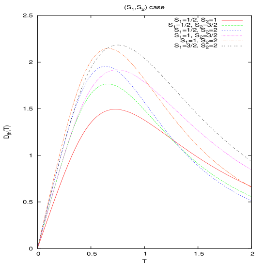
Figure 1: Thermal Drude weight $D_{th}(T)$ as function of temperature for $(S_{1}=1/2,S_{2}=1),(S_{1}=1/2,S_{2}=3/2),(S_{1}=1/2,S_{2}=2),(S_{1}=1,S_{2}=3/2),(S_{1}=1,S_{2}=2)$ and $(S_{1}=3/2,S_{2}=2)$.

These equations have a different driving term structure in comparison with those for the homogeneous case discussed in [7]. Therefore, the equations (26) constitute a new set of equations suitable for the description of the thermal Drude weight of the alternating spin chains.

Finally, the thermal Drude weight can be written as

$$D_{th}(T)=\beta^{2}\left\langle{{\cal J}^{(2)}}^{2}\right\rangle=\frac{1}{2}\beta^{2}\left(\frac{\partial}{\partial\lambda_{2}}\right)^{2}\left[\operatorname{ln}{\Lambda}^{(S_{1})}(0)+\operatorname{ln}{\Lambda}^{(S_{2})}(0)\right]\Big{|}_{\lambda_{2}=0}.$$ (28)

In Figure 1, we show numerical results for the thermal Drude weight as a function of temperature for specific choices of the spins $(S_{1},S_{2})$. At low temperatures the data exhibit a linear temperature dependence. The low-temperature asymptotics is accessible by an analytical treatment of the non-linear integral equations similar to [11]. From this we find that the thermal Drude weight $D_{th}(T)$ is generally a linear function of temperature and is proportional to the central charge of the system $c=\frac{3S_{1}}{S_{1}+1}+\frac{3(S_{2}-S_{1})}{(S_{2}-S_{1})+1}$[12]. Its explicit expression reads

$$D_{th}(T)\simeq\frac{\pi v_{s}c}{12}T,$$ (29)

where $v_{s}=2\pi$ is the sound velocity. These results are in agreement with those of the special case of homogeneous spin chains ($S_{1}=S_{2}=S$) [7].

The low-temperature asymptotics (29) is remarkable. This result may be derived on the hypothetical grounds of a particle picture of the thermal transport. If we assume that the elementary excitations of the system are the carriers of the thermal transport, we would expect that the thermal conductivity $\kappa$ of a system with finite mean free path $l$ (due to imperfections of the lattice) is $\kappa=v_{s}~{}c(T)~{}l$ where $v_{s}$ is the velocity of the elementary excitations and $c(T)$ is the specific heat. On the other hand, the existence of a finite mean free path defines a mean life time $\tau$ over which the Drude weight broadens to give a finite conductivity $\kappa=D_{th}~{}\tau$. The condition that both formulas agree is $D_{th}=v_{s}^{2}~{}c(T)$ which is –up to a numerical factor of order 1– equivalent to (29). It is remarkable that this reasoning yields the correct result despite the insufficient grounds: For generic Tomonaga-Luttinger liquids and conformally invariant field theories there are no delta-function peaks in the spectral function of the single-particle Green’s functions.

4 Conclusion

In this paper we have obtained a set of non-linear integral equations allowing for the explicit calculation of the thermal Drude weight for the integrable alternating ($S_{1},S_{2}$) spin chains. We have solved the equations numerically for specific values of $S_{1}$ and $S_{2}$. At low-temperatures we observe linear temperature dependence of the thermal Drude weight. This linear behavior is confirmed by the analytical low-temperature asymptotic solution showing that the coefficient of proportionality is the central charge of the system $c=\frac{3S_{1}}{S_{1}+1}+\frac{3(S_{2}-S_{1})}{(S_{2}-S_{1})+1}$. The existence of a non-zero Drude weight at finite temperature is a signature of anomalous thermal transport [2]. We hope our findings will be useful for experimental investigations of transport properties of quasi one-dimensional mixed spin systems, e.g [13].

Finally, we would like to remark that our results may be further generalized by including the alternation of an arbitrary number of different spins $S_{i},i=1,\dots,M$. Another direction of generalization would be the extension to anisotropic spin chains.

References

• [1] X. Zotos, Finite temperature Drude weight of the one-dimensional spin-1/2 Heisenberg model, 1999 Phys. Rev. Lett. 82 1764.
• [2] X. Zotos and P. Prelovsek, Transport in one dimensional quantum systems (review) in “Strong interactions in low dimensions”, series “Physics and Chemistry of Materials with Low Dimensional Structures”, eds. D. Baeriswyl and L. Degiorgi, Kluwer Academic Publishers p. 347-382 (2004); arXiv:cond-mat/0304630v2 .
• [3] J. Takeya, I. Tsukada, Y. Ando, T. Masuda and K. Uchinokura, Thermal conductivity of Mg-doped CuGeO3 at very low temperatures: Heat conduction by antiferromagnetic magnons, 2000 Phys. Rev. B 62 R9260; A.V. Sologubenko, K. Giannò, H.R. Ott, A. Vietkine and A. Revcolevschi, Heat transport by lattice and spin excitations in the spin-chain compounds SrCuO2 and Sr2CuO3, 2001 Phys. Rev. B 64 054412.
• [4] N. Hlubek, P. Ribeiro, R. Saint-Martin, A. Revcolevschi, G. Roth, G. Behr, B. Büchner, C. Hess, Towards ballistic heat transport in the S=1/2 Heisenberg chain compound $SrCuO_{2}$ arXiv:0908.1681
• [5] A.V. Sologubenko, T. Lorenz, H.R. Ott, A. Freimuth, Thermal conductivity via magnetic excitations in spin-chain materials, 2007 J. Low Temp. Phys. 147 387.
• [6] K. Sakai and A. Klümper, The thermal conductivity of the spin-1/2 XXZ chain at arbitrary temperature, 2002 J. Phys. A: Math. Gen. 35 2173; Non-dissipative thermal transport in the massive regimes of the XXZ chain, 2003 J. Math. A: Math. Gen. 36 11617.
• [7] G.A.P. Ribeiro and A. Klümper, Thermodynamics of antiferromagnetic alternating spin chains, 2008 Nucl. Phys. B 801 247.
• [8] P.P. Kulish, N.Y. Reshetikhin and E.K. Sklyanin, Yang-Baxter equation and representation theory-1, 1981 Lett. Math. Phys. 5 393.
• [9] H.J. de Vega, L. Mezincescu and R.I. Nepomechie, Thermodynamics of integrable chains with alternating spins, 1994 Phys. Rev. B 49 13223.
• [10] R. Kubo, Statistical-Mechanical theory of irreversible process -1: General theory and simple applications to magnetic and conduction problems, 1957 J. Phys. Soc. Japan 12 570.
• [11] J. Suzuki, Spinons in magnetic chains of arbitrary spins at finite temperatures , 1999 J. Phys. A: Math. Gen. 32 2341.
• [12] S.R. Aladim and M.J. Martins, Critical behaviour of integrable mixed-spin chains, 1993 J. Phys. A: Math. Gen. 26 L529.
• [13] O. Kahn, E. Bakalbassis, C. Mathoniere, M. Hagiwara, K. Katsumata, L. Ouahab, Metamagnetic Behavior of the Novel Bimetallic Ferromagnetic Chain Compound MnNi(NO2)4(en)2 (en=Ethylenediamine), 1997 Inorg. Chem. 36 1530; R. Feyerherm, C. Mathoniere and O. Kahn Magnetic anisotropy and metamagnetic behaviour of the bimetallic chain MnNi(NO2)4(en)2 (en = ethylenediamine), 2001 J. Phys.: Condens. Matter 13 2639.