Quantum Corrections to Multi-Quanta Higgs-Bags in the Standard Model

Abstract

We argue that the Standard Model contains stable bound states with a sufficiently large number $N$ of heavy quanta – top quarks $t,\bar{t}$ and gauge bosons $W,Z$ – of the form of collective “bags”, with a strongly depleted value of the Higgs VEV inside. More specifically, we study one-loop quantum corrections to a generic model of them, assuming “quanta” are described by a complex scalar field. We follow the practical formalism developed by Farhi et al. for the $N=1$ case, i.e. one particle in a bag, who found that for a very large Yukawa coupling the classical bags are destabilized by quantum effects. We instead study the problem with a coupling constant in the range of the Standard Model for a large number of quanta $N=50..5000$. We calculated both classical and one-loop effects and found that for such bags quantum corrections are small, of the order of a few percents or less.

I Introduction

Coherent bound states of a large number of bosonic quanta are known as “semiclassical solitons”. An important subclass of them – topological solitons – play a significant role in physics in general and in the dynamics of gauge theories in particular. Electroweak sphalerons, for instance, were extensively studied in the context of baryon number violation in the Standard Model (SM). Instantons drive the breaking of chiral $U(1)$ and $SU(N_{f})$ symmetries in QCD, while dyons/monopoles are believed to be related to the phenomenon of color confinement.

The objects we will study in this paper belong to the less famous subclass, namely “non-topological solitons”, which have remained somehow in the shadow of their topological relatives, although also studied – as pure theoretical constructions – for a long time. They are localized field configurations with finite energy which owe their existence not to topological properties, but rather to the existence of a conserved charge. The first examples were studied by R. Friedberg, T. D. Lee and A. Sirlin in Friedberg:1976me ; Lee:1991ax and some time later Coleman studied what he termed Q-balls Coleman:1985ki . These solitons, as we shall discuss below, are built out of scalar fields with an unbroken $U(1)$ symmetry. As is well known, Derrick’s theorem precludes the existence of time-independent soliton configurations in $d\gtr 1+1$ if only scalar fields are involved. However, non-topological solitons, both the Friedberg et al. and Q-balls, circumvent Derrick’s theorem by an explicit time dependence and owe their stability to the conserved charge associated to the unbroken $U(1)$. Despite of this similarity, they differ in some other respects. For instance, in the case of the Friedberg et al. type, there’s a second symmetry which is spontaneously broken due to the presence of a Higgs-like scalar field. They represent, as we shall see, regions of space in which the Higgs vacuum expectation value (VEV) is suppressed due to the presence of heavy particles. In this work we concentrate solely in this kind of Higgs-based solitons and the role of quantum corrections as we believe they might be relevant in applications to cosmology, although we will often compare our results to those previously obtained for Q-balls.

Regarding Q-balls, it was first shown in Coleman:1985ki that they exist in the limit of large charge $Q$, and it was later shown in Kusenko:1997ad that these classical Q-balls actually exist all the way down to $Q=1$. These small Q-balls may play an important role in cosmological applications Kusenko:1997ad and therefore it is important to determine the validity of the classical approximation. Therefore, the role of quantum corrections to these small Q-balls was explored in Graham:2001hr by using the methods developed in Farhi:1998vx and it was found that although they are small in comparison to the classical energy, they are comparable to the binding energy for small $Q$. It was finally concluded that quantum corrections (for typical values of coupling constants) render small Q-balls ($Q\lesssim 7$) unstable.

In contrast to all these works, we do not discuss hypothetical objects which can only appear in various extensions beyond the Standard Model, but address the range of stability and existence of the Multi-Quanta Higgs Bags (MQHB) in the SM itself. We have in mind the heaviest objects of the SM, top quarks $\bar{t},t$ and $W,Z$ bosons, to which we refer generically as “quanta”. Of course, bags with many top quarks, or $top-bags$ as we will call them, are quite different from scalar-quanta bags due both to their fermionic nature and their coupling to the Higgs field. However, these issues, and the potential role of these bags in the electroweak baryosynthesis problem, will be addressed elsewhere paperI ; paperII . In this work, which is mostly methodical in nature, we first address the issue of whether quantum corrections can or cannot destabilize these objects.

The interest in the issue originated from the question whether a sufficiently heavy SM-type fermion should actually exist as a different state, in which it depletes the Higgs VEV around itself and thus is accompanied by its own “bag” JS . Although classically this seemed to be possible, it was shown by Farhi et al. Farhi:2003iu that in fact quantum (one loop) effects destabilize such bags, except at such a large coupling that the theory itself is apparently sick, with an instability of its ground state. The issue rest dormant for some time till Nielsen and Froggatt Froggatt:2008ns argued that although the Yukawa coupling may still be small, there should be binding when the number of particles $N$ is such that

$$\frac{g^{2}}{4\pi}\ll 1,\,\,\,\frac{g^{2}}{4\pi}N>1.$$ (1)

Indeed, a similar generic argument explains for example why gravity, although very weak, can create bound states – planets and stars – but only for an “astronomically large” $N$.

These authors also suggested that 12 top+antitop quarks (the “magic number” corresponding to the maximal occupancy of the lowest $S_{1/2}$ orbital, 6 quarks and 6 anti-quarks with all spin and color values) already form deeply bound states with near-zero total mass. Here is when one of us (ES) became involved: in a paper with Kuchiev and Flambaum Kuchiev:2008fd we checked this suggestion and showed that, unfortunately, it is $not$ the case. While for a massless Higgs we found a weakly bound state of 12 tops, for a realistic Higgs mass there is no bound state at all. A possible direction to consider is that of introducing new hypothetical fermions with a stronger coupling (larger masses) than that of the top quark and the possibility of these forming baryons, well-bound by the Higgs. This issue has been discussed further in the second paper of the same authors Kuchiev:2008gt and we will discuss the implications of our study for this later.

Although we disagreed with the calculation by Nielsen and Froggatt Froggatt:2008ns on 12 tops, we think that further studies of multi-quanta Higgs bags are well justified. In this paper, we will be especially interested in the case in which the number of “quanta” $N$ is large enough to considerably modify the Higgs VEV compared to its vacuum value. In other words, we will focus on relativistic bound states, in which the “quanta” inside the soliton have masses quite different from their vacuum ones, rather than non-relativistic atom-like bound states with smaller $N$. This sector of the SM spectroscopy constitutes an interesting class of relativistic many-body systems, quite different from atoms and nuclei in many respects, especially regarding quantum corrections, which we study. While the experimental production of a large number of heavy quarks/bosons in a sufficiently small volume is clearly impossible, at the LHC or any other future proton accelerator, such states may play a significant role in cosmological baryogenesis at temperatures slightly below the electroweak phase transition paperII .

Turning now to the main subject of this paper; the role of quantum corrections to the energy of such configurations, we express their energy generically as a quantum loop diagram expansion

$$E(N)=E_{classical}\left[1+\sum_{k}C_{k}(N)(\frac{g^{2}}{4\pi})^{k}\right].$$ (2)

Below we calculate the one-loop coefficient $C_{1}$ closely following both the specific model and the practical methods developed in Farhi:1998vx . Very specifically, the issue we investigated is the $N$-dependence of the 1-loop radiative correction.

The paper is structured as follows. In Section II we formulate the Lagrangian and the “thin wall” approximation used to prove the existence of solitons at large enough $N$. In Section III we review the methods developed in Farhi:1998vx which provide a practical tool for numerically calculating the 1-loop radiative corrections to soliton configurations. It is important to note that these methods were designed for time-independent classical configurations while the non-topological configurations we just discussed have an explicit time dependence by having a non-zero $N$. However, as shown in Graham:2001hr (in an application to Q-balls) the method can easily be adapted to study a time-dependent configuration as well. After an estimate of the effect of quantum corrections in Section IV and a discussion of other secondary calculational details in Section V, we proceed to our results in Section VI.

II A classical soliton

Consider the action

$$S=\int d^{4}x\left(\frac{1}{2}(\partial_{\mu}\phi)^{2}-\frac{\lambda}{4!}(\phi^{2}-v^{2})^{2}+\left|\partial_{\mu}\psi\right|^{2}-g\psi^{\ast}\phi^{2}\psi\right)$$ (3)

where $\phi$ is a real scalar field, modeling the SM Higgs, with its VEV $\phi(r=\infty)=v$. A complex scalar field $\psi$ would have “quanta”, our simple version of $t,W$ and $Z$. This system was studied in Friedberg:1976me as an example which exhibits a soliton solution at the classical level. In this section we review the general arguments which were given in favor of the existence of these objects.

Due to the global symmetry $\psi\rightarrow e^{i\alpha}\psi$ in (3), there’s an associated conserved current, $\partial_{\mu}j^{\mu}=0,$ with

$$j_{\mu}=i\left(\psi^{\ast}\partial_{\mu}\psi-\psi\partial_{\mu}\psi^{\ast}\right)$$ (4)

and a corresponding conserved particle number

$$N=\int j^{0}d^{3}x.$$ (5)

Now, let the complex scalar be a time-dependent field rotating in internal space with a frequency $\omega$, i.e.

$$\psi(x,t)=e^{-i\omega t}\psi(x).$$ (6)

The classical energy $E_{cl}$ from (3) reads,

$$E_{cl}=\int d^{3}x\left[\frac{1}{2}(\vec{\nabla}\phi)^{2}+\left|\vec{\nabla}\psi\right|^{2}+\omega^{2}\left|\psi\right|^{2}\right.\\ \left.+\frac{\lambda}{4!}(\phi^{2}-v^{2})^{2}+g\phi^{2}\left|\psi\right|^{2}\right]$$ (7)

and from (5) we have

$$N=2\omega\int d^{3}x\left|\psi\right|^{2}.$$ (8)

The equations of motion read

$$-\omega^{2}\psi-\vec{\nabla}^{2}\psi+g\phi^{2}\psi = 0,$$ (9)

$$-\vec{\nabla}^{2}\phi-2g\left|\psi\right|^{2}\phi+\frac{\lambda}{6}(\phi^{2}-v^{2})\phi = 0.$$ (10)

By using the equation of motion (9) for $\psi$ in (7) and the expression (8) we find

$$E_{cl}=E_{h}+N\omega$$ (11)

with

$$E_{h}=\int d^{3}x\left[\frac{1}{2}\left|\vec{\nabla}h\right|^{2}+\frac{m^{2}}{8v^{2}}(h^{2}+2vh)^{2}\right],$$ (12)

where we have defined as usual $h\equiv\phi-v$. Therefore, the classic configuration consists of a static background field $h(x)$ and $N$ “quanta” of the $\psi$ field at an energy level $E_{0}=w$. In the Higgs vacuum, $\phi(r)=v$, $N$ quanta of the $\psi$ field would be forced to rest at the bottom of the continuum spectrum and the total energy of the system would simply be $NM$. However, in the background of a non-trivial Higgs field there are two competing effects. On the one hand, the gradient and potential terms in (12) increase the energy but, on the other hand, there might be some bound states levels with energy $0<E_{j}<M$ which can allocate the quanta, lowering the energy of the system of particles at the expense of creating such a Higgs configuration. In particular, if there’s a large region of nearly-zero Higgs VEV (where particles would be nearly massless), a soliton will be possible if the energy increase by creating such a region is offset by the energy decrease of $N$ particles giving away their mass.

Indeed, the existence of such solitons was shown in Friedberg:1976me by considering the following trial configuration: A time-independent Higgs field which vanishes inside a sphere of radius $R$ while outside it takes its asymptotic value, with a transition region of size $l$. The complex scalar $\psi(t,x)=e^{-i\omega t}\psi(x)$ is non-zero inside the sphere and vanishes outside. In a thin-wall approximation, $l\ll R,$ this provides a spherical well in which the complex field forms a relativistic bound state, i.e.

$$\begin{array}[]{c}\phi=0,\quad\psi(x,t)=e^{-i\omega t}\frac{A}{r}\sin(\omega r),\quad r\lesssim R,\\ \phi=v(1-e^{-(r-R)/l}),\quad\psi=0,\quad r\gtrsim R.\end{array}$$ (13)

with $\omega=\frac{\pi}{R}$. From (11), (12) the energy of such a configuration, in the limit of large $R$, reads

$$E=\frac{\pi N}{R}+\frac{\pi m^{4}}{2\lambda}R^{3}+O(R^{2}),$$ (14)

which has a minimum at

$$N\simeq\frac{3m^{4}R^{4}}{2\lambda},\quad E\simeq\frac{4\pi m}{3}\left(\frac{3}{2\lambda}\right)^{1/4}N^{3/4},$$ (15)

where $m^{2}=\lambda v^{2}/3$ and $M^{2}=gv^{2}$. Notice the power of $N$ with which the energy scales. If the Higgs field took its asymptotic value everywhere $($i.e. $\phi(r)=v)$, the total energy of the system would simply be given by $E=NM$. Since $E\propto N^{3/4}\ll N$ for large $N$, there’s always a large enough $N$ which makes the soliton configuration energetically favored over simply having $N$ particles in the Higgs vacuum. Notice that the critical configuration with $E_{c}=MN_{c}$ is given by

$$N_{c}\simeq\left(\frac{4\pi m}{3M}\right)^{4}\frac{3}{2\lambda}.$$ (16)

Since $R$ grows with $N$, this expression becomes more accurate for large $N$, i.e. when $M/m\rightarrow 0$ expression (16) gives the limiting value for $N_{c}$. It was similarly shown in Friedberg:1976me that in the limit $M/m\rightarrow\infty$, an upper bound on $N_{c}$ is given by

$$N_{c}<336\left(\frac{m}{M}\right)^{3}\frac{1}{\lambda}$$ (17)

and therefore when the Higgs becomes massless the solitons exist not only for large enough $N$ but actually all the way down to small $N$.

Recall that Derrick’s theorem precludes the existence of time- independent solitons with an action such as (3), but this no-go theorem is clearly circumvented here because of the explicit time dependence in (13), which leads to $N\sim\omega A^{2}$. If we had no time dependence the first term in (14) would vanish, rendering the system’s minimum at $R=0$, in accordance with Derrick’s theorem.

Although we have shown the existence of classical bags in certain approximations, in order to explicitly find such configurations with minimal energy we adopted a variational strategy. We first fix a smooth, 1-parameter, bag-shaped, background Higgs field ansatz on which we numerically solve the equation of motion for $\psi$. We then minimize the resulting energy with respect to the variational parameter. Once the classical solution is found we turn to the study of quantum corrections by implementing the method developed in Farhi:1998vx , which for completeness is reviewed in the next section.

III Quantum Corrections: Generalities

III.1 Time-independent configurations

As we have seen, a non-trivial Higgs background may create classical bag-like solitons. However, it also has a secondary effect at the quantum level, which is that of disrupting the energy levels of the vacuum by the Cassimir effect. To study whether this affects or not the existence of solitons we must study the vacuum energy, given to leading order in $\hbar$, by the effective action. The calculation of such an object will be plagued by the usual divergences of field theory and requires proper renormalization. In this section we review the method developed by Farhi et al. Farhi:1998vx , which precisely provides us a way of calculating the effective action in a manner consistent with on-shell mass and coupling renormalization. We shall consider the effective action induced only by integrating out fluctuations in $\psi$.

The one-loop effective action, induced by integrating out the $\psi$ field, is given by

$$e^{iS_{eff}[\phi]}=e^{iS_{\phi}}\frac{\int D\psi^{\ast}D\psi e^{iS_{\psi}}}{\int D\psi^{\ast}D\psi e^{\left.iS_{\psi}\right|_{V=0}}}$$ (18)

and the effective energy is then

$$E_{eff}=-\lim_{T\rightarrow\infty}\frac{1}{T}S_{eff},\quad S_{eff}=S_{cl}+S_{ct}-\log\det H$$ (19)

where $H$ is the quadratic operator $\frac{\delta^{2}S}{\delta\psi^{\ast}\delta\psi}$, generally of the form $H=-\square+M^{2}+V$. The matrix identity $\log\det H=Tr\log H$ allows us to write the effective action as a trace in functional space. We can perform this trace over a complete set of functions satisfying $H\psi_{\alpha}=0$ or

$$\left(-\nabla^{2}+M^{2}+V\right)\psi_{\alpha}=E_{\alpha}\psi_{\alpha}$$ (20)

which in the free ($V=0$) case are simply plane waves $e^{ikx}$. Therefore, in that case, $E_{vac.}^{\psi}\sim\int d^{4}k\log(k^{2}+M^{2})$ which by standard methods can be brought into the form $\int d^{3}k\sqrt{\vec{k}^{2}+M^{2}}=\int d^{3}k\left|E_{k}\right|$, which is the usual vacuum energy. In the presence of a background potential there might be, in addition to the continuum, some discrete levels corresponding to scattering bound states. In such case the vacuum energy generally reads

$$E_{vac.}^{{}_{\psi}}=\sumint_{\alpha}\left|E_{\alpha}\right|,$$ (21)

where $\alpha=\{i,k\}$ labels the discrete ($i$) eigenvalues, if any, and continuous ($k$) eigenvalues and $E_{\alpha}$ are the energies of the excitations. This is simply the sum of zero-point fluctuations $\frac{1}{2}\hbar w$ where the $\frac{1}{2}$ factor is absent due to $\psi$ being a complex field. Therefore, there are 3 contributions to the total effective energy given by

$$E[h]=E_{cl}[h]+E_{ct}[h]+E_{vac.}^{{}_{\psi}}[h],$$ (22)

where $E_{ct}$ is the necessary renormalization energy counterterm. For a fixed $h$, the spectrum consists of a continuous spectrum $E^{2}=k^{2}+M^{2}$ and (possibly) a finite number of bound states with energy $0<E_{j}<M$, i.e.

$$E_{vac.}^{{}_{\psi}}[h]=\sumint_{\alpha}E_{\alpha}=\sum_{j}E_{j}+\sum_{l}(2l+1)\int dk\rho_{l}(k)E(k)$$ (23)

where $\rho_{l}(k)$ is the density of states in momentum space and the $(2l+1)$ factor accounts for the degeneracy in the angular momentum projection. It can be shown that

$$\rho_{l}(k)=\rho_{l}^{0}(k)+\frac{1}{\pi}\frac{d}{dk}\delta_{l}(k)$$ (24)

where $\delta_{l}(k)$ is the scattering phase shift of the $l$’th partial wave under the potential $V(r)$ and $\rho_{l}^{0}(k)$ is the density of states in the absence of potential. Therefore, in order to calculate the whole 1-loop effective action we must calculate the phase shifts $\delta_{l}(k)$. As is standard in quantum mechanics, a Born approximation may be used. This represents an expansion in number of insertions of the potential $V(r)$ and in this model only diagrams with 1 and 2 insertions are divergent. Therefore, one defines the subtracted phase shift

$$\bar{\delta}_{l}(k)\equiv\delta_{l}(k)-\delta_{l}^{(1)}(k)-\delta_{l}^{(2)}(k)$$ (25)

where $\delta_{l}^{(1)}(k)$ and $\delta_{l}^{(2)}(k)$ are the first and second Born approximations to $\delta_{l}(k)$. It is shown in Farhi:1998vx that these two subtractions can be reintroduced into the action as divergent diagrams, which together with $E_{ct}[h]$ combine to give a finite contribution denoted by $\Gamma_{2}[h]$. Therefore, we have

$$E[h]=E_{cl}[h]+\Gamma_{2}[h]\\ +\frac{1}{\pi}\sum_{l}(2l+1)\int dk\left(\frac{d}{dk}\bar{\delta}_{l}(k)\right)E(k)+\sum_{j}\left|E_{j}\right|.$$ (26)

A very useful theorem due to Levinson states that the number of bound states $n_{l}$ with angular momentum $l$ in a given background potential is given by

$$n_{l}=\frac{1}{\pi}\left[\delta_{l}(0)-\delta_{l}(\infty)\right].$$ (27)

This allows us to partially integrate $d/dk$ in (26), picking up a boundary term $-M$ for each bound state, which finally gives an effective energy containing 4 terms, namely

$$E[h]=E_{cl}[h]+E_{bound}[h]+E_{cont.}[h]+\Gamma_{2}[h]$$ (28)

where

$$E_{bound}[h] = \sum_{j}(\left|E_{j}\right|-M),$$ (29)

$$E_{cont.}[h] = -\frac{1}{\pi}\sum(2l+1)\int_{0}^{\infty}dk\bar{\delta}_{l}(k)\frac{k}{\sqrt{k^{2}+M^{2}}},$$ (30)

and $E_{cl}$ is given by (11). Notice that after the boundary term due to Levinson’s theorem is included, the quantum correction due to the bound states is negative and therefore it lowers the total energy. This raises the possibility that one might find quantum solitons which classically are forbidden due to Derrick’s theorem. The existence of such solitons was explored in Farhi:1998vx with no success. From the previous discussions, however, we know that classical, time-dependent, soliton configurations exist for $N>0$ and we are interested in determining the effect of quantum corrections to these classical configurations.

III.2 Time-dependent configurations

We saw above that the method developed in Farhi:1998vx deals specifically with time-independent classical configurations. Therefore, to find the role of quantum corrections to the class of non-topological solitons we are interested in, we must adjust the methods to a time-dependent configuration. This has already been done in the case of $Q$-balls in Graham:2001hr by one of the same authors who developed the methods for the static case. In our case the same reasoning applies and we closely follow the same derivation. Nevertheless, as we shall discuss, in applying this method to the case at hand there’s an important difference with respect to Q-balls. The extension to the time-dependent case is easily carried out by studying fluctuations in a corotating frame. Let

$$\psi(x,t) = e^{-i\omega t}\left(\psi_{cl}(x)+\eta(x,t)\right),$$ (31)

$$\phi(x,t) = \phi_{cl}(x),$$ (32)

with $e^{-iwt}\psi_{cl}(x)$ the classical soliton discussed above and $\delta\psi=e^{-iwt}\eta(x,t)$ an arbitrary quantum fluctuation. Then the classical action reads

$$S_{cl}=\int d^{4}x\left[-\frac{1}{2}(\vec{\nabla}\phi_{cl})^{2}-\left|\vec{\nabla}\psi_{cl}\right|^{2}+\omega^{2}\psi_{cl}^{2}\right.\\ \left.-\frac{\lambda}{4!}(\phi_{cl}{}^{2}-v^{2})^{2}-g\left|\psi_{cl}\right|^{2}\phi_{cl}^{2}\right]$$ (33)

and to second oder in quantum fluctuations of $\psi$

$$S_{\eta}^{(2)}=\int d^{4}x\left[\left|(\partial_{0}-i\omega)\eta(x,t)\right|^{2}-\left|\vec{\nabla}\eta(x,t)\right|^{2}\right.\\ \left.-g\phi_{cl}^{2}\left|\eta(x,t)\right|^{2}\right].$$ (34)

Therefore,

$$-(\partial_{0}-i\omega)^{2}+\vec{\nabla}^{2}-g\phi_{cl}^{2}$$ (35)

is the quadratic operator of quantum fluctuations. For convenience, we parametrize $\eta(x,t)=e^{i(\omega-E)t}\eta(x)$, so that fluctuations over the static configuration $\left\{\phi_{cl}(x),\psi_{cl}(x)\right\}$ have an energy $E-\omega$ and hence their contribution to the effective energy is

$$E_{vac.}^{\psi}=\frac{1}{2}\sumint_{\alpha}\left|E_{\alpha}-\omega\right|,$$ (36)

where the $E_{\alpha}$’s are the solutions to the eigenvalue problem

$$\left(-E_{\alpha}^{2}-\vec{\nabla}^{2}+g\phi_{cl}^{2}\right)\eta_{\alpha}(x)=0,$$ (37)

i.e. we must study the zero modes of the operator $H=-E_{\alpha}^{2}-\vec{\nabla}^{2}+g\phi_{cl}^{2}$. Notice that we are left with a reduced problem which is identical to that we would of have to solve for the static case (20), with $V=g(h^{2}+2hv)\equiv g\chi$ and $M^{2}=gv^{2}$, but the contribution of each level is shifted by $\omega$. Now, since the spectrum in (37) is symmetric in $E\rightarrow-E$, we can write

$$E_{vac.}^{{}_{\psi}}[h]=\frac{1}{2}\sum_{E_{\alpha}>0}\left|E_{\alpha}-\omega\right|+\left|E_{\alpha}+\omega\right|=\sum_{E_{\alpha}>0}\max\{E_{\alpha},\omega\}.$$ (38)

As we shall see below,  if we only integrate out the fluctuations $\delta\psi$ from (3) we have $E_{\alpha}\geq\omega$ and therefore the vacuum energy is again simply

$$E_{vac.}^{{}_{\psi}}[h]=\sumint_{\alpha}\left|E_{\alpha}\right|$$ (39)

and the total energy reads

$$E=E_{cl}+\sum_{i}\left(\left|E_{i}\right|-M\right)+E_{cont.}+\Gamma_{2},$$ (40)

with $E_{cl}$ given by (11). To see that we have $E_{\alpha}\geq\omega$ in this case, we note that from the equations of motion we find $\left(-\omega^{2}-\vec{\nabla}^{2}+g\phi_{cl}^{2}\right)\psi_{cl}(x)=0$ in the $l=$ $0$ channel, which is the most tightly bound state and therefore the lowest positive energy is $E_{0}=\left|\omega\right|$, proving our assertion. It is important to note however that had we also considered fluctuations of the Higgs field as well, there would be a zero mode of the quadratic operator $H$ (which would be $2\times 2$) now in the $l=1$ channel, corresponding to translations of the soliton. This would imply that there’s an energy level $E_{0}$ below $\omega$ (in the $l=0$ channel), giving an additional contribution to the effective energy, namely $\omega-E_{0}$, with respect to (39). This is important in the case of the $Q$-ball where one has no other choice than considering such a zero mode as there’s only one field involved and actually this term dominates the whole quantum correction Graham:2001hr . This difference is important since this additional term, being positive, works against the stability of these solitons and is ultimately the responsible for rendering Q-balls with $Q\leq 7$, unstable. However, as just discussed, that’s not the case here due to the absence of the translational zero mode in the path integration.

IV Estimate of quantum corrections

Before going to the numerical calculations, we can illustrate the effects of quantum corrections on the solitons described in Section II by using the thin-wall construction. This configuration corresponds to a spherical potential well of depth $-gv^{2}=-M^{2}$ and size $R$, i.e. $V=-M^{2}\Theta(R-r)$, and the evaluation of the quantum corrections requires solving the energy levels of such a system. We wish to find the dependence of these energy levels on the size of the soliton. We can easily do this for the continuum energy relative to the Higgs vacuum. It is given by

$$E_{cont.}=\int d^{3}x\int d^{3}k\left[\sqrt{k^{2}+M^{2}+V}-\sqrt{k^{2}+M^{2}}\right]$$ (41)

and therefore

$$E_{cont.}=(4\pi)^{2}\int_{0}^{R}r^{2}dr\int dkk^{2}\left[k-\sqrt{k^{2}+M^{2}}\right].$$

The integral over $k$ is obviously divergent and requires proper regularization. However, the $R$-dependence is given by

$$E_{cont.}\sim R^{3}\sim N^{3/4}$$ (42)

and therefore it grows as the volume of the soliton and its effect is that of modifying the coefficient of $N^{3/4}$ in the classical energy (15). The precise dependence of the bound states’ contribution is harder to find analytically and will depend strongly on the coupling $g$, as this determines the depth of the potential $-gv^{2}$. Nevertheless, we can understand its main effect. We know that a spherical well of depth $-gv^{2}$ has a minimum size $R_{0}=\frac{\pi}{2v\sqrt{g}}$ at which the first bound state appears. For large coupling our potential becomes deeper and a large number of states could is bound. As is well known, in the case of an infinite spherical well there are an infinite number of bound states given by the spherical Bessel functions $j_{l}(kr)$. The boundary condition $j_{l}(kR)=0$ determines therefore the energy levels of a relativistic particle to be

$$E_{nl}=\frac{1}{R}\beta_{nl},$$ (43)

where $\beta_{nl}$ represents the $n$’th zero of the $l$’th order Bessel function. The number $n(R)$ of bound states in a finite potential well is finite and grows with $R$ and therefore the contribution (29) will be given by $n(R)(1/R-M)$, which may be significant at large $R$. Indeed, as we shall comment more later, for large enough coupling, it may become so negative that it wins over the classical energy of the soliton, making the vacuum unstable under the creation of empty bags of zero Higgs VEV. For relatively small values of $g$ ($\sim 1-3$) this term has the finite effect of lowering the number $N_{c}$ of particles required to have a stable configuration.

V Calculational Details

V.1 Variational method for classical solution:

Quantum corrections require some operations with the background Higgs field (such as finding its Fourier transform) which is difficult in practice to do for numerically generated shapes. Therefore we adopted a variational approach, in which the field is given in a simple analytic form, with certain parameters to be determined from energy minimization.

Our purpose is to find a variational minimum of (40). For this we used a family of 1-parameter Gaussian backgrounds for the Higgs

$$h(r)=-ve^{-r^{2}v^{2}/2w^{2}}$$ (44)

where $w>0$ is the variational parameter representing the size of the configuration. Notice that $\left\langle\phi\right\rangle\sim 0$ for $r\lesssim w$ while $\left\langle\phi\right\rangle\sim v$ for $r\gtrsim w$. As is customary, we refer to this configuration as a bag. It represents a region of size $\sim w$ of symmetric phase embedded in a space of broken phase. Inserting this ansatz into (12) gives us an analytical expression for the Higgs energy, which we denote $E_{bag}(w)$. Notice also that this profile for the Higgs provides an attractive potential $g\chi(r)$ under which the field $\psi$ scatters. By solving equation (37) with $l=0$ we find $\omega$, which is the lowest bound state level, henceforth denoted by $E_{0}$.

Recall that the energy of the soliton is given by

$$E(w)=E_{bag}(w)+NE_{0}(w).$$ (45)

For the energy to have a minimum we require that $(\delta E)_{N}=0$ and therefore

$$E_{bag}^{\prime}(w)+NE_{0}^{\prime}(w)=0$$ (46)

with ^′ denoting derivative w.r.t. $w$. This defines $N$ as a function of the bag’s size $w$ by

$$N(w)=-\frac{E_{bag}^{\prime}(w)}{E_{0}^{\prime}(w)}.$$ (47)

Furthermore, we must also have $E_{bag}^{{}^{\prime\prime}}(w)+NE_{0}^{{}^{\prime\prime}}(w)>0$. By taking the derivative of the first equation and noting that $E_{0}^{{}^{\prime}}<0$, we find

$$N^{\prime}(w)>0$$ (48)

to have a minimum. We are therefore interested to see if there’s a range for which $N^{\prime}(w)>0$ with $N$ given by (47).

V.2 Quantum Corrections

As explained in the Introduction we will follow here Farhi:1998vx , who developed a rather practical way to calculate the quantum correction, due to one-loop diagrams involving the “matter field” $\psi$, to the total energy of the system. It is given by several terms; the binding energy of the bound states, $E_{bound}$, the continuum term, $E_{cont.}$, representing regularized scattering phases, and the remaining regularized mass and charge renormalization, $\Gamma_{2}$.

To evaluate $E_{bound}$ we proceed as follows: Recall that $\delta_{l}(\infty)=0$ and therefore, according to Levinson’s theorem (27), the number of bound states with angular momentum $l$ is given by

$$n_{l}=\frac{1}{\pi}\delta_{l}(k=0).$$ (49)

According to Farhi:1998vx , from the radial equation of motion, one finds that the phase shifts are given by $\delta_{l}(k)=-2\Re\beta_{l}(k,r=0)$ with the $\beta_{l}$’s  satisfying

$$-i\beta_{l}^{{}^{\prime\prime}}-2ikp_{l}(kr)+2(\beta_{l}^{{}^{\prime}})^{2}+\frac{1}{2}g\chi(r)=0$$ (50)

where $p_{l}(x)\equiv d/dx\left(\ln\left[xh_{l}^{1}(x)\right]\right)$ and $h_{l}^{1}(x)$ is a spherical Hankel function and ^′ denotes derivative with respect to $r$. By solving this differential equation and taking the limit $k\rightarrow 0$ we found the number of bound states to be expected in every angular momentum channel at a given $w$. With this knowledge, we used a shooting method to find the energies of such states by solving the differential equation

$$\left(-\vec{\nabla}^{2}+g\phi_{cl}^{2}\right)\psi=E^{2}\psi.$$ (51)

That is, we repeatedly solved this differential equation for $\psi=\frac{u}{r}$ in a box of size $L=30$ for increasing values of $E$ from $0$ to $M$, with boundary conditions $u(0)=0$, $u^{\prime}(0)=1$. We then selected those solutions which vanish at infinity (i.e. $u(L)=0$), verifying that the number of such solutions matched those predicted by Levinson’s theorem.

To evaluate the continuum contribution (30), one must find the Born approximation to the phase shifts. These are similarly found by solving a set of coupled differential equations, which are detailed in the Appendix.

The calculation of the renormalization term $\Gamma_{2}$ is detailed in the Appendix and involves evaluating a double integral which is readily done numerically. It will be shown however that it is numerically suppressed to be several orders of magnitude smaller than the other contributions and may be neglected.

VI Results

We discuss the results of our numerical calculations starting with the lowest s-wave bound state. Its dependence on the bag size $w$ is shown in Fig. 1. The points represent the numerical results and the continuous line is an interpolation which, from (47), allowed us to find a smooth expression to be used below. Note that the curve does not go through the $w=0.9$ point, in which case there is no bound state: the point simply shows the mass of the quantum $outside$ the bag, $E_{0}=M=1$ for the coupling we use. Obviously, there’s a minimum bag size $w_{min}\sim 1$ at which the first state gets detached from the continuum to become a bound state with an energy just slightly below $M$. It is also clear that such shallow levels should be described by an atomic-like approach rather than by collective bags: we will not investigate their properties in this work, focusing only on deeper bound ones.

Table 1 shows some results for the energy of the bound states in different $l$-channels for different sizes of the bag. As we increase $w$, new levels appear and the energy of the lowest bound state approaches $0$. We also observe that the levels appear in the same order as in the spherical well potential (see, e.g. Landau ). For instance, for $w=7.9$ the order of the energy levels is $1s,$ $1p,$ $1d,$ $2s,$ $2p,$ $2d,$ $3s$.

$l/w$	$0.9$	$1.9$	$2.9$	$3.9$	$4.9$	$5.9$	$6.9$	$7.9$
$0$	$-$	$.809$	$\left.\begin{array}[]{c}.652\\ .997\end{array}\right.$	$\left.\begin{array}[]{c}.552\\ .892\end{array}\right.$	$\left.\begin{array}[]{c}.485\\ .803\end{array}\right.$	$\left.\begin{array}[]{c}.442\\ .745\end{array}\right.$	$\left.\begin{array}[]{c}.406\\ .710\end{array}\right.$	$\left.\begin{array}[]{c}.380\\ .682\\ .982\end{array}\right.$
$1$	$-$	$-$	$.857$	$.738$	$\left.\begin{array}[]{c}.652\\ .935\end{array}\right.$	$\left.\begin{array}[]{c}.596\\ .880\end{array}\right.$	$\left.\begin{array}[]{c}.552\\ .846\end{array}\right.$	$\left.\begin{array}[]{c}.515\\ .822\end{array}\right.$
$2$	$-$	$-$	$-$	$.886$	$.791$	$.725$	$\left.\begin{array}[]{c}.682\\ .977\end{array}\right.$	$\left.\begin{array}[]{c}.644\\ .951\end{array}\right.$
$3$	$-$	$-$	$-$	$-$	$-$	$-$	$-$	$-$

Table 1: This table shows a typical set of bound state levels in different angular momentum channels for different sizes of the bag with $g=\lambda=1$.

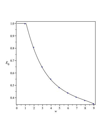
Figure 1: Energy of the lowest bound state as a function of $w$ for $g=\lambda=1$. The points show the results of our numerical calculations while the continuous line is an interpolation which allows us to find a smooth expression for $N$. We can see that there’s a minimal value $w_{min}\sim 1$ at which a bound state appears and its energy decreases smoothly to zero as $w$ increases. The number of levels in each channel coincides with those predicted by Levinson’s theorem.

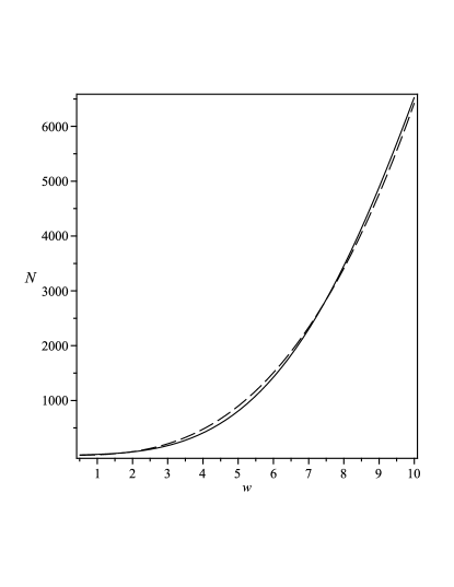
Figure 2: Number of particles necessary to extremize the energy of a configuration of bag’s size $w$. The number of particles to create a minimal bag is $\sim 20$, with a size $w_{min}\sim 1$. The dashed line represents the asymptotic behavior $\sim w^{2.86}$ for large $w$.

The number of quanta to bind in order to ensure that a bag of width $w$ has a saddle point is shown in Fig. 2. It continuously increases with $w$: as we showed in the previous section the condition $N^{\prime}(w)>0$ needs to be satisfied in order for the saddle point to be a local minimum and as we can see from the figure, this is always the case for $w>w_{min}$. By taking $g=\lambda=1$ in equation (16), we expect a stable soliton to be found for $N\simeq 51$. Indeed, our results in Fig. 3 show that without taking into account quantum corrections $N_{c}\simeq 52$ and the effect of quantum corrections is to lower $N_{c}$ to $\simeq 50$. Recall that we are ignoring the effect of the Higgs self-coupling at the quantum level and therefore $\lambda$ enters only in the expression for the classical energy. By taking $m/M\rightarrow 0$ (i.e. a BPS-like limit), the Higgs becomes massless and therefore the exchange forces between quanta become Coulombic. In this limit the minimum number of quanta $N_{c}$ to form a bound state is expected to be significantly decreased, as confirmed by equation (17). Notice also that this limit can be taken while keeping $g$, and therefore quantum corrections, small. Our numerical results for $\lambda=10^{-4}$ and $g=3$ are shown in Fig. 4. By further increasing the coupling $g$ while keeping $\lambda\simeq 0$ the size of the critical bag can be significantly decreased. For what we have seen, quantum corrections would not seem to spoil the existence of such small solitons but rather promote it, contrary to the case of Q-balls, due to the absence of the translational zero mode as discussed in §III.2.

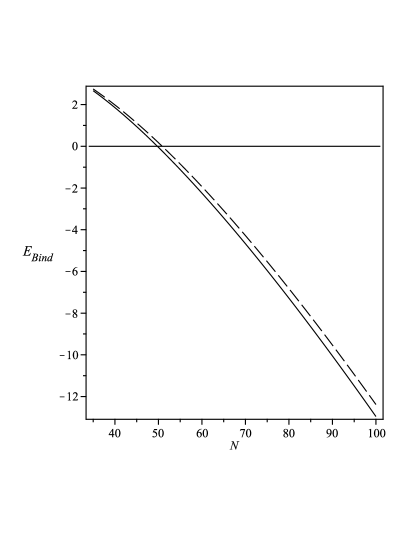
Figure 3: This figure shows the binding energy of the soliton with $g=1$ as a function of the number of particles. The solid line represents the binding energy including the quantum correction, while the dashed line contains only the classical energy. We can see that after a critical point $N_{c}\simeq 52$, it is energetically favorable to bind particles in a finite size bag rather than contracting the bag to zero size forcing the particles to migrate to the lowest state of the continuum spectrum with energy $NM$.

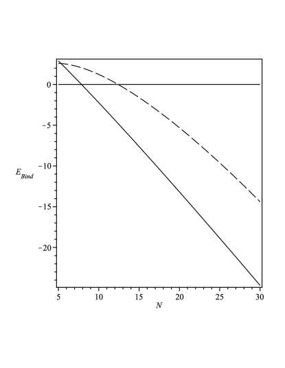
Figure 4: This figure shows the binding energy of the soliton with $\lambda=10^{-4}$ and $g=3$ as a function of the number of particles. Again, the dashed line is the classical binding energy while the solid line includes the quantum corrections. The number of particles to stabilize the bag is decreased by a smaller Higgs self-coupling and quantum corrections still favor the existence of such a soliton.

The vacuum energy, relative to the classical energy is embodied in the coefficient $C_{1}(N)$, which is shown in Fig. 5. Based on our discussion in Section IV, we expect $C_{1}(N)=\frac{4\pi}{g^{2}}\frac{E_{vac.}}{E_{cl.}}$ to behave as $a-\frac{b}{f(N)}$ for large $N$, with $a$ determined by the (renormalized) contribution from the continuum, while $b$ and $f(N)$ are determined by the bound-states contribution. Indeed, we found that our results up to $N\sim 6000$ are nicely fit by $a=1.64$, $b={2.04}$ and a very small power ${f(N)=N^{0.03}}$: A logarithmic fit is also possible. Since this plot is for $g^{2}/4\pi\approx.08$, we conclude that the one-loop coefficient $C_{1}$ in the generic expansion (2) grows slowly with $N$ and is asymptotically of order $1$. Therefore, even for the rather large coupling of top quarks ($g_{t}\approx 1$), quantum corrections seem to be under good theoretical control.

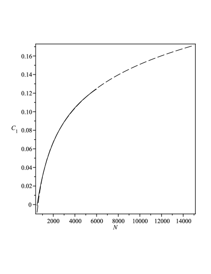
Figure 5: Coefficient $C_{1}(N)$ for $g=\lambda=1$. The dashed line represents an extrapolation of our results (solid line).

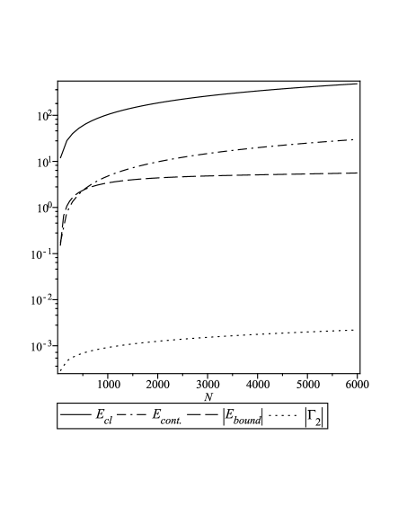
Figure 6: All $4$ contributions to the total energy in a log scale. $E_{bound}$ and $\Gamma_{2}$ are negative so their absolute values are shown. We can see that the main quantum correction for small solitons is given by $E_{bound}$ while for large solitons $E_{cont.}$ becomes the most relevant. The renormalization term $\Gamma_{2}$ is numerically suppressed by several orders of magnitude.

VII Summary and Discussion

The main content of the present paper is the explicit calculation of the regularized one-loop quantum correction to the energy of Multi-Quanta Higgs Bags, in a model in which “quanta” are represented by a charged scalar field. The main results are:
(i) For the range of couplings corresponding to the heaviest fermion (the top quark) and gauge bosons of the SM such bound states exist for $N$ larger than about 50;
(ii) quantum corrections to their energy is reasonably small, at the level of few percents at large $N$, although they play a larger role at smaller $N$, where they tend to $lower$ the binding boundary $N_{c}$. We do not think that the region close to it is under firm theoretical control, unlike the domain of large $N>100$.
(iii) For large solitons, the main quantum correction is given by the scattering states continuum, which grows with $N$ as the classical energy itself.
(iv) Even extrapolated to very large $N$ we find that the limits of validity of the perturbative expansion do include $g\approx 1$, i.e. the top quark of the SM.

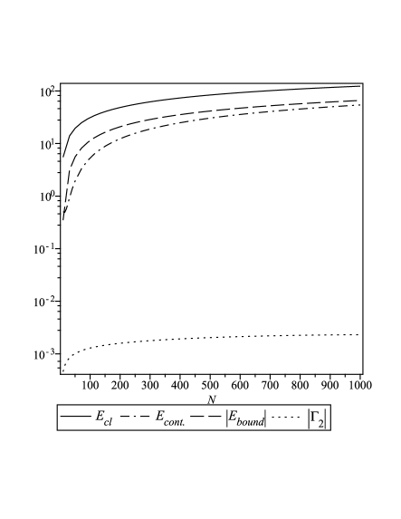
Figure 7: All $4$ contributions to the total energy for $g=3$. For larger coupling we can see how the contribution from $E_{bound}$ increases roughly an order of magnitude. It becomes comparable in magnitude to $E_{cont.}$ (although with the opposite sign) for large $N$ and dominant at small $N$.

As mentioned in the Introduction, the modification of the (quantum bound states and classical bag) calculation for fermions (real top quarks) and gauge bosons W,Z of the SM will be carried out elsewhere paperI , together with cosmological applications paperII .

As a remaining discussion issue, we may end up with the question when and what happens if the coupling is $larger$ than that of the top quark, namely $g>1$. It has been argued by Farhi et al. Farhi:1998vx that for sufficiently large $g$ the model becomes sick, because the vacuum itself (i.e. the $N=0$ state) becomes unstable against the spontaneous creation of large empty bags. Our experience with the large-coupling domain confirms it. A closer look at each contribution to the vacuum energy for larger $g$ uncovers the reason for this instability. From Figs. 6 and 7 we can discern the contribution to the total energy from each separate term in the effective energy for $g=1$ and $g=3$, respectively. For $g=1$ we observe that $\Gamma_{2}$ is numerically suppressed for all $N$ and the main quantum correction is due to an interplay between $E_{bound}$ and $E_{cont.}$, the former being dominant (and negative) for small $N$ ($\lesssim 100$), while the latter becomes dominant (and positive) for large $N$ and behaves similarly to the classical energy, as expected from our discussion in Section IV. Already for $g=3$ we found a significant increase in the contribution $E_{bound}$, which becomes comparable in magnitude (but opposite in sign) to the classical energy. Note that such coupling would correspond in the SM to fermions with a mass $\sim.5\,TeV$, and e.g. baryons made of such hypothetical fermions were suggested in Kuchiev:2008gt . We conclude that those states, if such fermions do exist, would have noticeable quantum corrections. Thus their theoretical status is much less solid than that of top-balls, perhaps asking for dedicated further study.

For $g\gtrsim 5$ the bound energy term under discussion becomes so negative that it completely compensates the classical energy of even an empty bag, therefore rendering the vacuum unstable. However, at such strong coupling the theory is in serious trouble and clearly beyond the range of validity of any perturbative expansion.

Acknowledgments. One author (ES) acknowledges an inspiring discussion with Prof. H. Nielsen, which triggered this project, as well as collaboration on a part of it with Profs. Flambaum and Kuchiev. This work was supported in part by the US-DOE grant DE-FG-88ER40388.

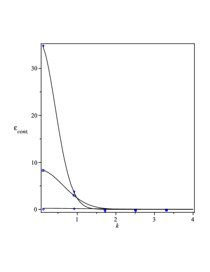
Figure 8: Typical $k$-dependence of the Born-subtracted continuum energy for $3$ values of increasing $w$ from the bottom up. The integral over $k$ grows quickly with increasing $w$.

Appendix

Here we summarize the equations needed for the calculation of the Born approximation to the phase shifts. This is needed for the explicit calculation of the continuum contribution. We denote the first and second Born terms by $\delta_{l1}$ and $\delta_{l2}$. A series expansion in powers of $g$ for the phase shifts may be written as

$$\beta_{l}=g\beta_{l1}+g^{2}\beta_{l2}+...$$ (52)

with $\delta_{l1}=-2gRe\beta_{l1}(k,r=0)$ and $\delta_{l2}=-2g^{2}Re\beta_{l2}(k,r=0)$ and $\beta_{l1,2}$ satisfy the set of coupled differential equations

$$-i\beta_{l1}^{{}^{\prime\prime}}-2ikp_{l}(kr)\beta_{l1}^{{}^{\prime}}+\frac{1}{2}\chi(r) = 0,$$ (53a)

$$-i\beta_{l2}^{{}^{\prime\prime}}-2ikp_{l}(kr)\beta_{l2}^{{}^{\prime}}+2(\beta_{l1}^{{}^{\prime}})^{2} = 0.$$ (53b)

The continuum contribution is given by

$$E_{cont.}=\int_{0}^{\infty}\varepsilon_{cont.}(k)dk,$$ (54)

with

$$\varepsilon_{cont.}(k)=-\frac{1}{\pi}\sum_{l}(2l+1)\bar{\delta}_{l}(k)\frac{k}{\sqrt{k^{2}+M^{2}}}$$ (55)

and $\bar{\delta}_{l}(k)\equiv\delta_{l}(k)-\delta_{l}^{(1)}(k)-\delta_{l}^{(2)}(k)$. Each of these terms is given as a solution to the set of differential equations (50) and (53). In figure (8) we show the continuum energy $\varepsilon_{cont.}$ as a function of $k$ for 3 increasing values of $w$ from the bottom up. It can be seen that the Born subtracted $\delta_{l}$ is rapidly convergent in $k$ and that the integral grows quickly with $w$.

The renormalization effect, encoded in $\Gamma_{2}$ is calculated from a set of Feynman diagrams and is given by

$$\Gamma_{2}=\frac{g^{2}}{(4\pi)^{2}}\int\frac{q^{2}}{2\pi^{2}}dq\int_{0}^{1}dx\left\{-\frac{4x(1-x)v^{2}q^{2}}{M^{2}-m^{2}x(1-x)}h(q)^{2}\right.\\ \left.+\left[\log\frac{M^{2}+q^{2}x(1-x)}{M^{2}-m^{2}x(1-x)}-\frac{m^{2}x(1-x)}{M^{2}-m^{2}x(1-x)}\right]\chi(q)^{2}\right\}$$ (56)

where $\chi(q)$ and $h(q)$ are the spatial Fourier transforms of $\chi(x)$ and $h(x)$. Notice that there are numerical factors $(4\pi)^{4}$ in the denominator, which suppresses this contribution with respect to the other ones. See Farhi:1998vx for more details.

References

- (1) R. Friedberg, T. D. Lee and A. Sirlin, Phys. Rev. D 13, 2739 (1976).
- (2) T. D. Lee and Y. Pang, Phys. Rept. 221, 251 (1992).
- (3) S. R. Coleman, Nucl. Phys. B 262, 263 (1985) [Erratum-ibid. B 269, 744 (1986)].
- (4) A. Kusenko, Phys. Lett. B 404, 285 (1997) [arXiv:hep-th/9704073].
- (5) N. Graham, Phys. Lett. B 513, 112 (2001) [arXiv:hep-th/0105009].
- (6) E. Farhi, N. Graham, P. Haagensen and R. L. Jaffe, Phys. Lett. B 427, 334 (1998) [arXiv:hep-th/9802015].
- (7) Marcos P. Crichigno, M. Y. Kuchiev, V. V. Flambaum and E. Shuryak, Multiquanta Bound States of the Standard Model., in preparation.
- (8) M. Y. Kuchiev, V. V. Flambaum and E. Shuryak, Multiquanta Bound States of the Standard Model. II.Big Bang Baryogenesis, in preparation.
- (9) R. Johnson and J. Schechter, Phys. Rev. D36 (1987) 1484.
- (10) E. Farhi, N. Graham, R. L. Jaffe, V. Khemani and H. Weigel, Nucl. Phys. B 665, 623 (2003) [arXiv:hep-th/0303159].
- (11) C. D. Froggatt, L. V. Laperashvili, R. B. Nevzorov, H. B. Nielsen, and C. R. Das, (2008), 0804.4506; C. D. Froggatt and H. B. Nielsen, Surveys High Energ. Phys. 18, 55 (2003), hep-ph/0308144; C. D. Froggatt, H. B. Nielsen, and L. V. Laperashvili, Int. J. Mod. Phys. A20, 1268 (2005), hep-ph/0406110.
- (12) M. Y. Kuchiev, V. V. Flambaum and E. Shuryak, Phys. Rev. D 78, 077502 (2008) [arXiv:0808.3632 [hep-ph]].
- (13) M. Y. Kuchiev, V. V. Flambaum and E. Shuryak, “Light bound states of heavy fermions,” arXiv:0811.1387 [hep-ph].
- (14) R. MacKenzie, F. Wilczek, and A. Zee, Phys. Rev. Lett. 53, 2203 (1984).
- (15) J. Schwinger, Phys. Rev. 94 (1954) 1362.
- (16) Landau Lifshitz. Quantum Mechanics, Non-Relativistic Theory (1958).