Extracting the fundamental parameters

Abstract

If supersymmetry is discovered at the LHC, the extraction of the fundamental parameters will be a formidable task. In such a system where measurements depend on different combinations of the parameters in a highly correlated system, the identification of the true parameter set in an efficient way necessitates the development and use of sophisticated methods. A rigorous treatment of experimental and theoretical errors is necessary to determine the precision of the measurement of the fundamental parameters. The techniques developed for this endeavor can also be applied to similar problems such as the determination of the Higgs boson couplings at the LHC.

1 INTRODUCTION

In the following two scenarios for the extraction of the fundamental parameters from experimental data will be discussed. The first example is vintage supersymmetry as an example for the precision achievable at the LHC when supersymmetry provides a multitude of signatures. The second example is difficult supersymmetry, be it that most, but not all of the supersymmetric partners are not observed, or that only a light Higgs boson is observed and its properties measured at the LHC.

In a supersymmetric theory, each fermionic degree of freedom has a bosonic counter part and vice versa. Squarks, sleptons, neutralinos and charginos are the partners of the quarks, leptons, neutral and charged gauge and Higgs bosons. Supersymmetric theories have “no” problems with radiative corrections, they predict a light Higgs boson with a mass less than 150 GeV, provide interesting phenomenology at the the TeV scale and may provide a link to the Planck scale.

Many different models describe the phenomenology of supersymmetry. In the following sections, three of these will be discussed: mSUGRA as an example of a model with few parameters, most of which are defined at the grand unification scale (GUT), Decoupled Scalars Supersymmetry (DSS) as an example where a part of the supersymmetric spectrum is unobservable at the LHC, and the MSSM as a an example of a model defined at the electroweak scale with many parameters. Determining this model (in contrast to mSUGRA) may allow to measure grand unification of the supersymmetric breaking parameters.

R–parity is conserved in the following thus supersymmetric particles (cascade-)decay to the lightest supersymmetric particle (LSP). In the following the lightest neutralino will play the role of the LSP. It is stable, neutral and weakly interacting. The LSP is a candidate for dark matter. The experimental signature for supersymmetry at colliders is missing transverse energy due to the presence of the undetected LSP(s).

In the present absence of supersymmetric signals it is necessary to define benchmark points in order to study the potential of supersymmetry discovery and measurement. The reference point SPS1a [1] has been studied intensely in the past years in LHC as well as ILC simulations [2]: In SPS1a gluinos and squarks have masses of the order of 500–600 GeV, light sleptons have masses of 150 GeV and the Higgs boson is at the LEP limit.

2 DETERMINATION OF PARAMETERS

The difficulties of determining the fundamental parameters from measurements can be illustrated by taking mSUGRA as an example. The mass of the smuon depends on m₀, m_1/2 and $\tan\beta$. The mass of the chargino depends on m_1/2 and $\tan\beta$, thus the same parameter has an impact on different measurements. Additionally the experimental errors can be correlated and each theoretical prediction also has an error associated to it. Thus in order to disentangle the system to obtain the best possible precision on all parameters, a global Ansatz is necessary.

For each observable in addition to a precise “experimental” determination, a precise theory prediction must be associated. This means the most up to date calculations for masses, branching ratios, cross sections as well as dark matter predictions have to be used. A summary of different tools is listed in [3].

The first study of this type was performed in [4]. The Fittino [5] and SFitter [6, 7] collaborations studied the reconstruction of parameters with sophisticated techniques which will be described later.

3 PREDICTIONS FROM PRESENT DATA

While no direct observation of a supersymmetric particle is available, the theoretical predictions of precision observables are sensitive, via radiative corrections, to the parameters of supersymmetry. A wealth of precise measurements such as the mass of the W boson and the top quark mass have been made at LEP [8] and the TeVatron [9]. Additionally precise measurements in the b–sector, such as the branching ratio of b$\rightarrow$s$\gamma$ have been performed. The anomalous magnetic moment of the muon ($(g-2)_{\mu}$) is known with very good precision and WMAP has provided a measurement of the relic density.

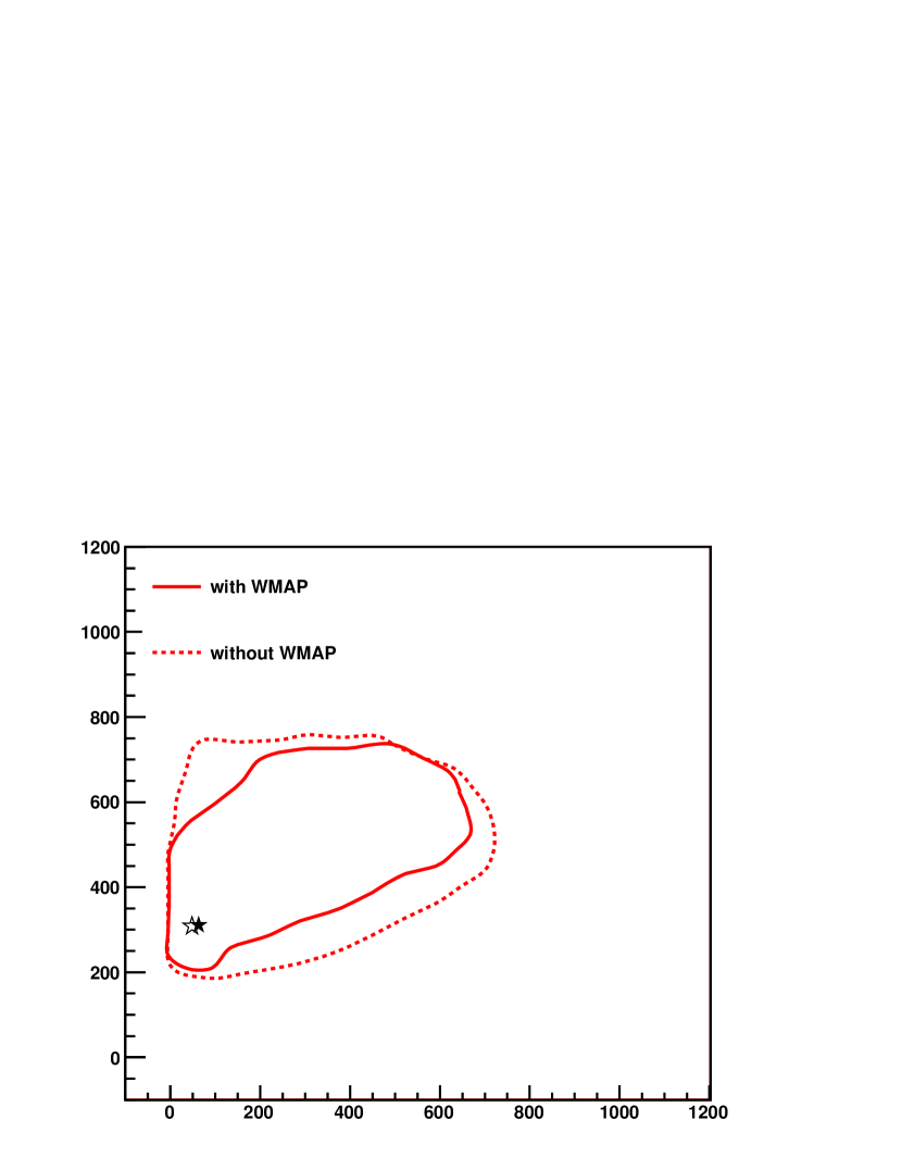
Figure 1: The best fit result is shown in the $(\mathrm{m}_{1/2}/\mathrm{m}_{0})$ plane as well as the contours including and excluding the WMAP measurements.

The comparison of the predictions with the measurements allows to determine the parameters of mSUGRA [10]. Figure 1 shows the best–fit point in the $(\mathrm{m}_{1/2}/\mathrm{m}_{0})$ plane. Due to $(g-2)_{\mu}$ a positive sign of $\mu$ is favored. It is intriguing to note that the SPS1a point, a point considered to be overly optimistic at the time of its definition, is close to the best–fit point.

This approach can be taken a step further by fitting the phenomenological MSSM, a weak scale model with about 20 supersymmetric parameters. Using a Bayesian approach with a linear prior and a logarithmic prior, one can infer on the MSSM parameters as shown in [11]. The dependence of the results on the prior should disappear as more information (such as supersymmetric mass measurements) become available. It is interesting to note that in this study the preference for a positive sign of the $\mu$ parameter from the muon anomalous magnetic moment is not observed.

4 VINTAGE SUPERSYMMETRY

Table 1: LHC measurements [2] in SPS1a are shown. The nominal values are calculated with SuSpect. Statistical errors, systematic errors from the lepton (LES), jet energy scale (JES) and theoretical errors are all given in GeV.

type of		nominal	stat.	LES	JES	theo.
measurement		value	error
$m_{h}$		108.99	0.01	0.25		2.0
$m_{t}$		171.40	0.01		1.0
$m_{\tilde{l}_{L}}-m_{\chi_{1}^{0}}$		102.45	2.3	0.1		2.2
$m_{\tilde{g}}-m_{\chi_{1}^{0}}$		511.57	2.3		6.0	18.3
$m_{\tilde{q}_{R}}-m_{\chi_{1}^{0}}$		446.62	10.0		4.3	16.3
$m_{\tilde{g}}-m_{\tilde{b}_{1}}$		88.94	1.5		1.0	24.0
$m_{\tilde{g}}-m_{\tilde{b}_{2}}$		62.96	2.5		0.7	24.5
$m_{ll}^{\mathrm{max}}$:	three-particle edge($\chi_{2}^{0}$,$\tilde{l}_{R}$,$\chi_{1}^{0}$)	80.94	0.042	0.08		2.4
$m_{llq}^{\mathrm{max}}$:	three-particle edge($\tilde{q}_{L}$,$\chi_{2}^{0}$,$\chi_{1}^{0}$)	449.32	1.4		4.3	15.2
$m_{lq}^{\mathrm{low}}$:	three-particle edge($\tilde{q}_{L}$,$\chi_{2}^{0}$,$\tilde{l}_{R}$)	326.72	1.3		3.0	13.2
$m_{ll}^{\mathrm{max}}(\chi_{4}^{0})$:	three-particle edge($\chi_{4}^{0}$,$\tilde{l}_{R}$,$\chi_{1}^{0}$)	254.29	3.3	0.3		4.1
$m_{\tau\tau}^{\mathrm{max}}$:	three-particle edge($\chi_{2}^{0}$,$\tilde{\tau}_{1}$,$\chi_{1}^{0}$)	83.27	5.0		0.8	2.1
$m_{lq}^{\mathrm{high}}$:	four-particle edge($\tilde{q}_{L}$,$\chi_{2}^{0}$,$\tilde{l}_{R}$,$\chi_{1}^{0}$)	390.28	1.4		3.8	13.9
$m_{llq}^{\mathrm{thres}}$:	threshold($\tilde{q}_{L}$,$\chi_{2}^{0}$,$\tilde{l}_{R}$,$\chi_{1}^{0}$)	216.22	2.3		2.0	8.7
$m_{llb}^{\mathrm{thres}}$:	threshold($\tilde{b}_{1}$,$\chi_{2}^{0}$,$\tilde{l}_{R}$,$\chi_{1}^{0}$)	198.63	5.1		1.8	8.0

The point SPS1a provides a vast number of measurements at the LHC. In particular, the long cascade decay $\tilde{q}_{L}\rightarrow\chi_{2}^{0}q\rightarrow\tilde{\ell}_{R}\ell q\rightarrow\ell\ell q\chi^{0}_{1}$ can be observed well above the Standard Model and supersymmetric backgrounds. The final state consists of opposite-sign same flavor leptons, i.e., electrons and muons, and hard jets. In this decay chain edges and thresholds can be measured by reconstructing invariant masses of different combinations: lepton–lepton, lepton–jet, lepton–lepton–jet. These endpoints are analytical functions of the masses of the particles, they do not depend on the underlying theoretical model.

The results of the LHC study assuming an integrated luminosity of 300 fb^-1 are shown in Table 1. Several of the measurements are limited by the systematic error on the energy scale, which is assumed to be of the order of percent for jets and at the per mil level for leptons. Using the kinematic formula for the edges and endpoints, the absolute masses of the supersymmetric particles can be determined. This procedure, usually performed with fits on toy experiments introduces additional correlations. For the determination of the fundamental parameters it is therefore preferable to start directly from the edges and thresholds. Simplifying the results of the analysis for the ILC, as soon as the particles are kinematically accessible, they can be measured an order of magnitude more precisely than at the LHC.

4.1 mSUGRA

Two issues have to be addressed to determine the fundamental parameters from the experimental measurements: finding the true/correct parameter set from a strongly correlated system of measurements and determining accurately the errors on the parameters.

For the first issue several different techniques have been developed to efficiently sample a multi dimensional parameter space. Fittino [5] has developed the technique of simulated annealing, which allows to cross potential boundaries. These boundaries could confine a simple fit based search to secondary minima. SFitter [6, 7] has developed weighted Markov chains which have the advantage of efficient sampling in high dimensions. Markov chains are linear in the number of parameters in contrast to a simple grid based approach where all parameters are sampled with a predefined step size.

Table 2: Expected errors on the mSUGRA parameters at the LHC and ILC. Flat theory errors are used.

	SPS1a	$\Delta_{\rm endpoints}$	$\Delta_{\rm ILC}$	$\Delta_{\rm LHC+ILC}$	$\Delta_{\rm endpoints}$	$\Delta_{\rm ILC}$	$\Delta_{\rm LHC+ILC}$
		exp. errors			exp. and theo. errors
$m_{0}$	100	0.50	0.18	0.13	2.17	0.71	0.58
$m_{1/2}$	250	0.73	0.14	0.11	2.64	0.66	0.59
$\tan\beta$	10	0.65	0.14	0.14	2.45	0.35	0.34
$A_{0}$	-100	21.2	5.8	5.2	49.6	12.0	11.3
$m_{t}$	171.4	0.26	0.12	0.12	0.97	0.12	0.12

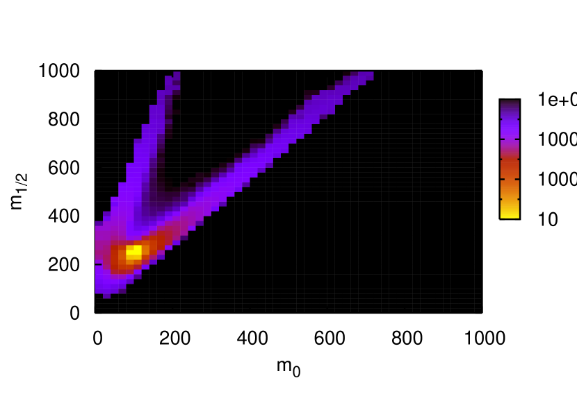
Figure 2: The result of the profile likelihood in the $(\mathrm{m}_{1/2}/\mathrm{m}_{0})$ plane is shown [7]. The best–fit point is clearly identified and corresponds to the true SPS1a parameter set.

After having produced a full dimensional exclusive likelihood map, two types of projections are possible to reduce the number of parameters, e.g., to illustrate correlations between two parameters. The Bayesian approach introduces a measure but conserves the property of probability density in the projection. The frequentist approach uses a profile likelihood which ensures that the absolute minimum is always retained in the projection. In illustration of a two dimensional correlation plot is shown in Figure 2 for the frequentist approach in mSUGRA. The correct parameter set was found from the measurements.

The Markov chains also allow to identify secondary minima. Even in a tightly constrained model such as mSUGRA secondary minima occur. In particular, when in addition to the fundamental parameters the Standard Model parameters are also allowed to vary within their experimental error. SFitter showed [7] that the interplay of the top quark mass and the tri–linear coupling can lead to additional solutions. However these can be discarded easily by comparing the $\chi^{2}$ value of the solutions which are much larger than for the correct parameter set.

To address the second issue, determination of the errors on the parameters, one can either determine them in a single fit using for example MINOS or by using toy-experiments, i.e., performing the parameter determination for a large number of datasets which have been smeared according to the experimental and theoretical errors. In the latter case the width (RMS or a Gaussian fit) of the distribution of the central value of the fits is the error. This procedure is more robust than a single fit and used most of the time, especially in the presence of correlations.

While the experimental errors can usually be treated as Gaussian with well defined correlations, e.g., the energy scale error is fully correlated among measurements, the theoretical error deserves special attention. Here the RFit [12] approach is followed. Within the theoretical error, the contribution to the $\chi^{2}$ is zero. Beyond this region the usual $\chi^{2}$ contribution calculated with the experimental error is used. The procedure ensures that no particular value within the theoretical error region is privileged. The typical theoretical errors used for this study are 3% for strongly interacting particles (squarks and gluinos) and 1% for weakly electromagnetically interacting particles (sleptons, neutralinos and charginos). In the Higgs sector an error of 2 GeV is used.

The results are summarized in Table 2 for the LHC, ILC, the combination of LHC and ILC with and without theoretical errors. The precision of the LHC alone is at the level of percent for the determination of the parameters. It is improved by the ILC by about an order of magnitude. Including the theoretical errors has an impact on the precision at both machines, the errors are larger by a factor of three to four. Thus the precision of the parameter determination at the LHC is limited by the precision of the theoretical predictions. The SPA project [13] aims to improve the situation. It is also important to note that at the LHC the precision on the top quark mass of 1 GeV has an impact of about 10% on the precision of the determination of the parameters.

4.2 MSSM

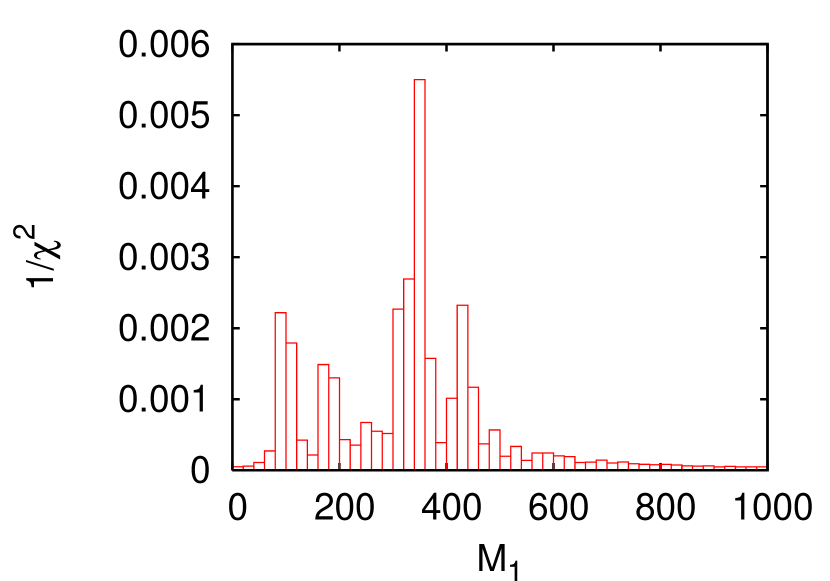
Figure 3: The result of the profile likelihood for the gaugino mass parameter $\mathrm{M}_{1}$ is shown [7]. Several peaks are identified corresponding to secondary maxima.

The search for the global minimum is more complex in the MSSM where more parameters have to be determined. If the unification of the first and generation sfermions is not assumed, 19 parameters have to be determined. A complex mix of different techniques has to be applied: markov chains and a gradient search to refine the resolution of the minima. The result of the profile likelihood procedure at the LHC is shown in Figure 3 for the gaugino mass parameter $\mathrm{M}_{1}$.

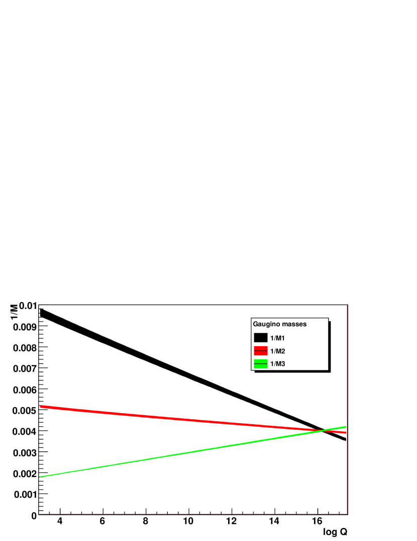
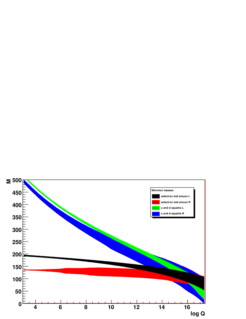
Figure 4: Top: Extrapolation of the inverse of the gaugino mass parameters to the GUT scale for two of the degenerate solutions at the LHC. Grand unification is observed in one case corresponding to the correct parameter set (left), but not in the other solution (right). M₁ is in black, M₂ red and M₃ is in green. Bottom: Extrapolation of the first and second generation scalar mass parameters to the GUT scale for two of the degenerate solutions. Grand unification is observed in one case (left) corresponding to the correct SPS1a MSSM parameter set, but not the other one (right).

Several secondary minima are observed. They cannot be distinguished by their $\chi^{2}$ value which is identical in all cases. The degeneracy of the eight secondary minima can be understood qualitatively by analyzing the gaugino–Higgsino sector. At the LHC in SPS1a only three neutralinos can be measured according to the studies available today, but the sector is determined by four parameters M₁, M₂, $\mu$ and $\tan\beta$, neglecting radiative corrections. The system is therefore under-constrained. Additionally M₁ and M₂ can be exchanged without a change in the LHC observables. The situation is improved dramatically when the ILC measurements are added as they complete the neutralino sector and add the masses of the charginos providing additional constraints to determine the MSSM parameters without ambiguity.

The MSSM is defined at the electroweak scale. The definition of its parameters does not depend on the model of supersymmetry breaking. Thus, having determined the parameters at the weak scale, the extrapolation of the parameters to the GUT scale can be performed. Instead of assuming unification at the GUT scale as in mSUGRA, it can now be tested. As eight degenerate solutions have been determined the extrapolation is performed for each one of them. Two examples are shown in Figure 4 (top). Figure 4 (top left) corresponds to a solution which is the correct SPS1a MSSM parameter set. GUT unification of the gaugino masses is observed as expected. However in Figure 4 (top right) GUT unification is not observed. Of the eight degenerate solutions only one unifies the gaugino masses at the GUT scale, one almost does (this corresponds to the parameter set where only the sign of $\mu$ is changed with respect to SPS1a) and the six other solutions clearly do not unify.

In addition to the gaugino sector the extrapolation of the scalar sector in the first two generations can also be studied at the LHC. The third generation is under-constrained due to the lack of measurements in the stop sector. In Figure 4 (bottom) the extrapolation is shown on the left for the correct SPS1a MSSM parameter set and on the right for the same set with the exception of the stau parameter which has been moved far from the true solution (the $\chi^{2}$ values are identical). Unification can be observed in the first case, but not in the second one, while the gaugino unification is observed in both cases. This can be understood from the RGE equations. The RGEs in the gaugino sector essentially decouple, whereas in the RGEs of the scalar sector for a parameter all other parameters. A bad measurement, i.e., far from its true value, therefore has a large impact on the extrapolation of all scalar parameters. The extrapolation is stabilized by the measurements of the ILC. The combination of LHC and ILC therefore will allow to measure grand unification of all supersymmetric parameters, whereas for the LHC, without further measurements, one can only observe that one of the ambiguous solutions is compatible with GUT unification.

4.3 RELIC DENSITY

Table 3: Signatures included in the Higgs coupling analysis for a Higgs mass of 120 GeV and an integrated luminosity of 30 fb^-1. The factor after the background rates describes how many events are used to extrapolate into the signal region. The last two columns give the one-sigma experimental and theory error bars on the signal.

production	decay	$S+B$	$B$		$S$	$\Delta S^{\mathrm{(exp)}}$	$\Delta S^{\mathrm{(theo)}}$
$gg\to H$	$ZZ$	13.4	6.6	($\times$ 5)	6.8	3.9	0.8
$qqH$	$ZZ$	1.0	0.2	($\times$ 5)	0.8	1.0	0.1
$gg\to H$	$WW$	1019.5	882.8	($\times$ 1)	136.7	63.4	18.2
$qqH$	$WW$	59.4	37.5	($\times$ 1)	21.9	10.2	1.7
$t\bar{t}H$	$WW(3\ell)$	23.9	21.2	($\times$ 1)	2.7	6.8	0.4
$t\bar{t}H$	$WW(2\ell)$	24.0	19.6	($\times$ 1)	4.4	6.7	0.6
inclusive	$\gamma\gamma$	12205.0	11820.0	($\times$ 10)	385.0	164.9	44.5
$qqH$	$\gamma\gamma$	38.7	26.7	($\times$ 10)	12.0	6.5	0.9
$t\bar{t}H$	$\gamma\gamma$	2.1	0.4	($\times$ 10)	1.7	1.5	0.2
$WH$	$\gamma\gamma$	2.4	0.4	($\times$ 10)	2.0	1.6	0.1
$ZH$	$\gamma\gamma$	1.1	0.7	($\times$ 10)	0.4	1.1	0.1
$qqH$	$\tau\tau(2\ell)$	26.3	10.2	($\times$ 2)	16.1	5.8	1.2
$qqH$	$\tau\tau(1\ell)$	29.6	11.6	($\times$ 2)	18.0	6.6	1.3
$t\bar{t}H$	$b\bar{b}$	244.5	219.0	($\times$ 1)	25.5	31.2	3.6
$WH/ZH$	$b\bar{b}$	228.6	180.0	($\times$ 1)	48.6	20.7	4.0

At this point all supersymmetric parameters have been determined, therefore the complete particle spectrum can be deduced. From the spectrum and its couplings the relic density is predicted [14]. Neglecting the theoretical error and performing the analysis in mSUGRA, a precision of about 2% is expected at the LHC with an improvement by an order of magnitude expected from the ILC. The precision depends on the exact nature of the parameter set and is not valid in all scenarios. The precision compares well to the one expected by the Planck satellite which was successfully launched recently. Thus the confrontation of the collider prediction of the relic density and the measurement of the cosmic microwave background fluctuation will provide for interesting physics studies in the future.

5 DIFFICULT SUPERSYMMETRY

While one can hope for the LHC discovery of SPS1a-like supersymmetry as hinted by the analysis of precision observables of the electroweak sector, b-sector and the relic density, difficult scenarios must also be envisaged. One of these is DSS, also known as Split-SUSY ([16, 17] and references therein). In these models the scalars are too heavy to be produced at the LHC. However several observables are still present: the mass of the lightest Higgs boson, the mass difference between the second lightest neutralino and the LSP, the cross section of the tri–lepton signal, ratios of the decay of supersymmetric particles to the Z boson and the gluino production cross section. Putting all of this together, the DSS parameters can be determined and measured at the LHC. This is an indication that the LHC can also handle difficult scenarios.

5.1 HIGGS

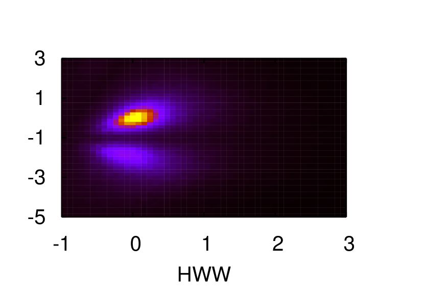
Figure 5: The result of the profile likelihood is shown for the Htt versus the HWW couplings on the (left) without allowing additional contributions to effective couplings and on the (right) allowing additional contributions to effective couplings.

Another difficult scenario at the LHC would be that only a light boson with a mass of about 120 GeV is discovered at the LHC but no (other) new particles. The expected measurement channels and their experimental and theoretical errors are shown in Table 3. While an ILC is capable of a model independent search for the Higgs boson, at the LHC the search and measurement is restricted to well defined final states. Studying the precision of the determination of the Higgs couplings could shed light on new physics.

The study presented here [19] uses essentially the same MonteCarloData as [18] with two important differences: In agrement with more recent experimental studies by ATLAS and CMS [20, 21], the ttH$\rightarrow$bb signal is reduced by 50%. On the other hand the new theoretical analysis of the ZH($\rightarrow$bb) (subjet analysis) [22] is used, confirmed by ATLAS within 10% [23].

The theoretical errors on the production cross section are between 7% and 13%. The errors on the branching ratio calculations are between 1% and 4% (c quarks). The experimental errors have a statistical uncorrelated component and a several sources of systematic error which are highly correlated among measurements. Determining the Higgs couplings from this system is therefore similar to the determination of supersymmetric parameters, i.e., the same techniques can be used to extract the couplings. The additional difficulty to be mastered as some of the channels are in the Poisson regime is the convolution of the flat, Gaussian and Poisson errors.

The parameters are defined in the following way for tree level couplings:

$$g_{jjH}\longrightarrow g_{jjH}^{\mathrm{SM}}\;\left(1+\Delta_{jjH}\right)$$ (1)

as deviations from the Standard Model value. For the loop induced couplings such as the $\gamma\gamma$H and ggH couplings, the definition is as follows

$$g_{jjH}\longrightarrow g_{jjH}^{\mathrm{SM}}\;\left(1+\Delta_{jjH}^{\mathrm{SM}}+\Delta_{jjH}\right)$$ (2)

The additional term $\Delta_{jjH}^{\mathrm{SM}}$ is the modification of the jjH effective coupling induced by a deviation of the tree level couplings of the particles in the loop.

As in the supersymmetric case, first a full dimensional likelihood map is calculated from which the Bayesian and frequentist projections are possible. In the Higgs analysis however no true secondary minima exist and the noise effects of the Bayesian integration are large, essentially washing out the signal. Therefore only the frequentist projection is pursued.

Two main observations can be made after the projections to two dimensions: there is a general positive correlation among all couplings with the exception of the bbH coupling. This is due to the fact that for a Higgs boson mass of 120 GeV the total width is dominated by the decay to b-quarks (approximately 90%). The total width enters in the denominator of every observable, whereas the individual partial widths, proportional to the couplings (squared) enter in the numerator.

The second observation, as shown in Figure 5 (left), is that as long as no additional contributions in the loop induced couplings are allowed ($\Delta_{jjH}$ fixed to 0), a preference for the correct sign of the ttH coupling with respect to the WWH coupling is observed. This is due to the Higgs decay channel to photons. Allowing genuine anomalous couplings in the loop induced couplings destroys this distinction completely as the additional parameter allows for the compensation of the sign preference without a penality to be paid in the $\chi^{2}$ value.

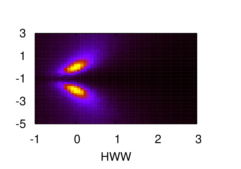
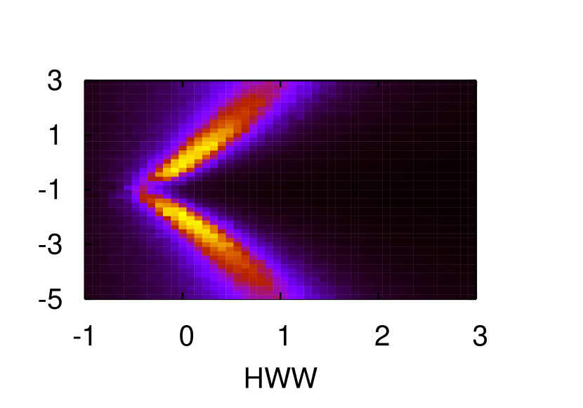
Figure 6: The impact of the subjet analysis on the Higgs boson coupling determination is shown. On the (left) the full sensitivity is used, on the (right) the channel is removed completely.

It is also illustrative to remember what the LHC cannot do in addition to what it can do. All observables are have the structure (simplified) of cross section times branching ratio. Expressed in partial widths we have $\Gamma_{iiH}\Gamma_{jjH}/\Gamma_{tot}$. As partial widths are proportional to the square of the couplings, the structure becomes $g^{2}g^{2}/\Gamma_{tot}$. Thus if a coupling not measured at the LHC, e.g. Hcc is much larger than expected, the total width will increase, but the coupling determination would show deviations from the Standard Model, i.e., couplings smaller than expected. A simultaneous determination of the individual couplings and the total width is not possible as no model independent channel is available. Thus the LHC can measure absolute couplings only under the assumption that all non–measured couplings are equal to their Standard Model prediction.

With this caveat in mind, assuming an integrated luminosity of 30 fb^-1, the Higgs boson couplings can be determined with a precision of 30% (WWH) to 50% (ttH). As before toy experiments were used to obtain these results. The precision is somewhat affected [19] by whether effective couplings are allowed to vary or not. The effect is of the order of up to 20% (relative). If the ratios of couplings are analysed instead of the couplings and the WWH coupling is used as reference, the precision is of the order of 30%. While part of the theoretical and experimental error cancel and therefore one could expect some improvement, with an integrated luminosity of 30 fb^-1 the statistical error is still dominant. The conclusions could therefore change as more data will become available.

In Figure 6 (left) the (bbH,WWH) coupling plane is shown using the full sensitivity of the analysis. In the same Figure (right) the impact of removing the analysis completely is shown. The spread of the central region is much larger. The subjet analysis is essential for the Higgs coupling determination at the LHC because of the importance of the bbH coupling for low Higgs boson masses.

Once the Higgs couplings are determined one can ask whether the precision is sufficient to exclude new physics. The task looks daunting given the precision of the individual couplings. However not only the individual couplings are important but also their correlations. The loglikelihood is used as an estimator take all correlations into account.

In the gluophobic Higgs [24] model the stop quark and top quark contributions cancel to reduce the ggH coupling to 24% of the Standard Model value, i.e. the cross section for gluon fusion processes is reduced by a factor 25. In this case at 90% C.L. 46% of the toy experiments are not described by the Standard Model.

In a second scenario the parameter set SPS1a was moved out of the decoupling region by modifying the mass of the CP–odd Higgs boson A, the top tri–linear coupling and $\tan\beta$. Some of the channels are enhanced, others are reduced by almost 40%. At 90% C.L. 77% of the toy experiments are not described by the Standard Model.

6 CONCLUSIONS

If vintage supersymmetry, as hinted by the electroweak fits, is found at the LHC, a large number of measurements will be available which can be translated into the fundamental parameters of mSUGRA and even the MSSM. To unambiguously determine the parameter set and measure grand unification of the breaking parameters however the ILC will be necessary. The LHC is prepared to determine the fundamental parameters in difficult scenarios, e.g., if only a Higgs boson is discovered at the LHC. A determination of the Higgs couplings can shed light on new physics.

The extraction of the fundamental parameters of any theoretical model is a formidable task which requires a close collaboration of experimentalists and theorists to develop the sophisticated analyses to determine the fundamental parameters at the LHC (and beyond at the ILC) whatever nature has in store.

References

- [1] B. C. Allanach et al., in Proc. of the APS/DPF/DPB Summer Study on the Future of Particle Physics (Snowmass 2001) ed. N. Graf, Eur. Phys. J. C 25 (2002) 113 [arXiv:hep-ph/0202233].
- [2] G. Weiglein et al. [LHC/LC Study Group], Phys. Rept. 426 (2006) 47 [arXiv:hep-ph/0410364].
- [3] B. C. Allanach, Eur. Phys. J. C 59, 427 (2009) [arXiv:0805.2088 [hep-ph]].
- [4] G. A. Blair, W. Porod and P. M. Zerwas, Eur. Phys. J. C 27 (2003) 263 [arXiv:hep-ph/0210058].
- [5] P. Bechtle, K. Desch, W. Porod and P. Wienemann, Eur. Phys. J. C 46, 533 (2006) [arXiv:hep-ph/0511006].
- [6] R. Lafaye, T. Plehn and D. Zerwas, arXiv:hep-ph/0404282.
- [7] R. Lafaye, T. Plehn, M. Rauch and D. Zerwas, Eur. Phys. J. C 54 (2008) 617 [arXiv:0709.3985 [hep-ph]].
- [8] J. Alcaraz et al. [LEP Collaborations and ALEPH Collaboration and DELPHI Collaboration an], arXiv:0712.0929 [hep-ex].
- [9] E. W. Varnes [CDF Collaboration and D0 Collaboration], Int. J. Mod. Phys. A 23, 4421 (2008) [arXiv:0810.3652 [hep-ex]].
- [10] O. Buchmueller et al., JHEP 0809 (2008) 117 [arXiv:0808.4128 [hep-ph]].
- [11] S. S. AbdusSalam, B. C. Allanach, F. Quevedo, F. Feroz and M. Hobson, arXiv:0904.2548 [hep-ph].
- [12] A. Hocker, H. Lacker, S. Laplace and F. Le Diberder, Eur. Phys. J. C 21 (2001) 225 [arXiv:hep-ph/0104062].
- [13] J. A. Aguilar-Saavedra et al., Eur. Phys. J. C 46 (2006) 43 [arXiv:hep-ph/0511344].
- [14] E. A. Baltz, M. Battaglia, M. E. Peskin and T. Wizansky, Phys. Rev. D 74 (2006) 103521 [arXiv:hep-ph/0602187].
- [15] G. F. Giudice and A. Romanino, Nucl. Phys. B 699 (2004) 65 [Erratum-ibid. B 706 (2005) 65] [arXiv:hep-ph/0406088].
- [16] W. Kilian, T. Plehn, P. Richardson and E. Schmidt, Eur. Phys. J. C 39 (2005) 229 [arXiv:hep-ph/0408088].
- [17] N. Bernal, A. Djouadi and P. Slavich, JHEP 0707 (2007) 016 [arXiv:0705.1496 [hep-ph]].
- [18] M. Duhrssen, S. Heinemeyer, H. Logan, D. Rainwater, G. Weiglein and D. Zeppenfeld, Phys. Rev. D 70 (2004) 113009 [arXiv:hep-ph/0406323].
- [19] R. Lafaye, T. Plehn, M. Rauch, D. Zerwas and M. Duhrssen, JHEP 0908 (2009) 009 [arXiv:0904.3866 [hep-ph]].
- [20] G. L. Bayatian et al. [CMS Collaboration], J. Phys. G 34 (2007) 995.
- [21] G. Aad et al. [The ATLAS Collaboration], arXiv:0901.0512 [Unknown].
- [22] J. M. Butterworth, A. R. Davison, M. Rubin and G. P. Salam, Phys. Rev. Lett. 100 (2008) 242001 [arXiv:0802.2470 [hep-ph]].
- [23] ATLAS Collaboration, ATL-PHYS-PUB-2009-088.
- [24] A. Djouadi, Phys. Lett. B 435 (1998) 101 [arXiv:hep-ph/9806315].