Kowalevski’s analysis of the swinging Atwood’s machine.

Abstract

We study the Kowalevski expansions near singularities of the swinging Atwood’s machine. We show that there is a infinite number of mass ratios $M/m$ where such expansions exist with the maximal number of arbitrary constants. These expansions are of the so–called weak Painlevé type. However, in view of these expansions, it is not possible to distinguish between integrable and non integrable cases.

1 Introduction

The swinging Atwood’s machine is a variable length pendulum of mass $m$ on the left, and a non swinging mass $M$ on the right, tied together by a string, in a constant gravitational field, see Figure (1). The coupling of the two masses is expressed by the fact that the length of the string is fixed:

$$\sqrt{x^{2}+y^{2}}+|z|=L,\quad\Longrightarrow x^{2}+y^{2}=(|z|-L)^{2}$$

Up to a choice of origin for z, one can assume $L=0$, so the constraint is the cone $z^{2}=x^{2}+y^{2}$. To describe the dynamics we choose to work with constrained variables and write a Lagrangian

$${\cal L}={m\over 2}(\dot{x}^{2}+\dot{y}^{2})+{M\over 2}\dot{z}^{2}-g(my+Mz)+{\lambda\over 2}(x^{2}+y^{2}-z^{2})$$

where $\lambda$, a Lagrange multiplier (of dimension $MT^{-2}$), has been introduced, whose equation of motion enforces the constraint. The equations of motion read :

$$m\ddot{x} = \lambda x$$ (1)

$$m\ddot{y} = -mg+\lambda y$$ (2)

$$M\ddot{z} = -Mg-\lambda z$$ (3)

$$0 = x^{2}+y^{2}-z^{2}$$ (4)

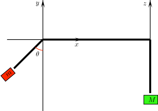
Figure 1: Swinging Atwood’s machine.

From these equations one can express $\lambda$ in terms of positions and velocities:

$$\lambda={x\ddot{x}+y\ddot{y}-z\ddot{z}+g(y-z)\over{1\over m}(x^{2}+y^{2})+{1\over M}z^{2}}={mM\over M+m}{\dot{z}^{2}-\dot{x}^{2}-\dot{y}^{2}+g(y-z)\over z^{2}}$$ (5)

Alternatively, rescaling

$$x\to{1\over\sqrt{m}}x,\quad y\to{1\over\sqrt{m}}y,\quad z\to{1\over\sqrt{M}}z$$

we can view the system as a unit mass particle moving on a cone

$$z^{2}={M\over m}(x^{2}+y^{2})$$

subjected to a constant field force

$$\pmatrix{f_{x}\cr f_{y}\cr fz}=\pmatrix{0\cr-g\sqrt{m}\cr-g\sqrt{M}}$$

The slope of the force in the $(y,z)$ plane coincides with the angle of the cone.

The swinging Atwood’s machine has been studied in great detail by N. Tufillaro and his coworkers, see [1–7]. They have first studied numerically the equations of motion and shown that for most values of the mass ratio $M/m$ the motion appears to be chaotic, however for some values, like 3, 15, etc. the motion seems less chaotic and could perhaps be integrable. In a further study, Tufillaro [4] showed that the system is indeed integrable for $M/m=3$ by exhibiting a change of coordinates, somewhat related to parabolic coordinates, in which separation of variables occurs. He was then able to solve the equations of motion in terms of elliptic functions, which is quite peculiar since in general integrable systems with two degrees of freedom can be solved only in terms of hyperelliptic functions, such as for the Kowalevski top [8]. He also obtained the second conserved quantity which ensures integrability. In the same paper, he conjectured that the system is integrable for $M/m=15,\cdots,4n^{2}-1$, with $n$ integer.

However, later on, Casasayas, Nunes and Tufillaro proved [6] that the system can be integrable for discrete values of the ratio $M/m$ only in the interval $]1,3]$, using non integrability theorems developed by Yoshida [9] and Ziglin. The essence of the Yoshida–Ziglin argument is to study the monodromy developed by Jacobi variations around an exact solution, when the time variable describes a loop in the complex plane. The monodromy must preserve conserved quantities, but this is impossible in general if the monodromy group is not abelian. In the case at hand one can compute monodromies from hypergeometric equations and conclude. We have also been informed by private communication of J.P. Ramis, that he and his coworkers have proven that the swinging Atwood’s machine is never integrable except for $M/m=3$, using methods from differential Galois theory.

The aim of our paper is to work out the Kowalevski analysis for this model. Let us recall the idea of the Kowalevski method. If a dynamical system is algebraically integrable one can expect to obtain expressions for the dynamical variables in terms of quotients of theta functions defined on the Jacobian of some algebraic curve of genus g, where g=2 for a system with 2 degrees of freedom. Only quotients may appear because theta functions have monodromy on the Jacobian torus, which needs to cancel. Hence denominators which can vanish for any given initial conditions and for some finite value, in general complex, of time will appear in the solution. Hence the equations of motion must admit Laurent solutions –that is divergent for some value of time, with as many parameters as there are initial conditions. S. Kowalevski first noted [8], that this imposes strong constraints on these equations, from which she was able to deduce the celebrated Kowalevski case of the top equation.

Looking for Laurent solutions to the swinging Atwood’s machine equations of motion in the integrable case $M/m=3$ we first noted that there are none, but there exists so-called weak Painlevé solutions, that is Laurent developments not in the time variable $t$ but in some radical $t^{1/k}$, generally called Puiseux expansions.

It had already been discovered by A. Ramani and coworkers [10] that some integrable systems require weakening the Kowalevski–Painlevé analysis to obtain expansions at infinity of dynamical variables. This may be explained in general, and is certainly the case for our example, by the fact that there is a “better” variable which has true Laurent expansions and time itself can be expressed in terms of this variable through an algebraic equation which happens to produce the given radicals. Moreover Ramani et al. advocated the idea that the existence of weak Painlevé solutions is a criterion of integrability, like in the Kowalevski’s case.

For our model of the swinging Atwood’s machine, we find that there are weak Painlevé solutions not only when $M/m=15$ but for a whole host of other values of the mass ratio, all of them corresponding to obviously non integrable cases. Hence this model provides a large number of counterexamples to the above idea. We then study in detail the solutions around infinity which can be extracted from these Kowalevski developments. Using Padé approximants we are able to extend these solutions beyond the first new singularity and observe how the new singularities obey Kowalevski exponents.

We also comment on the Poisson structure of the model, which is interesting due to the constraints between the dynamical variables, and the Poisson brackets of the variables appearing in the Laurent series, which happens to be of a nice canonical form. We notice that this illustrates the fact that it is the global character of the conserved quantities that is of importance in defining an integrable system.

One of us (M.T.) is happy to acknowledge useful conversations with J.P. Ramis and J. Sauloy from Toulouse University, about their work on differential Galois theory applied to the swinging Atwood’s machine. Finally we are happy to thank the Maxima team for their software, with which we have performed the computations in this paper.

2 Hamiltonian setup.

The description we have given of the swinging Atwood’s machine is a constrained system in the Lagrange formulation, so that the equations of motion take a nice algebraic form.

In the articles [1–7] polar coordinates are used, so the constraint is “solved” but the price to pay is the use of trigonometric functions. Using polar coordinates $x=r\sin\theta$, $y=-r\cos\theta$ the Hamiltonian reads:

$$H={1\over 2(m+M)}p_{r}^{2}+{1\over 2mr^{2}}p_{\theta}^{2}+gr(M-m\cos\theta)$$ (6)

where $p_{r}=(m+M)\dot{r}$ and $p_{\theta}=mr^{2}\dot{\theta}$.

We now give a Hamiltonian description of this system, using as dynamical variables the three coordinates $x,y,z$ and the three momenta $p_{x},p_{y},p_{z}$ with canonical Poisson brackets. The constraint

$$C_{1}\equiv z^{2}-x^{2}-y^{2}=0$$ (7)

generates the flow:

$$\{C_{1},p_{x}\}=-2x,\quad\{C_{1},p_{y}\}=-2y,\quad\{C_{1},p_{z}\}=2z$$ (8)

which is also generated by the one parameter group acting on phase space by: $(x,y,z)\to(x,y,z),\quad(p_{x},p_{y},p_{z})\to(p_{x}-\mu x,p_{y}-\mu y,p_{z}+\mu z)$ where $\mu$ is the group parameter.

We want to describe the dynamics of our model as a Hamiltonian system obtained by reduction of an invariant system under this group action [11]. In order to do that, consider the functions:

$$A_{x} = zp_{y}+yp_{z}$$

$$A_{y} = zp_{x}+xp_{z}$$

$$A_{z} = xp_{y}-yp_{x}$$

These functions Poisson commute with the constraint $C_{1}$ hence are invariant under the group action. They are not independent however, since they are related by:

$$yA_{y}-xA_{x}+zA_{z}=0$$ (9)

It is easy to check the Poisson brackets:

$$\{A_{x},A_{y}\}=-A_{z},\quad\{A_{x},A_{z}\}=-A_{y},\quad\{A_{y},A_{z}\}=A_{x}$$

$$\{A_{x},x\}=0,\quad\{A_{x},y\}=z,\quad\{A_{x},z\}=y$$

$$\{A_{y},x\}=z,\quad\{A_{y},y\}=0,\quad\{A_{y},z\}=x$$

$$\{A_{z},x\}=-y,\quad\{A_{z},y\}=x,\quad\{A_{z},z\}=0$$

Let us consider the invariant Hamiltonian:

$$H={1\over 2(m+M)z^{2}}\left[A_{x}^{2}+A_{y}^{2}+{M\over m}A_{z}^{2}\right]+Mgz+mgy$$ (10)

To check that $H$ generates the equations of motion on the reduced system, we compute:

$$\dot{x}=\{H,x\} = {1\over m+M}{1\over z^{2}}\left(zA_{y}-{M\over m}yA_{z}\right)$$ (11)

$$\dot{y}=\{H,y\} = {1\over m+M}{1\over z^{2}}\left(zA_{x}+{M\over m}xA_{z}\right)$$ (12)

$$\dot{z}=\{H,z\} = {1\over m+M}{1\over z^{2}}\left(xA_{y}+yA_{x}\right)$$ (13)

The right hand sides of these equations are linear in the momenta $p_{x}$, $p_{y}$, $p_{z}$, however we cannot invert the system uniquely in order to express the momenta in terms of the velocities. This is because, due to the symmetry ($\{H,C_{1}\}=0$) we have $x\dot{x}+y\dot{y}=z\dot{z}$ so the equations are not independent. The solution is:

$$p_{x} = m\dot{x}+\mu x$$ (14)

$$p_{y} = m\dot{y}+\mu y$$ (15)

$$p_{z} = M\dot{z}-\mu z$$ (16)

where $\mu$ is arbitrary. Similarly we compute $\ddot{x}=\{H,\dot{x}\}$, etc… where $\dot{x}$, etc… are the right hand sides of the above equations. Performing this calculation and using the constraint $C_{1}$ and eq.(9), we obtain the Lagrangian equation of motion (1–3), with $\lambda$ given by:

$$\lambda={mM\over m+M}{1\over z^{2}}\left[g(y-z)-{1\over m^{2}z^{2}}A_{z}^{2}\right]$$

This coincides with eq.(5), as can be cheked using again eqs.(14–16) and the constraint $C_{1}$, to express $A_{z}$ in terms of $\dot{x}$, $\dot{y}$, $\dot{z}$.

Finally we express the energy in terms of velocities still using the constraints. We find:

$$E={m\over 2}(\dot{x}^{2}+\dot{y}^{2})+{M\over 2}\dot{z}^{2}+g(my+Mz)$$ (17)

which agrees with what we expect from the Lagrangian formulation.

3 The integrable case.

In order to understand what sort of Laurent expansions appears in the model it is useful to first consider the case $M/m=3$ which has been integrated by Tufillaro [4]. Let us recall some of his results. He discovered that using polar coordinates $(r,\theta)$ such that $x=r\sin\theta$, $y=-r\cos\theta$ and $r=z$, and setting:

$$\xi^{2}=z[1+\sin(\theta/2)],\quad\eta^{2}=z[1-\sin(\theta/2)]$$

then the Hamilton–Jacobi equation separates in the variables $(\xi,\eta)$. These look like parabolic coordinates, except that the half–angle $\theta/2$ is used. Knowing $\xi$ and $\eta$ one can recover $x$ and $y$ by:

$$x_{\pm}\equiv x\pm iy=\pm{i\over 2}{(\xi\mp i\eta)^{3}\over(\xi\pm i\eta)},\quad z={1\over 2}(\xi^{2}+\eta^{2})$$ (18)

In fact, just for $M=3m$, two terms involving couplings between $\xi$ and $\eta$ disappear, and one gets, with momenta $p_{\xi}=4\dot{\xi}(\xi^{2}+\eta^{2})$ etc. the expression of the Hamiltonian, in which we have set $m=1$:

$$H=[(p_{\xi}^{2}+p_{\eta}^{2})/8+2g(\xi^{4}+\eta^{4})]/(\xi^{2}+\eta^{2})$$

Then it is clear that in this case the action $S$ separates as a sum $S_{\xi}(\xi)+S_{\eta}(\eta)$ where $S_{\xi}$ and $S_{\eta}$ obey different elliptic equations (corresponding to different elliptic moduli):

$$(\partial_{\xi}S_{\xi})^{2} = -16g\xi^{4}+8E\xi^{2}+I\equiv P_{+}(\xi)$$ (19)

$$(\partial_{\eta}S_{\eta})^{2} = -16g\eta^{4}+8E\eta^{2}-I\equiv P_{-}(\eta)$$ (20)

where I is the separation constant. It can be expressed in terms of dynamical variables by substracting the above two equations multiplied resp. by $\eta^{2}$ and $\xi^{2}$, which eliminates $E$. Moreover we replace:

$$\partial_{\xi}S=p_{\xi}=4\dot{\xi}(\xi^{2}+\eta^{2}),\quad\partial_{\eta}S=p_{\eta}=4\dot{\eta}(\xi^{2}+\eta^{2})$$ (21)

We get:

$$I/16=(\xi^{2}+\eta^{2})(\eta^{2}\dot{\xi}^{2}-\xi^{2}\dot{\eta}^{2})+g\xi^{2}\eta^{2}(\xi^{2}-\eta^{2})/(\xi^{2}+\eta^{2})$$

Returning to polar coordinates the integral of motion takes the form:

$$I/16=r^{2}\dot{\theta}\big{[}\dot{r}\cos(\theta/2)-{r\dot{\theta}\over 2}\sin(\theta/2)\big{]}+gr^{2}\sin(\theta/2)\cos^{2}(\theta/2)$$

We want to see if the equations of motion admit a solution which diverges at finite time, and in that case what is the behavior of the Laurent expansion.

The general solution of the Hamilton–Jacobi equation is:

$$S=-Et+\int^{\xi}\sqrt{P_{+}(\xi)}\,d\xi+\int^{\eta}\sqrt{P_{-}(\eta)}\,d\eta$$

According to the general theory we get the solution of the equations of motion by writing $\partial_{E}S=c_{E}$ and $\partial_{I}S=c_{I}$ for two constants $c_{E}$ and $c_{I}$. For $c_{I}\neq 0$ we get:

$$t+c_{E} = \int^{\xi}{4\xi^{2}\over\sqrt{P_{+}(\xi)}}d\xi+\int^{\eta}{4\eta^{2}\over\sqrt{P_{-}(\eta)}}d\eta$$ (22)

$$c_{I} = {1\over 2}\int^{\xi}{1\over\sqrt{P_{+}(\xi)}}d\xi-{1\over 2}\int^{\eta}{1\over\sqrt{P_{-}(\eta)}}d\eta$$ (23)

For $I=0$, the elliptic integrals degenerate to trigonometric ones. We get:

$$t+c_{E}=-{1\over 2\omega}\left(\sqrt{1-\alpha\xi^{2}}+\sqrt{1-\alpha\eta^{2}}\right),~{}\alpha=2g/E,~{}\omega=g/\sqrt{2E}$$ (24)

$${1-\sqrt{1-\alpha\xi^{2}}\over 1+\sqrt{1-\alpha\xi^{2}}}=K^{2}{1-\sqrt{1-\alpha\eta^{2}}\over 1+\sqrt{1-\alpha\eta^{2}}},\quad K^{2}=e^{c_{I}}$$ (25)

so that setting $\xi=\sin(\phi_{\xi})/\sqrt{\alpha},\;\eta=\sin(\phi_{\eta})/\sqrt{\alpha}$ the second equality reads:

$$\tan(\phi_{\xi}/2)=K\tan(\phi_{\eta}/2)$$

Using the variable $s=\tan(\phi_{\xi}/2)$, $\xi$ and $\eta$ can be expressed rationally:

$$\xi={1\over\sqrt{\alpha}}{2s\over 1+s^{2}},\quad\eta={1\over\sqrt{\alpha}}{2Ks\over K^{2}+s^{2}}$$

Finally, one gets the time variation of $S\equiv s^{2}$ by using eq.(24) which implies:

$$\omega dt=dS\left[{1\over(1+S)^{2}}+{K^{2}\over(K^{2}+S)^{2}}\right]=-{8iK\over K^{2}-1}{U\,dU\over(U^{2}-1)^{2}}$$

where we have parametrized $S$ as:

$$S=iK\,{(K+i)U+(K-i)\over(K-i)U-(K+i)}$$

The variable $U$ has been defined to send the poles $S=-K^{2}$ and $S=-1$ to $U=\pm 1$. One gets the two parameters solution (parameters $K$ and $E$) up to an origin for time, which we fix by requiring that $t=0$ for $U=0$:

$$U^{2}={t\over t-t_{\infty}}~{}{\rm or}~{}U^{2}-1={t_{\infty}\over t-t_{\infty}}\Longrightarrow t=-t_{\infty}{U^{2}\over 1-U^{2}},\quad t_{\infty}={1\over\omega}{4iK\over K^{2}-1}$$

We shall soon see that $t=t_{\infty}$ is a second singularity of the dynamical variables, that we can express explicitly. For ease of comparison with the following, we present $x_{\pm}(t)=x(t)\pm iy(t)$:

$$x_{+} = -{2Kg\over\omega^{2}}\;{\left[(K-i)U-K-i\right]\,\left[(K+i)U+K-i\right]\over{(K^{2}-1)^{2}(U^{2}-1)^{2}}}\,{1\over U}$$

$$x_{-} = {2Kg\over\omega^{2}}\;{\left[(K-i)U-K-i\right]\,\left[(K+i)U+K-i\right]\over{(K^{2}-1)^{2}(U^{2}-1)^{2}}}\,U^{3}$$

$$z = i{2Kg\over\omega^{2}}\;{\left[(K-i)U-K-i\right]\,\left[(K+i)U+K-i\right]\over{(K^{2}-1)^{2}(U^{2}-1)^{2}}}\,U$$

$$\lambda = -{3\omega^{2}\over 64K^{2}}{(K^{2}-1)^{2}(K^{2}+1)(U^{2}-1)^{5}\over\left[(K-i)U-K-i\right]\,\left[(K+i)U+K-i\right]U^{4}}$$

In terms of the $t$ variable, we get the simpler expressions:

$$x_{+}(t) = -{2Kg\over\omega^{2}(K^{2}-1)^{2}}\left[(K^{2}+1){\left({t-t_{\infty}\over t_{\infty}}\right)^{3/2}}\left({t_{\infty}\over t}\right)^{1/2}-4iK\left({t-t_{\infty}\over t_{\infty}}\right)^{2}\right]$$

$$x_{-}(t) = {2Kg\over\omega^{2}(K^{2}-1)^{2}}\left[(K^{2}+1)\left({t\over t_{\infty}}\right)^{3/2}\left({t_{\infty}\over t-t_{\infty}}\right)^{1/2}-4iK\left({t\over t_{\infty}}\right)^{2}\right]$$

We see that $x_{+}$ behaves as $t^{-{1\over 2}}$ and $x_{-}$ behaves as $t^{3\over 2}$ when $t\to 0$. If we expand around $t=0$ we get Puiseux expansions in $t^{1\over 2}$. These expansions depend on three parameters, $K$ and $E$ plus the origin of time $t_{0}$. This is because we are analyzing the trigonometric solution which fixes one of the constants to $I=0$. We shall see later on that it can be generalized to a four parameter expansion in the elliptic case. The energy parameter appears factorized in front of $x_{+}$ and $x_{-}$ in the form of $g/\omega^{2}=2E/g$.

Around $t_{\infty}$, we see that $x_{+}$ behaves as $(t-t_{\infty})^{3\over 2}$ and $x_{-}$ behaves as $(t-t_{\infty})^{-{1\over 2}}$ which is symmetrical with the behaviour at $t=0$. This is compatible with the fact that the equations of motion admit a symmetry $(x_{+}(t),x_{-}(t))\leftrightarrow(-x_{-}(t),-x_{+}(t))$.

Remark that $x_{\pm}(t)$ are defined on the two sheeted covering of the Riemann sphere with two branch points at $t=0$ and $t=t_{\infty}$. The variable $U$ that we have introduced is in fact a uniformizing variable for this covering, so that $x_{\pm}(t)$ are rational functions of $U$. Moreover $U\leftrightarrow-1/U$ corresponds to $t\leftrightarrow(t_{\infty}-t)$ and exchanges $x_{+}$ and $-x_{-}$. The extra minus sign means that we have to change the determination of the square root in the $t$ variable. The $U$ variable makes this completely unambiguous:

$$x_{+}\left(-{1\over U}\right)=-x_{-}(U),\quad z\left(-{1\over U}\right)=z(U),\quad\lambda\left(-{1\over U}\right)=\lambda(U)$$

We emphasize that, although the system is integrable, the solutions diverge with square root singularities at finite times $t=0$, and $t=t_{\infty}$.

We now return to the elliptic case. Let us define the variables $X=\xi^{2}-E/(6g)$ and $Y=\eta^{2}-E/(6g)$. The equations (22,23) become:

$$t+c_{E} = {1\over 4i\sqrt{g}}\int^{X}{(X+E/(6g))dX\over\sqrt{P_{+}(X)}}+{1\over 4i\sqrt{g}}\int^{Y}{(Y+E/(6g))dY\over\sqrt{P_{-}(Y)}}$$

$$c_{I} = {1\over 4i\sqrt{g}}\int^{X}{dX\over\sqrt{P_{+}(X)}}-{1\over 4i\sqrt{g}}\int^{Y}{dY\over\sqrt{P_{-}(Y)}}$$

where now:

$$P_{\pm}(X)=4X^{3}-g_{2}(\pm I)X-g_{3}(\pm I)$$

$$g_{2}(I)={1\over 3g^{2}}\left(E^{2}+{3\over 4}gI\right),\quad g_{3}(I)={E\over 27g^{3}}\left(E^{2}+{9\over 8}gI\right)$$

Introducing the Weierstrass functions

$$X=\wp_{1}(Z_{1})\equiv\wp(Z_{1},g_{2}(I),g_{3}(I)),\quad Y=\wp_{2}(Z_{2})\equiv\wp(Z_{2},g_{2}(-I),g_{3}(-I))$$

the above integrals reduce to:

$$t+c_{E} = {1\over 4i\sqrt{g}}\left[{E\over 6g}(Z_{1}+Z_{2})-\zeta_{1}(Z_{1})-\zeta_{2}(Z_{2})\right]$$ (28)

$$c_{I} = {1\over 4i\sqrt{g}}\left[Z_{1}-Z_{2}\right]$$ (29)

where $\zeta$ is the Weierstrass zeta function, $\zeta^{\prime}=-\wp$. The $\wp$ function has two periods 2$\omega_{j}$, $j=1,2$, so that $\wp(z+2\omega_{j})=\wp(z)$, but the zeta function is quasi periodic, $\zeta(z+2\omega_{j})=\zeta(z)+2\eta_{j}$. Here we have two set of periods $\omega_{j}$ and $\eta_{j}$ according to the function $\wp_{1}$ or $\wp_{2}$, which are in fact functions $\omega_{j}(\pm I)$ and $\eta_{j}(\pm I)$.

Note that $x_{\pm}(t)$ have poles and zeroes when $\xi\pm i\eta$ vanish, that is when $\xi^{2}+\eta^{2}=X+Y+E/(3g)=0$. Hence we have to solve:

$$E/(3g)+\wp_{1}(Z_{1})+\wp_{2}(Z_{2})=0$$ (30)

$$Z_{1}-Z_{2}-4i\sqrt{g}c_{I}=0$$ (31)

But differentiating eqs.(28,29) we find $\delta Z_{2}=\delta Z_{1}$ and

$$\delta t={1\over 4i\sqrt{g}}\left({E\over 3g}+\wp_{1}(Z_{1})+\wp_{2}(Z_{2})\right)\delta Z_{1}+{1\over 8i\sqrt{g}}\left(\wp_{1}^{\prime}(Z_{1})+\wp_{2}^{\prime}(Z_{2})\right)(\delta Z_{1})^{2}+\cdots$$

The first term vanishes when $\xi^{2}+\eta^{2}=0$ hence around such a zero $\delta Z_{1}\simeq\sqrt{\delta t}$. As a consequence, in view of eq.(18), $x_{\pm}(t)$ behaves as either $\delta t^{-1/2}$ or $\delta t^{3/2}$ at such a point, according to the vanishing of $\xi+i\eta$ or $\xi-i\eta$. Note this is similar to the trigonometric case.

However finding the pattern of these singularities is messy, because in the equations (30,31) we have two incommensurate lattices of periods for the two Weierstrass functions. However we can easily see that there is an infinite number of singularities. This is because since the two lattices are incommensurate, for any large $R$ and small $\epsilon$, one can choose $V$ in the first lattice and $W$ in the second, such that $|V-W|<\epsilon$ and $|V|,~{}|W|>R$. Starting from a solution $Z_{1}$, $Z_{2}$ of our equations, we set $Z^{\prime}_{1}=Z_{1}+V$ and $Z^{\prime}_{2}=Z_{2}+W$, which still obey eq.(30). However eq.(31) is violated at order $\epsilon$. Choose $Z^{\prime\prime}_{1}=Z^{\prime}_{1},~{}Z^{\prime\prime}_{2}=Z^{\prime\prime}_{1}-4i\sqrt{g}c_{I}$ and plug this in eq.(30). It then gets of order $\epsilon$ but this is an equation for the variable $Z_{1}$ which has, by complex analyticity, an exact solution close to this approximate solution. Taking larger and larger values for $R$ one gets an infinite number of solutions. Around each of these solutions we have Puiseux expansions in the variable $\delta t^{1/2}$.

4 Kowalevski analysis.

If the swinging Atwood’s machine is an algebraically integrable system the dynamical variables can be expressed algebraically in terms of a linear motion on some Abelian variety, in particular all variables and time can be complexified at will. We may expect that, for general initial conditions, the dynamical variables will blow out for some (in general complex) value $t_{0}$ of the time $t$. Around this value the dynamical variables should have Laurent behavior, hence one expects to find Laurent solutions depending on $N$ parameters (initial conditions) if the phase space is of dimension $N$. In practice one searchs for Laurent expansions at $t=0$ (one fixes $t_{0}=0$) so an admissible Laurent solution should have $N-1$ parameters, that is 3 parameters for the example at hand.

The Puiseux solutions we have found in previous section have the following singularity: $x$ and $y$ blow up but $z\to 0$, hence $x^{2}+y^{2}\to 0$. This means that the singular solutions are such that the mass $m$ goes to the origin but rotating faster and faster. If we expand $x$ and $y$ in negative powers of $t$ there must be large cancellations such that $x^{2}+y^{2}\to 0$. It is much more convenient to factorize $x^{2}+y^{2}$ and have the cancellation between the two factors. Reminding that:

$$x_{\pm}=x\pm iy$$

the equations of motion are

$$m\ddot{x}_{+} = -img+\lambda x_{+}$$

$$m\ddot{x}_{-} = img+\lambda x_{-}$$

$$M\ddot{z} = -Mg-\lambda z$$

$$z^{2} = x_{+}x_{-}$$ (32)

The value of $\lambda$ is a consequence of these equations:

$$\lambda={mM\over M+m}{\dot{z}^{2}-\dot{x}_{+}\dot{x}_{-}+g(y-z)\over z^{2}}$$

where $y=-i(x_{+}-x_{-})/2$. Let us remark that this system of equations is invariant under $(x_{+},x_{-})\to(-x_{-},-x_{+})$, in particular $y$ and $\lambda$ are invariant. The system is also invariant under a similarity transformation:

$$x_{\pm}(t)\to\mu^{2}x_{\pm}(t/\mu),\quad z(t)\to\mu^{2}z(t/\mu),\quad\lambda(t)\to{1\over\mu^{2}}\lambda(t/\mu)$$

We first analyze equations (32) at the leading order. We thus look for solutions of the form:

$$x_{+}=a_{1}t^{p}+\cdots,\quad x_{-}=b_{1}t^{q}+\cdots,$$

so that eq. (32) requires

$$\quad z=c_{1}\;t^{p+q\over 2}+\cdots,\quad c_{1}^{2}=a_{1}b_{1}$$

At lowest order we then have:

$$\lambda={mM\over 4(M+m)}{a_{1}b_{1}(p-q)^{2}t^{p+q-2}+4g(y-z)\over a_{1}b_{1}t^{p+q}}$$ (33)

Clearly equations of motion (32) require that $\lambda$ behave as $1/t^{2}$ for solutions blowing out as powers. At first sight there are two ways in which this can happen: when the first term in the numerator is dominant, or when the second term is dominant. We can always choose $p\leq q$, up to exchange of $x_{+}$ and $x_{-}$, hence $p<0$ since we want to have at least one dynamical variable diverging. On the other hand $z\to 0$ so $q$ is positive, hence $y-z=O(t^{p})$. The first term is dominant when $q<2$, and for $p\neq q$ one has indeed $\lambda\simeq 1/t^{2}$. When $q=2$ both terms are of the same order and for $q>2$ the second term is dominant, so that $\lambda=O(t^{-q})$ which is not allowed. Hence we have basically only two cases to consider, either $p<0,q<2$ in which the integrable case studied above belongs ($p=-1/2,q=3/2$), or the case $-2<p<0,q=2$, which, as we will see, covers more general values of the mass ratio $M/m$.

4.1 Integrable case.

Since $p<0,q<2$ we have $p+q-2<(p,q,{p+q\over 2})$, and we can neglect the term $g(y-z)$ at leading order in the expression of $\lambda$. We find, for $p\neq q$:

$$\lambda={mM(p-q)^{2}\over 4(M+m)}{1\over t^{2}}+\cdots$$

Similarly the equations of motion for $x_{\pm}$ give:

$$p(p-1)={M\over 4(M+m)}(p-q)^{2}=q(q-1)$$ (34)

so that $(p-q)(p+q-1)=0$ hence, since $p\neq q$, $p<q$ and we have $p+q-1=0$. Since by positivity in eq.(34), $p$ and $q$ cannot belong to $[0,1]$ this implies, together with $p>p+q-2=-1$ that:

$$-1<p<0,\quad 1<q<2$$

Using $p+q=1$ the mass ratio takes the form:

$$M=-4mpq=m[(p-q)^{2}-1]=m[(2p-1)^{2}-1]$$

and the mass ratio $M/m$ is thus in the interval $]0,8[$.

The integrable case corresponds to $M=3m$, and falls into this analysis with:

$$p=-{1\over 2},\quad q={3\over 2}$$

These exponents are exactly those we have found in the exact solution of the elliptic integrable case. There are no other values of $p$ in $]-1,0[$ compatible with integer values of the mass ratio $M/m$ which could, according to [4], correspond to seemingly integrable behaviour. We thus consider, in the following, the integrable case $M/m=3$.

As noted above the second conserved quantity is given in polar coordinates for $m=1$, introducing for convenience $H_{2}=I\,\sqrt{2}/8$, by:

$${1\over 2\sqrt{2}}H_{2}=r^{2}\dot{\theta}{d\over dt}{(r\cos(\theta/2))}+{g\over 2}(r\sin\theta)(r\cos(\theta/2))$$

which reads in cartesian coordinates as:

$$H_{2}={1\over\sqrt{z(z-y)}}(x\dot{y}-y\dot{x}){d\over dt}(z^{2}-zy)+gx\sqrt{z(z-y)}$$

Taking the square to eliminate the square roots, we get:

$$H_{2}^{2}={1\over z(z-y)}(x\dot{y}-y\dot{x})^{2}\left({d\over dt}(z^{2}-zy)\right)^{2}+2gx(x\dot{y}-y\dot{x}){d\over dt}(z^{2}-zy)+g^{2}x^{2}(z^{2}-zy)$$

We can setup an expansion in powers of $\sqrt{t}$.

$$x_{+} = t^{-{1\over 2}}(a_{1}+a_{2}t^{{1\over 2}}+\cdots)$$

$$x_{-} = t^{3\over 2}(b_{1}+b_{2}t^{{1\over 2}}+\cdots)$$

$$z = t^{{1\over 2}}(d_{1}+d_{2}t^{{1\over 2}}+\cdots)$$

$$\lambda = t^{-2}(l_{1}+l_{2}t^{1\over 2}+\cdots)$$

We already know that

$$a_{1}b_{1}=d_{1}^{2},\quad l_{1}={3m\over 4}$$

Inserting into the equations of motion, we find the recursive system:

$${\cal K}(s)\cdot\pmatrix{a_{s+1}\cr b_{s+1}\cr d_{s+1}\cr l_{s+1}}=\pmatrix{A_{s+1}\cr B_{s+1}\cr D_{s+1}\cr L_{s+1}}$$

$${\cal K}(s)=\pmatrix{m{(s-1)(s-3)\over 4}-l_{1}&0&0&-a_{1}\cr 0&m{(s+1)(s+3)\over 4}-l_{1}&0&-b_{1}\cr 0&0&M{(s+1)(s-1)\over 4}+l_{1}&d_{1}\cr-b_{1}&-a_{1}&2d_{1}&0}$$

The square matrix in the left hand side is called the Kowalevski matrix, and the vector in the right hand side is given by

$$A_{s+1} = \sum_{j=1}^{s-1}l_{j+1}a_{s-j+1}-img\delta_{s,5}$$

$$B_{s+1} = \sum_{j=1}^{s-1}l_{j+1}b_{s-j+1}+img\delta_{s,1}$$

$$D_{s+1} = -\sum_{j=1}^{s-1}l_{j+1}d_{s-j+1}-Mg\delta_{s,3}$$

$$L_{s+1} = -\sum_{j=1}^{s-1}d_{j+1}d_{s-j+1}+\sum_{j=1}^{s-1}a_{j+1}b_{s-j+1}$$

The determinant of the Kowalevski matrix reads

$$\det({\cal K}(s))=-{m^{2}d_{1}^{2}\over 2}(s+2)s^{2}(s-2)$$

It has a double zero at $s=0$ and a third zero at the integer value $s=2$. Hence potentially three arbitrary constants may appear in the expansion. Indeed the miracle happens at the third level where the equations determining the coefficients $a_{3},b_{3}$ are degenerate, leaving one extra constant $b_{3}=c_{1}$. The rest of the expansion is then completely determined at all orders. We find in particular:

$$x_{+} = {{d_{1}^{2}}\over{b_{1}\,\sqrt{t}}}+{{i\,d_{1}^{2}\,g}\over{2\,b_{1}^{2}}}-{{3\,c_{1}\,d_{1}^{2}\,\sqrt{t}}\over{b_{1}^{2}}}+{{\left(4\,i\,c_{1}\,d_{1}^{2}-7\,b_{1}^{2}\,d_{1}\right)\,g\,t}\over{5\,b_{1}^{3}}}+$$

$$+{{\left(\left(2\,c_{1}\,d_{1}^{2}+i\,b_{1}^{2}\,d_{1}\right)\,g^{2}+12\,b_{1}\,c_{1}^{2}\,d_{1}^{2}\right)\,t^{{{3}\over{2}}}}\over{8\,b_{1}^{4}}}+\cdots$$

$$x_{-} = b_{1}\,t^{{{3}\over{2}}}+{{i\,g\,t^{2}}\over{2}}+c_{1}\,t^{{{5}\over{2}}}-{{\left(2\,i\,c_{1}\,d_{1}-b_{1}^{2}\right)\,g\,t^{3}}\over{5\,b_{1}\,d_{1}}}-$$

$$-{{\left(\left(6\,c_{1}\,d_{1}+3\,i\,b_{1}^{2}\right)\,g^{2}-60\,b_{1}\,c_{1}^{2}\,d_{1}\right)\,t^{{{7}\over{2}}}}\over{40\,b_{1}^{2}\,d_{1}}}+\cdots$$

The existence of such a “miracle” is exactly what S. Kowalevski noted in [8] for her integrable case of the top. For this to happen one needs that the determinant of ${\cal K}(s)$ vanishes for the correct number of integer values of the recursive variable $s$, which allows for a new indeterminate to enter the expansion. Moreover in this case the linear system has to be solvable which is far from guaranteed. The general solution of the equations of motion must admit a power series expansion, which thus must depend on $2N-1$ arbitrary constants for a system of $N$ degrees of freedom. In our case we find a solution depending correctly on three constants, which extends the trigonometric solution described above.

Inserting these expansions into the formula for the energy (17) we obtain:

$$E=-{md_{1}^{2}\over 8b_{1}^{2}}(g^{2}+32c_{1}b_{1})$$

Similarly, the second conserved quantity reads:

$$H_{2}^{2}={2id_{1}^{5}\over b_{1}^{3}}(b_{1}^{2}-2ic_{1}d_{1})^{2}$$

It is interesting to compare these general results to the expansion in the trigonometric case eqs.(LABEL:xplust,LABEL:xmoinst). One finds:

$$b_{1} = e^{-{i\pi\over 4}}{g(K^{2}+1)\over 4\sqrt{\omega}\sqrt{K}\sqrt{K^{2}-1}}$$

$$c_{1} = e^{-{3i\pi\over 4}}{g\sqrt{\omega}\sqrt{K^{2}-1}(K^{2}+1)\over 32K^{3\over 2}}$$

$$d_{1} = e^{-{i\pi\over 4}}{g\sqrt{K}(K^{2}+1)\over\omega^{3\over 2}(K^{2}-1)^{3\over 2}}$$

With these values one checks that $H_{2}=0$ as it should be in the trigonometric case, and that $H$ is indeed equal to $E$.

The dynamical variables $(x,y,z)$ and their time derivatives are expressed in power series of $\sqrt{t}$. These power series have a non vanishing finite radius of convergence (we know this at least in the trigonometric case from the exact solution) and we can check it numerically. To do that we compute the d’Alembert quotient $|a_{n+1}/a_{n}|$ relative to a series $\sum_{n}a_{n}t^{n}$ which tends to the inverse of the radius of convergence of this series when it exists. We present the result of this computation for high order $n$ for the series $x_{+}(t)$, $x_{-}(t)$, $z(t)$, and $\lambda(t)$ in the figure (2).

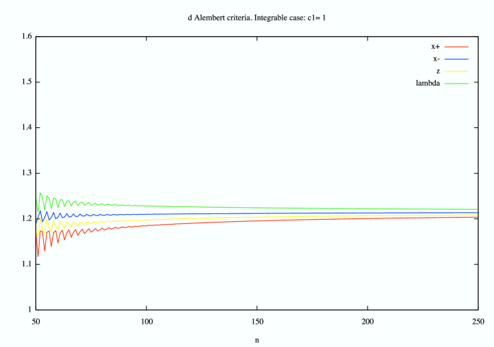
Figure 2: d’Alembert criterium for convergence for p=-1/2, q=3/2.

In this and following similar computations, all values are calculated with absolute precision rational numbers using a formal computation tool. This ensures accuracy of the result.

Since the Kowalevski expansion converges in a disk, the parameters $(b_{1},c_{1},d_{1})$ appearing in these series, and the origin of time $t_{0}$, can be considered as coordinates on an open set of phase space near infinity [12]. The question then arises to compute the Poisson brackets in these coordinates.

To do that, we start from:

$$\{A_{z}(t),x_{\pm}(t)\}=\pm ix_{\pm}(t)$$ (35)

This equation is valid for any time since the time evolution is a canonical transformation. We thus insert into it the series for $x_{\pm}(t)$, where these series are really series in $(t+t_{0})^{1\over 2}$. Similarly

$$A_{z}(t)=i{m\over 2}(x_{+}\dot{x}_{-}-x_{-}\dot{x}_{+})(t)$$

is expressed as a series in $(t+t_{0})^{1\over 2}$ and eq.(35) is an identity in $t$. The Poisson bracket is computed with the rule:

$$\{F,G\} = \left({\partial F\over\partial t_{0}}{\partial G\over\partial b_{1}}-{\partial G\over\partial t_{0}}{\partial F\over\partial b_{1}}\right)\,\{t_{0},b_{1}\}+\left({\partial F\over\partial t_{0}}{\partial G\over\partial c_{1}}-{\partial G\over\partial t_{0}}{\partial F\over\partial c_{1}}\right)\,\{t_{0},c_{1}\}+$$

$$\left({\partial F\over\partial t_{0}}{\partial G\over\partial d_{1}}-{\partial G\over\partial t_{0}}{\partial F\over d_{1}}\right)\,\{t_{0},d_{1}\}+\left({\partial F\over\partial b_{1}}{\partial G\over\partial c_{1}}-{\partial G\over\partial b_{1}}{\partial F\over\partial c_{1}}\right)\,\{b_{1},c_{1}\}+$$

$$\left({\partial F\over\partial b_{1}}{\partial G\over\partial d_{1}}-{\partial G\over\partial b_{1}}{\partial F\over\partial d_{1}}\right)\,\{b_{1},d_{1}\}+\left({\partial F\over\partial c_{1}}{\partial G\over\partial d_{1}}-{\partial G\over\partial c_{1}}{\partial F\over\partial d_{1}}\right)\,\{c_{1},d_{1}\}$$

Plugging $F=A_{z}(t+t_{0})$ and $G=x_{\pm}(t+t_{0})$ and identifying term by term in $(t+t_{0})$ we get an infinite system for the six Poisson brackets of the coordinates, which is compatible, and whose solution is given by:

$$\{t_{0},d_{1}\} = 0$$

$$\{t_{0},b_{1}\} = 0$$

$$\{t_{0},c_{1}\} = {b_{1}\over 4md_{1}^{2}}$$

$$\{b_{1},d_{1}\} = {b_{1}\over 2md_{1}}$$

$$\{c_{1},d_{1}\} = {g^{2}+16b_{1}c_{1}\over 32mb_{1}d_{1}}$$

$$\{c_{1},b_{1}\} = {g^{2}+32b_{1}c_{1}\over 32md_{1}^{2}}$$

We can then check that

$$\{H,b_{1}\}=\{H,c_{1}\}=\{H,d_{1}\}=0,\quad\{H,t_{0}\}=1$$

Finally we see that canonical coordinates can be chosen to be the pair of couples $(H,t_{0})$ and $(\log b_{1},md_{1}^{2})$, hence the Kowalevski constants are essentially Darboux coordinates in a neighbourhood of infinity.

This shows the interest of these Darboux coordinates in a vicinity of infinity, but the whole question of integrability is a global one. Our problem is therefore to try to extract some information from the Kowalevski series beyond their disk of convergence. In the following we investigate this problem numerically. First we have seen that $a_{n+1}/a_{n}$ tends to a complex number that we call with hindsight $t_{\infty}^{-1/2}$. Hence $a_{n}$ behaves asymptotically as $a_{n}\simeq t_{\infty}^{-n/2}$. One can do even better and look at the prefactor. Assuming that

$$a_{n}\simeq An^{\alpha}t_{\infty}^{-n/2}$$

we can extract the coefficient $\alpha$ by computing the quantity:

$$\lim_{n\to\infty}n^{2}\left[{a_{n-2}a_{n}\over a_{n-1}^{2}}-1\right]=-\alpha$$

We show the result of this calculation in figure (3).

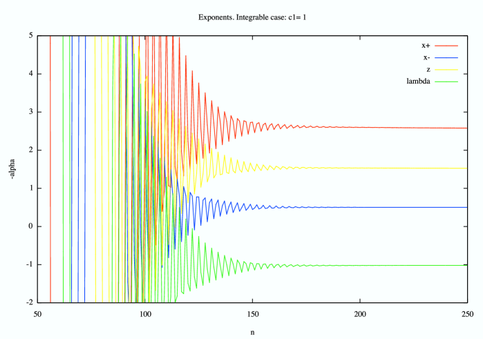
Figure 3: Exponents $-\alpha$ as functions of $n$, p=-1/2, q=3/2.

Note that the curves begin by large oscillations but for $n$ sufficiently large, in the asymptotic regime, the exponents $\alpha$ tend to constants. Comparing with the dominant terms in the binomial formula:

$$\sum n^{\alpha}z^{n}\simeq_{z\to 1}(1-z)^{-1-\alpha}$$

we see that setting $z=\sqrt{t/t_{\infty}}$, we read from figure (3) the various exponents:

$x_{+}(t)$	$\simeq$	$(1-z)^{3/2},$
$x_{-}(t)$	$\simeq$	$(1-z)^{-1/2},$
$z(t)$	$\simeq$	$(1-z)^{1/2},$
$\lambda(t)$	$\simeq$	$(1-z)^{-2},$

The consequence of this observation is that $x_{\pm}(t)$ have Kowalevski expansions around $t_{\infty}$ with indices which are exchanged as compared to those around $t=0$. Hence we know that:

$$x_{+} = -b^{\prime}_{1}\,(t_{\infty}-t)^{{{3}\over{2}}}-{{i\,g\,(t_{\infty}-t)^{2}}\over{2}}-c^{\prime}_{1}\,(t_{\infty}-t)^{{{5}\over{2}}}+\cdots$$

$$x_{-} = -{{{d^{\prime}_{1}}^{2}}\over{b^{\prime}_{1}\,\sqrt{t_{\infty}-t}}}-{{i\,{d^{\prime}_{1}}^{2}\,g}\over{2\,{b^{\prime}_{1}}^{2}}}+{{3\,c^{\prime}_{1}\,{d^{\prime}_{1}}^{2}\,\sqrt{t_{\infty}-t}}\over{{b^{\prime}_{1}}^{2}}}+\cdots$$

where we have introduced a change of sign required by the symmetry $x_{\pm}\to-x_{\mp}$, and the symmetry of the equations of motion under $t\to t_{\infty}-t$. The series expansions have new parameters $b^{\prime}_{1}$, $c^{\prime}_{1}$ and $d^{\prime}_{1}$. In the trigonometric case we see from the explicit formulae that they are equal to the original parameters, see eqs.(LABEL:xplust, LABEL:xmoinst).

We have learned from the previous analysis that the singularities are always of the Kowalevski type, with well-defined exponents. This is perfectly consistent with the exact solution in the trigonometric and elliptic case.

4.2 Non integrable case.

We now explore the region of parameters $-2<p<0,q=2$. We assume that:

$$x_{+}\simeq a_{1}t^{p},\quad x_{-}\simeq b_{1}t^{2},\quad z\simeq c_{1}t^{{p\over 2}+1},\quad c_{1}^{2}=a_{1}b_{1}$$

Notice that $z\to 0$ since we assume $p>-2$, and that $y=-{i\over 2}(x_{+}-x_{-})\simeq-{i\over 2}a_{1}t^{p}$. We see that both terms in eq.(33) for $\lambda$ contribute:

$$\lambda\simeq{mM\over M+m}\left(\left({p\over 2}-1\right)^{2}-{ig\over 2b_{1}}\right){1\over t^{2}}$$

The $x_{\pm}$ equation give:

$$mp(p-1) = {mM\over M+m}\left(\left({p\over 2}-1\right)^{2}-{ig\over 2b_{1}}\right)$$

$$2mb_{1} = img+{mM\over M+m}\left(\left({p\over 2}-1\right)^{2}-{ig\over 2b_{1}}\right)b_{1}$$

Solving for $b_{1}$ we find

$$M=-4m{p-1\over p+2},\quad b_{1}=-{ig\over(p-2)(p+1)}$$

Notice that the mass ratio is positive if $-2<p<0$, and that:

$$\lambda\simeq{mp(p-1)\over t^{2}}$$

For relatively prime integers $r$ and $k$ we set:

$$p=-{r\over k},\quad-2k<-r<-k$$

We perform the Puiseux expansions:

$$x_{+} = t^{-{r\over k}}(a_{1}+a_{2}t^{{1\over k}}+\cdots)$$

$$x_{-} = t^{2}(b_{1}+b_{2}t^{{1\over k}}+\cdots)$$

$$z = t^{-{r\over 2k}+1}(d_{1}+d_{2}t^{{1\over k}}+\cdots)$$

$$\lambda = t^{-2}(l_{1}+l_{2}t^{1\over k}+\cdots)$$

We already know that

$$l_{1}=m{r(r+k)\over k^{2}},\quad a_{1}={d_{1}^{2}\over b_{1}},\quad b_{1}=-{igk^{2}\over(r+2k)(r-k)},\quad M=4m{r+k\over 2k-r}$$

When we plug this into the equations of motion, we get a system of the form:

$${\cal E}_{s}:\hskip 28.45274pt{\cal K}(s)\cdot\pmatrix{a_{s+1}\cr b_{s+1}\cr d_{s+1}\cr l_{s+1}}=\pmatrix{A_{s+1}\cr B_{s+1}\cr D_{s+1}\cr L_{s+1}}$$ (36)

where the Kowalevski matrix reads:

$${\cal K}(s)=\pmatrix{m{(s-r)(s-r-k)\over k^{2}}-l_{1}&0&0&-a_{1}\cr 0&m{(2k+s)(k+s)\over k^{2}}-l_{1}&0&-b_{1}\cr 0&0&M{(k+s-r/2)(s-r/2)\over k^{2}}+l_{1}&d_{1}\cr-b_{1}&-a_{1}&2d_{1}&0}$$

and the right hand side of equation ${\cal E}_{s}$ is given by:

$$A_{s+1} = \sum_{j=2}^{s}a_{j}l_{s+2-j}-img\delta_{s,2k+r}$$

$$B_{s+1} = \sum_{j=2}^{s}b_{j}l_{s+2-j}$$

$$D_{s+1} = -\sum_{j=2}^{s}d_{j}l_{s+2-j}-Mg\delta_{s,k+r/2}$$

$$L_{s+1} = -\sum_{j=2}^{s}d_{j}d_{s+2-j}+\sum_{j=2}^{s}a_{j}b_{s+2-j}$$ (37)

For $s=1$, the quantities $A_{2}$, $B_{2}$, $D_{2}$, $L_{2}$ are meant to be zero. The determinant of the Kowalevski matrix reads:

$$\det({\cal K}(s))=-6m^{2}d_{1}^{2}{(2k+r)\over k^{4}(2k-r)}s(s+k)(s-r)(s+k-r)$$

In order that this determinant vanishes for two positive integer values of $s$, assuming $k>0$, we should have

$$r>0,\quad r-k>0$$

From the equation for $D_{s+1}$ it is natural to choose $r$ even, otherwise the weight $Mg$ would disappear from the problem which is not physical. In order for $r/k$ to be irreducible, we must choose $k$ odd. Setting $r=2r^{\prime}$ we finally get:

$${k\over 2}<r^{\prime}<k,\quad p=-2{r^{\prime}\over k}$$ (38)

When things are setup this way the Kowalevski determinant has two strictly positive integer roots, so that, potentially three arbitrary constants enter the expansion, or the expansion is impossible. Impossibility occurs when the right–hand side of equation ${\cal E}_{s}$ is non vanishing and doesn’t belong to the image of ${\cal K}(s)$ for values of $s$ which are Kowalevski indices. It turns out that in most cases the right–hand side vanishes as we now show.

First, since we want to examine the behavior for $s=r-k$ and $s=r$ we can limit ourselves to studying the system for $s=1,\cdots,r$. In this case the Kronecker deltas in eqs.(37) always vanish. For $\delta_{s,2k+r}$ it is obvious, for $\delta_{s,k+r/2}$ note that, since $k\geq 1+r/2$ we have $k+r/2\geq r+1$. Since the induction starts with $A_{2}=B_{2}=D_{2}=L_{2}=0$, we get, if $s=1$ is not a Kowalevski index that $a_{2}=b_{2}=d_{2}=l_{2}=0$, hence the right–hand side vanishes for the next equation $s=2$. This goes all the way up to $s=r-k$, hence when we hit the first Kowalevski index, it is always with vanishing right–hand side. The existence of a non trivial solution $a_{r-k+1},\cdots,l_{r-k+1}$ is thus guaranteed. Let us assume for the time being that the first Kowalevski index is such that $(r-k)>1$, that is $r\geq k+2$.

As a consequence of this previous step, when $s=r-k+1$ we find that $A_{s+1}$ reduces to $a_{r+k-1}l_{2}$ which also vanishes because $l_{2}=0$. More generally we have $A_{s+1}=\sum_{j=r-k+1}^{s}a_{j}l_{s+2-j}$ which vanishes when $s+2-j<r-k+1$ for all $j$ in the sum, and similarly for the other components. This occurs when $s<2(r-k)$. For $s=2(r-k)$ the right–hand side of equation ${\cal E}_{s}$ doesn’t vanish, and assuming we are not on a Kowalevski index, there is a unique non vanishing solution $a_{2(r-k)+1},\cdots,l_{2(r-k)+1}$. The process continues and it is easy to show by induction that the right–hand side of equation ${\cal E}_{s}$ doesn’t vanish only for $s=n(r-k)$, $n$ positive integer, so non trivial solutions are of the form $a_{n(r-k)+1},\cdots,l_{n(r-k)+1}$. Indeed, to get a non vanishing $a_{j}l_{s+2-j}$ we need to have $j=n(r-k)+1$ and $s+2-j=n^{\prime}(r-k)+1$ so that $s=(n+n^{\prime})(r-k)$. In this case only we have $A_{s+1},\cdots,L_{s+1}$ and thus $a_{s+1},\cdots,l_{s+1}$, non vanishing. This shows that the next non vanishing positions are of the form $(n+n^{\prime})(r-k)+1$ establishing the recurrence.

The second Kowalevski index is $s=r$ and this cannot be of the form $n(r-k)$. Indeed, since $r$ and $k$ are relatively prime, if we have $r=n(r-k)$ we get $(n-1)r=nk$, hence $n=pr$ and $n-1=qk$ for some integers $p$ and $q$. Then $(n-1)r=nk=qkr=prk$ so that $p=q$ and finally $1=p(r-k)$ which is only possible for $p=1$ and $r=k+1$. This is precisely the case we have excluded up to now. As a consequence, when we arrive at the second Kowalevski index $s=r$, the right–hand side of equation ${\cal E}_{s}$ vanishes and there is a non trivial solution, with an extra constant.

We have shown that two new constants of motion always appear for all cases $r=k+3,k+5,\cdots,r=2k-2$. This covers an infinite number of values of the mass ratio $M/m$ for which the Kowalevski criterion is satisfied (with weak Painlevé solutions), but for which the system is presumably non integrable.

Finally we discuss the case $k=r+1$. The first Kowalevski index is $s=1$. In this case the right–hand side vanishes and we have automatically a non trivial solution $[a_{2},b_{2},d_{2},l_{2}]$. From this point, all other solutions of the linear system don’t vanish, and in particular, for the second Kowalevski index, $s=r$, the right–hand side of the system is not trivial. For a solution to exist it must be in the image of ${\cal K}(r)$. Equivalently, let us consider a covector $U=[u_{1},u_{2},u_{3},u_{4}]$ such that $U.{\cal K}(r)=0$. Explicitly:

$$u_{1}=2\,g^{2}\,k^{5},~{}u_{2}=d_{1}^{2}\,(k+1)(3k+1)^{2},~{}u_{3}=i\,d_{1}\,g\,k^{2}\,(k-1)(3k+1)$$

$$u_{4}=-2\,i\,mg\,k\,(k+1)(2k+1)(3k+1)$$

The condition to be satisfied is that the scalar product:

$$W(s)=u_{1}A_{s+1}+u_{2}B_{s+1}+u_{3}D_{s+1}+u_{4}L_{s+1}$$

of this covector and the right–hand side of eq. (36) vanishes for $s=r=k+1$.

For arbitrary $k$ and $s=3,4,...$ we have computed this scalar product $W(s)$, and we have observed that $W(s)$ has a factor $(s-k+1)$. For example we get:

$$W(s=3)=-{mc_{1}^{3}d_{1}^{2}(k-2)(k+1)(2k+1)(3k+1)^{4}\over 4g^{2}k^{5}(k+2)}$$

Note the factor $(k-2)=(r-s)$. For $s=4$ we next get:

$$W(s=4)={imc_{1}^{4}d_{1}^{2}(k-3)(k+1)(2k+1)(3k+1)^{4}P_{6}(k)\over 96g^{3}(k-1)^{2}k^{8}(k+2)^{2}(k+3)}$$

with the factor $(k-3)=(r-s)$. Here $c_{1}$ is the Kowalevski constant which has be introduced at $s=1$, and $P_{6}(k)$ is some polynomial in $k$ of degree 6. The factors in the denominator of course come from similar factors in $\det({\cal K}(s))$. The expression for $s=5$ has the same type of factors in the numerator and denominator, with a more complicated polynomial $P_{7}(k)$ and always a factor $(r-s)$. This behavior is persistent as far as one can compute. The consequence of the presence of the factor $(r-s)$ is that, for any $k$, when we arrive at the second Kowalevski index, $s=r=k+1$, the scalar product $W(k+1)$ vanishes and the linear system is solvable. We can thus state that for all admissible pairs $(k,r)$ the swinging Atwood machine has weak Painlevé expansions depending on the full set of parameters.

For example an interesting case occurs when the mass ratio $M/m=15$ where the system doesn’t look chaotic, see [2]. This case is obtained when $k=19$ and $r=26$. The linear system is solvable in this case, although the new arbitrary constants occur very far from the beginning of the expansion. We shall refrain to exhibit the solution in this case, since it is very bulky, and proceed to show what happens with smaller values of $k$ and $r$.

4.3 Example: the case $k=3$, $r=4$.

When $k=3$ we have necessarily $r=4$. The Kowalevski exponents are $s=0$, $s=1$, $s=4$. The dynamical variables $x_{\pm}$ expand in Puiseux series of $t^{1/3}$ which take the form:

$$x_{+} = t^{-{4\over 3}}\;d_{1}^{2}\left({{10\,i}\over{9\,g\,}}+0\;t^{1\over 3}+{{140\,i\,c_{1}^{2}}\over{729\,g^{3}\,}}t^{{2\over 3}}+{{14000\,c_{1}^{3}}\over{59049\,g^{4}\,}}t^{{3\over 3}}+\right.$$

$$\left.+{{1960\,i\,c_{1}^{4}\,m-32805\,ic_{2}\,g^{4}}\over{91854\,g^{5}\,m}}t^{{4\over 3}}+\cdots\right)$$

$$x_{-} = t^{2}\left(-{{9\,i\,g\,}\over{10}}+c_{1}\,t^{{{1}\over{3}}}+{{7\,i\,c_{1}^{2}\,}\over{30\,g}}t^{{{2}\over{3}}}+{{14\,c_{1}^{3}\,}\over{243\,g^{2}}}t^{3\over 3}+\right.$$

$$\left.+{{\left(96124\,i\,c_{1}^{4}\,m-177147\,i\,c_{2}\,g^{4}\right)}\over{918540\,g^{3}\,m}}\,t^{{{4}\over{3}}}+\cdots\right)$$

This solution depends on 4 arbitrary constants: $t_{0},d_{1},c_{1},c_{2}$ (in the above expansions $t$ should always be understood as $t+t_{0}$). We obtain

$$E\equiv H={{5\,d_{1}^{2}\,\left(13412\,c_{1}^{4}\,m-19683\,c_{2}\,g^{4}\right)}\over{91854\,g^{4}}}$$ (39)

The above constants can be used as local coordinates on phase space. To compute the Poisson brackets of the Kowalevski constants, we proceed as in the previous section considering $\{A_{z}(t),x_{\pm}(t)\}=\pm ix_{\pm}(t)$.

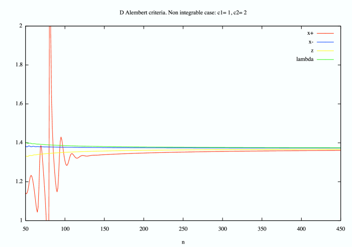
Figure 4: d’Alembert criterium for convergence, $\lim a_{n+1}/a_{n}$ in the non integrable case $c_{1}=1,~{}c_{2}=2$ for $N=450$.

We find:

$$\{t_{0},c_{1}\} = 0$$ (40)

$$\{t_{0},d_{1}\} = 0$$ (41)

$$\{t_{0},c_{2}\} = {{14}\over{15}}\;{1\over d_{1}^{2}}$$ (42)

$$\{d_{1},c_{1}\} = i\;{{3\,g}\over{20\,m}}\;{1\over\,d_{1}}$$ (43)

$$\{d_{1},c_{2}\} = i\;{{13412}\over{32805g^{3}}}\;{c_{1}^{3}\over d_{1}}$$ (44)

$$\{c_{1},c_{2}\} = -i\;{{\left(13412\,c_{1}^{4}\,m-19683\,c_{2}\,g^{4}\right)}\over{65610\,d_{1}^{2}\,g^{3}\,m}}=-i{7g\over 25m}{E\over d_{1}^{4}}$$ (45)

It is remarquable that these six relations ensure the compatibility of an infinite set of relations. One verifies easily the Jacobi identity in spite of the crazy numbers appearing. We can compute the Poisson brackets with $H$

$$\{H,t_{0}\} = 1$$

$$\{H,d_{1}\} = 0$$

$$\{H,c_{1}\} = 0$$

$$\{H,c_{2}\} = 0$$

so that $t_{0}$ is the conjugate variable of $H$ as it should be and the other ones are constants of motion. Notice that $(d_{1}^{2},c_{1})$ is a pair of canonical variables commuting with the pair $(H,t_{0})$. Kowalevski constants are essentially Darboux coordinates.

If there were an extra conserved quantity it would therefore be a function $F(c_{1},c_{2},d_{1})$. The variable $c_{2}$ can be eliminated through $H$ so that we can write as well $F(H,c_{1},d_{1})$.

As in the integrable case we can compute numerically the radius of convergence, and the exponents which nicely fit with the above Kowalevski analysis, as shown in Figure(5).

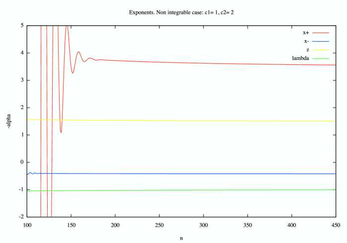
Figure 5: Exponents at singularities in the non integrable case $c_{1}=1,~{}c_{2}=2$ for $N=450$.

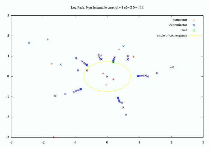
Figure 6: Poles and zeroes of Padé approximant $[M,M+1]$ of $\dot{x}_{+}/x_{+}$ in the non integrable case $c_{1}=1,~{}c_{2}=2$, $M=59$, and $N=119$.

To go further, we also compute the Padé approximants of the series. It is more convenient to consider the logarithmic derivatives $\dot{x}_{\pm}/x_{\pm}$ because the residues of the poles are the exponents. We present the polar decomposition of the $[74,75]$ Padé approximant fo $\dot{x}_{+}/x_{+}$. This shows clearly eight true singularities with residues respectively -1.33 and 2 (up to numerical errors) consistent with the Kowalevski analysis. The other poles having small residues correspond to strings of poles and zeroes representing algebraic branch cuts in the Padé analysis. Note we have set $t=z^{3}$ and we have cancelled the leading $z^{-4}$ at the origin.

$$\dot{x}_{+}/x_{+} = {{2.07+.0366\,i}\over{0.812+0.618\,i+z}}+{{.0295+0.016\,i}\over{0.813+0.622\,i+z}}+\cdots$$

$$+{{2.05-.0136\,i}\over{-0.33+1.04\,i+z}}+{{.0351-.00792\,i}\over{-0.332+1.04\,i+z}}+\cdots$$

$$+{{2.13-.0627\,i}\over{-0.95-0.012\,i+z}}+{{.0725-.0176\,i}\over{-0.954-1.33\times 10^{-2}\,i+z}}+\cdots$$

$$+{{-1.34-.00154\,i}\over{-0.637-0.83\times\,i+z}}+{{-.00711+0.0025\,i}\over{-6.49\times 10^{-1}-8.52\times 10^{-1}\,i+z}}+\cdots$$

$$+{{2.38-0.027\,i}\over{-0.192-0.703\,i+z}}+{{.0281+.0125\,i}\over{-0.192-0.705\,i+z}}+\cdots$$

$$+{{-1.34+3.547\times 10^{-4}\,i}\over{0.175-0.84\,i+z}}+{{-0.0064-3.344\times 10^{-4}\,i}\over{0.177-0.85\,i+z}}+\cdots$$

$$+{{2.29+.114\,i}\over{0.629-0.545\,i+z}}+{{0.077-.0335\,i}\over{0.63-0.547\,i+z}}+\cdots$$

$$+{{-1.34-.00401\,i}\over{1.45-0.586\times 10^{-1}\,i+z}}+{{.0802-.0866\,i}\over{1.62-0.77\,i+z}}+\cdots$$

We see that this structure is very similar to the one we have observed in the integrable elliptic case. This semi–local analysis doesn’t appear to be able to discriminate between the integrable and non integrable cases.

5 Conclusion.

We have studied the swinging Atwood machine, which is believed to be non integrable except for the mass ratio $M/m=3$. We have shown on the explicit solution of the integrable case that the Kowalevski analysis is valid, but requires weak Painlevé expansions. We have extended this weak Painlevé analysis for other values of the mass ratio, and shown that it is valid for an infinite number of cases. Hence this model is remarkable in that it exhibits an infinite number of cases where the Kowalevski analysis works at the price of using Puiseux expansions. However only one of these cases is known to be integrable, while the other ones are believed to be not integrable.

In the cases where Kowalevski expansions are available, we have shown that the constants appearing in these expansions provide Darboux coordinates on an open set of phase space around infinity. The question of integrability of the system therefore reduces to the global nature of this coordinate system $(t_{0},c_{1},c_{2},d_{1})$ on phase space.

On this open set, knowing the Poisson brackets eqs.(40-45), we can try to find the conjugate variable of $t_{0}$. We find that $H$ must be of the form:

$$H=-{15\over 14}d_{1}^{2}c_{2}+h(c_{1},d_{1})$$

The first term agrees with the exact formula in equation (39). The function $h(c_{1},d_{1})$ is not determined but it is of course crucial to have a “good” function $H(\dot{x}_{+},\dot{x}_{-},x_{+},x_{-})$. Clearly we can, in principle, invert locally the system of equations

$$x_{+} = x_{+}(t-t_{0},c_{1},c_{2},d_{1})$$

$$x_{-} = x_{-}(t-t_{0},c_{1},c_{2},d_{1})$$

$$\dot{x}_{+} = \dot{x}_{+}(t-t_{0},c_{1},c_{2},d_{1})$$

$$\dot{x}_{-} = \dot{x}_{-}(t-t_{0},c_{1},c_{2},d_{1})$$

where in the right hand sides we mean the Kowalevski series. In doing so, we will find

$$t-t_{0} = T(x_{+},x_{-},\dot{x}_{+},\dot{x}_{-})$$

$$c_{1} = C_{1}(x_{+},x_{-},\dot{x}_{+},\dot{x}_{-})$$

$$c_{2} = C_{2}(x_{+},x_{-},\dot{x}_{+},\dot{x}_{-})$$

$$d_{1} = D_{1}(x_{+},x_{-},\dot{x}_{+},\dot{x}_{-})$$

but the functions $T,C_{1},C_{2},D_{1}$ will behave in general extremely badly. All this shows that it is in general impossible to make statements about the integrability of the system on the only basis of the Kowalevski analysis. In this context it is remarkable that the global hamiltonian indeed exists, and it is even more remarkable that a second global hamiltonian exists in the integrable case. We see here in a striking way the global nature of integrability.

In the non integrable case, in an attempt to progress beyond the analysis of a single singularity, we have used Padé expansions. In this semi–local analysis, the panorama which appears is still remarkably similar to the one appearing in the elliptic integrable case. Hence Kowalevski analysis is not sufficient to characterize integrability. Nevertheless it is a very non trivial property whose significance remains mysterious.

References

• [1] Tufillaro, N.B., T. A. Abbott, and D. J. Griffiths Swinging Atwood’s Machine, American Journal of Physics, 52 (1984) p.895.
• [2] Tufillaro, N.B. Motions of a swinging Atwood’s machine, Journal de Physique 46 (1985) p.1495.
• [3] Tufillaro, N.B. Collision orbits of a swinging Atwood’s machine, Journal de Physique 46 (1985) p.2053.
• [4] Tufillaro, N.B. Integrable motion of a swinging Atwood’s machine, American Journal of Physics 54 (1986) p.142.
• [5] Casasayas, J., N. B. Tufillaro, and A. Nunes (1989) Infinity manifold of a swinging Atwood’s machine, European Journal of Physics 10 (1989) p.173.
• [6] Casasayas, J, A. Nunes, and N. B. Tufillaro Swinging Atwood’s machine: integrability and dynamics, Journal de Physique 51 (1990) p.1693.
• [7] Nunes, A., J. Casasayas, and N. B. Tufillaro Periodic orbits of the integrable swinging Atwood’s machine, American Journal of Physics 63 (1995) pp.121–126.
• [8] Kowalevski S. Sur le problème de la rotation d’un corps solide autour d’un point fixe, Acta mathematica 12 (1889) pp.177–232
• [9] Yosida H. A criterion for the non-existence of an additional integral in Hamiltonian systems with a homogeneous potential, Physica 29D (1987) pp.122–142.
• [10] Ramani A., Dorizzi B., and Grammaticos B. Painlevé conjecture revisited, Phys. Rev. Lett. 49 (1982) p.1539.
• [11] Babelon O., Bernard D., and Talon M. Introduction to classical integrable systems, Cambridge University Press (2003).
• [12] Adler M., van Moerbeke P., The complex geometry of the Kowalevski–Painlevé analysis, Inventiones mathematicae 97 (1989) 3–51.