Wormhole geometries in $f(R)$ modified theories of gravity

Abstract

In this work, we construct traversable wormhole geometries in the context of $f(R)$ modified theories of gravity. We impose that the matter threading the wormhole satisfies the energy conditions, so that it is the effective stress-energy tensor containing higher order curvature derivatives that is responsible for the null energy condition violation. Thus, the higher order curvature terms, interpreted as a gravitational fluid, sustain these non-standard wormhole geometries, fundamentally different from their counterparts in general relativity. In particular, by considering specific shape functions and several equations of state, exact solutions for $f(R)$ are found.

I Introduction

Various independent high-precision observational data have confirmed with startling evidence that the Universe is undergoing a phase of accelerated expansion observations . Several candidates have been proposed in the literature to explain this phenomenon, ranging from dark energy models to modified theories of gravity. In the latter context, one may assume that at large scales Einstein’s theory of general relativity breaks down, and a more general action describes the gravitational field. The Einstein field equation of general relativity was first derived from an action principle by Hilbert, by adopting a linear function of the scalar curvature, $R$, in the gravitational Lagrangian density. However, there are no a priori reasons to restrict the gravitational Lagrangian to this form, and indeed several generalizations have been proposed. In particular, a more general modification of the Einstein-Hilbert gravitational Lagrangian density involving an arbitrary function of the scalar invariant, $f(R)$, was considered in Bu70 , and further developed in Ke81 .

In this context, a renaissance of $f(R)$ modified theories of gravity has been verified in an attempt to explain the late-time accelerated expansion of the Universe (see Refs. modgrav:review for a review). Earlier interest in $f(R)$ theories was motivated by inflationary scenarios as for instance, in the Starobinsky model, where $f(R)=R-\Lambda+\alpha R^{2}$ was considered Starobinsky:1980te . In fact, it was shown that the late-time cosmic acceleration can be indeed explained within the context of $f(R)$ gravity Carroll:2003wy . Furthermore, the conditions of viable cosmological models have been derived viablemodels , and an explicit coupling of an arbitrary function of $R$ with the matter Lagrangian density has also been explored coupling . Relative to the Solar System regime, severe weak field constraints seem to rule out most of the models proposed so far solartests ; Olmo07 , although viable models do exist solartests2 . In the context of dark matter, the possibility that the galactic dynamics of massive test particles may be understood without the need for dark matter was also considered in the framework of $f(R)$ gravity models darkmatter .

The metric formalism is usually considered in the literature, which consists in varying the action with respect to $g^{\mu\nu}$. However, other alternative approaches have been considered in the literature, namely, the Palatini formalism Palatini ; Sotiriou:2006qn , where the metric and the connections are treated as separate variables; and the metric-affine formalism, where the matter part of the action now depends and is varied with respect to the connection Sotiriou:2006qn . The action for $f(R)$ modified theories of gravity is given by

$$S=\frac{1}{2\kappa}\int d^{4}x\sqrt{-g}\;f(R)+S_{M}(g^{\mu\nu},\psi)\,,$$ (1)

where $\kappa=8\pi G$; throughout this work we consider $\kappa=1$ for notational simplicity. $S_{M}(g^{\mu\nu},\psi)$ is the matter action, defined as $S_{M}=\int d^{4}x\sqrt{-g}\;{\cal L}_{m}(g_{\mu\nu},\psi)$, where ${\cal L}_{m}$ is the matter Lagrangian density, in which matter is minimally coupled to the metric $g_{\mu\nu}$ and $\psi$ collectively denotes the matter fields.

Now, using the metric approach, by varying the action with respect to $g^{\mu\nu}$, provides the following field equation

$$FR_{\mu\nu}-\frac{1}{2}f\,g_{\mu\nu}-\nabla_{\mu}\nabla_{\nu}F+g_{\mu\nu}\Box F=\,T^{m}_{\mu\nu}\,,$$ (2)

where $F\equiv df/dR$. Considering the contraction of Eq. (2), provides the following relationship

$$FR-2f+3\,\Box F=\,T\,,$$ (3)

which shows that the Ricci scalar is a fully dynamical degree of freedom, and $T=T^{\mu}{}_{\mu}$ is the trace of the stress-energy tensor.

In this work, we extend the analysis of static and spherically symmetric spacetimes considered in the literature (for instance, see SSSsolution ), and analyze traversable wormhole geometries in $f(R)$ modified theories of gravity. Wormholes are hypothetical tunnels in spacetime, possibly through which observers may freely traverse. However, it is important to emphasize that these solutions are primarily useful as “gedanken-experiments” and as a theoretician’s probe of the foundations of general relativity. In classical general relativity, wormholes are supported by exotic matter, which involves a stress-energy tensor that violates the null energy condition (NEC) Morris:1988cz ; Visser . Note that the NEC is given by $T_{\mu\nu}k^{\mu}k^{\nu}\geq 0$, where $k^{\mu}$ is any null vector. Thus, it is an important and intriguing challenge in wormhole physics to find a realistic matter source that will support these exotic spacetimes. Several candidates have been proposed in the literature, amongst which we refer to solutions in higher dimensions, for instance in Einstein-Gauss-Bonnet theory EGB1 ; EGB2 , wormholes on the brane braneWH1 ; solutions in Brans-Dicke theory Nandi:1997en ; Anchordoqui:1996jh ; Agnese:1995kd ; wormhole solutions in semi-classical gravity (see Ref. Garattini:2007ff and references therein); exact wormhole solutions using a more systematic geometric approach were found Boehmer:2007rm ; geometries supported by equations of state responsible for the cosmic acceleration phantomWH , solutions in conformal Weyl gravity were found Weylgrav , and thin accretion disk observational signatures were also explored Harko:2008vy , etc (see Refs. Lemos:2003jb ; Lobo:2007zb for more details and Lobo:2007zb for a recent review).

Thus, we explore the possibility that wormholes be supported by $f(R)$ modified theories of gravity. It is an effective stress energy, which may be interpreted as a gravitational fluid, that is responsible for the null energy condition violation, thus supporting these non-standard wormhole geometries, fundamentally different from their counterparts in general relativity. We also impose that the matter threading the wormhole satisfies the energy conditions.

This paper is organized in the following manner: In Sec. II, the spacetime metric, the effective field equations and the energy condition violations in the context of $f(R)$ modified theories of gravity are analyzed in detail. In Sec. III, specific solutions are explored, and we conclude in Sec. IV.

II Wormhole geometries in $f(R)$ gravity

II.1 Spacetime metric and gravitational field equations

Consider the wormhole geometry given by the following static and spherically symmetric metric

$$ds^{2}=-e^{2\Phi(r)}dt^{2}+\frac{dr^{2}}{1-b(r)/r}+r^{2}\,(d\theta^{2}+\sin^{2}{\theta}\,d\phi^{2})\,,$$ (4)

where $\Phi(r)$ and $b(r)$ are arbitrary functions of the radial coordinate, $r$, denoted as the redshift function, and the shape function, respectively Morris:1988cz . The radial coordinate $r$ is non-monotonic in that it decreases from infinity to a minimum value $r_{0}$, representing the location of the throat of the wormhole, where $b(r_{0})=r_{0}$, and then it increases from $r_{0}$ back to infinity.

A fundamental property of a wormhole is that a flaring out condition of the throat, given by $(b-b^{\prime}r)/b^{2}>0$, is imposed Morris:1988cz , and at the throat $b(r_{0})=r=r_{0}$, the condition $b^{\prime}(r_{0})<1$ is imposed to have wormhole solutions. It is precisely these restrictions that impose the NEC violation in classical general relativity. Another condition that needs to be satisfied is $1-b(r)/r>0$. For the wormhole to be traversable, one must demand that there are no horizons present, which are identified as the surfaces with $e^{2\Phi}\rightarrow 0$, so that $\Phi(r)$ must be finite everywhere. In the analysis outlined below, we consider that the redshift function is constant, $\Phi^{\prime}=0$, which simplifies the calculations considerably, and provide interesting exact wormhole solutions (If $\Phi^{\prime}\neq 0$, the field equations become forth order differential equations, and become quite intractable).

The trace equation (3) can be used to simplify the field equations and then can be kept as a constraint equation. Thus, substituting the trace equation into Eq. (2), and re-organizing the terms we end up with the following gravitational field equation

$$G_{\mu\nu}\equiv R_{\mu\nu}-\frac{1}{2}R\,g_{\mu\nu}=T^{{\rm eff}}_{\mu\nu}\,,$$ (5)

where the effective stress-energy tensor is given by $T^{{\rm eff}}_{\mu\nu}=T^{(c)}_{\mu\nu}+\tilde{T}^{(m)}_{\mu\nu}$. The term $\tilde{T}^{(m)}_{\mu\nu}$ is given by

$$\tilde{T}^{(m)}_{\mu\nu}=T^{(m)}_{\mu\nu}/F\,,$$ (6)

and the curvature stress-energy tensor, $T^{(c)}_{\mu\nu}$, is defined as

$$T^{(c)}_{\mu\nu}=\frac{1}{F}\left[\nabla_{\mu}\nabla_{\nu}F-\frac{1}{4}g_{\mu\nu}\left(RF+\Box F+T\right)\right]\,.$$ (7)

It is also interesting to consider the conservation law for the above curvature stress-energy tensor. Taking into account the Bianchi identities, $\nabla^{\mu}G_{\mu\nu}=0$, and the diffeomorphism invariance of the matter part of the action, which yields $\nabla^{\mu}T^{(m)}_{\mu\nu}=0$, we verify that the effective Einstein field equation provides the following conservation law

$$\nabla^{\mu}T^{(c)}_{\mu\nu}=\frac{1}{F^{2}}T^{(m)}_{\mu\nu}\nabla^{\mu}F\,.$$ (8)

Relative to the matter content of the wormhole, we impose that the stress-energy tensor that threads the wormhole satisfies the energy conditions, and is given by the following anisotropic distribution of matter

$$T_{\mu\nu}=(\rho+p_{t})U_{\mu}\,U_{\nu}+p_{t}\,g_{\mu\nu}+(p_{r}-p_{t})\chi_{\mu}\chi_{\nu}\,,$$ (9)

where $U^{\mu}$ is the four-velocity, $\chi^{\mu}$ is the unit spacelike vector in the radial direction, i.e., $\chi^{\mu}=\sqrt{1-b(r)/r}\,\delta^{\mu}{}_{r}$. $\rho(r)$ is the energy density, $p_{r}(r)$ is the radial pressure measured in the direction of $\chi^{\mu}$, and $p_{t}(r)$ is the transverse pressure measured in the orthogonal direction to $\chi^{\mu}$. Taking into account the above considerations, the stress-energy tensor is given by the following profile: $T^{\mu}{}_{\nu}={\rm diag}[-\rho(r),p_{r}(r),p_{t}(r),p_{t}(r)]$.

Thus, the effective field equation (5) provides the following relationships

$$\frac{b^{\prime}}{r^{2}} = \frac{\rho}{F}+\frac{H}{F}\,,$$ (10)

$$-\frac{b}{r^{3}} = \frac{p_{r}}{F}+\frac{1}{F}\Bigg{\{}\left(1-\frac{b}{r}\right)\times$$ (11)

$$\times\left[F^{\prime\prime}-F^{\prime}\frac{b^{\prime}r-b}{2r^{2}(1-b/r)}\right]-H\Bigg{\}}\,,$$

$$-\frac{b^{\prime}r-b}{2r^{3}} = \frac{p_{t}}{F}+\frac{1}{F}\left[\left(1-\frac{b}{r}\right)\frac{F^{\prime}}{r}-H\right]\,,$$ (12)

where the prime denotes a derivative with respect to the radial coordinate, $r$. The term $H=H(r)$ is defined as

$$H(r)=\frac{1}{4}\left(FR+\Box F+T\right)\,,$$ (13)

for notational simplicity. The curvature scalar, $R$, is given by

$$R = \frac{2b^{\prime}}{r^{2}}\,,$$ (14)

and $\Box F$ is provided by the following expression

$$\Box F=\left(1-\frac{b}{r}\right)\left[F^{\prime\prime}-\frac{b^{\prime}r-b}{2r^{2}(1-b/r)}\,F^{\prime}+\frac{2F^{\prime}}{r}\right]\,.$$ (15)

Note that the gravitational field equations (10)-(12), can be reorganized to yield the following relationships:

$$\rho = \frac{Fb^{\prime}}{r^{2}}\,,$$ (16)

$$p_{r} = -\frac{bF}{r^{3}}+\frac{F^{\prime}}{2r^{2}}(b^{\prime}r-b)-F^{\prime\prime}\left(1-\frac{b}{r}\right)\,,$$ (17)

$$p_{t} = -\frac{F^{\prime}}{r}\left(1-\frac{b}{r}\right)+\frac{F}{2r^{3}}(b-b^{\prime}r)\,,$$ (18)

which are the generic expressions of the matter threading the wormhole, as a function of the shape function and the specific form of $F(r)$. Thus, by specifying the above functions, one deduces the matter content of the wormhole.

One may now adopt several strategies to solve the field equations. For instance, if $b(r)$ is specified, and using a specific equation of state $p_{r}=p_{r}(\rho)$ or $p_{t}=p_{t}(\rho)$ one can obtain $F(r)$ from the gravitational field equations and the curvature scalar in a parametric form, $R(r)$, from its definition via the metric. Then, once $T=T^{\mu}{}_{\mu}$ is known as a function of $r$, one may in principle obtain $f(R)$ as a function of $R$ from Eq. (3).

II.2 Energy condition violations

A fundamental point in wormhole physics is the energy condition violations, as mentioned above. However, a subtle issue needs to be pointed out in modified theories of gravity, where the gravitational field equations differ from the classical relativistic Einstein equations. More specifically, we emphasize that the energy conditions arise when one refers back to the Raychaudhuri equation for the expansion where a term $R_{\mu\nu}k^{\mu}k^{\nu}$ appears, with $k^{\mu}$ any null vector. The positivity of this quantity ensures that geodesic congruences focus within a finite value of the parameter labelling points on the geodesics. However, in general relativity, through the Einstein field equation one can write the above condition in terms of the stress-energy tensor given by $T_{\mu\nu}k^{\mu}k^{\nu}\geq 0$. In any other theory of gravity, one would require to know how one can replace $R_{\mu\nu}$ using the corresponding field equations and hence using matter stresses. In particular, in a theory where we still have an Einstein-Hilbert term, the task of evaluating $R_{\mu\nu}k^{\mu}k^{\nu}$ is trivial. However, in $f(R)$ modified theories of gravity under consideration, things are not so straightforward.

Now the positivity condition, $R_{\mu\nu}k^{\mu}k^{\nu}\geq 0$, in the Raychaudhuri equation provides the following form for the null energy condition $T^{{\rm eff}}_{\mu\nu}k^{\mu}k^{\nu}\geq 0$, through the modified gravitational field equation (5), and it this relationship that will be used throughout this work. For this case, in principle, one may impose that the matter stress-energy tensor satisfies the energy conditions and the respective violations arise from the higher derivative curvature terms $T^{(c)}_{\mu\nu}$. Another approach to the energy conditions considers in taking the condition $T_{\mu\nu}k^{\mu}k^{\nu}\geq 0$ at face value. Note that this is useful as using local Lorentz transformations it is possible to show that the above condition implies that the energy density is positive in all local frames of reference. However, if the theory of gravity is chosen to be non-Einsteinian, then the assumption of the above condition does not necessarily imply focusing of geodesics. The focusing criterion is different and will follow from the nature of $R_{\mu\nu}k^{\mu}k^{\nu}$.

Thus, considering a radial null vector, the violation of the NEC, i.e., $T_{\mu\nu}^{{\rm eff}}\,k^{\mu}k^{\nu}<0$ takes the following form

$$\rho^{{\rm eff}}+p_{r}^{{\rm eff}}=\frac{\rho+p_{r}}{F}+\frac{1}{F}\left(1-\frac{b}{r}\right)\left[F^{\prime\prime}-F^{\prime}\frac{b^{\prime}r-b}{2r^{2}(1-b/r)}\right],$$ (19)

where $\rho^{{\rm eff}}+p_{r}^{{\rm eff}}<0$. Using the gravitational field equations, inequality (19) takes the familiar form

$$\rho^{{\rm eff}}+p_{r}^{{\rm eff}}=\frac{b^{\prime}r-b}{r^{3}}\,,$$ (20)

which is negative by taking into account the flaring out condition, i.e., $(b^{\prime}r-b)/b^{2}<0$, considered above.

At the throat, one has the following relationship

$$\rho^{{\rm eff}}+p_{r}^{{\rm eff}}|_{r_{0}}=\frac{\rho+p_{r}}{F}\Big{|}_{r_{0}}+\frac{1-b^{\prime}(r_{0})}{2r_{0}}\frac{F^{\prime}}{F}\Big{|}_{r_{0}}<0\,.$$ (21)

It is now possible to find the following generic relationships for $F$ and $F^{\prime}$ at the throat: $F^{\prime}_{0}<-2r_{0}(\rho+p_{r})|_{r_{0}}/(1-b^{\prime})$ if $F>0$; and $F^{\prime}_{0}>-2r_{0}(\rho+p_{r})|_{r_{0}}/(1-b^{\prime})$ if $F<0$.

Consider that the matter threading the wormhole obeys the energy conditions. To this effect, imposing the weak energy condition (WEC), given by $\rho\geq 0$ and $\rho+p_{r}\geq 0$, then Eqs. (16)-(17) yield the following inequalities:

$$\frac{Fb^{\prime}}{r^{2}}\geq 0\,,$$ (22)

$$\frac{(2F+rF^{\prime})(b^{\prime}r-b)}{2r^{2}}-F^{\prime\prime}\left(1-\frac{b}{r}\right)\geq 0\,,$$ (23)

respectively.

Thus, if one imposes that the matter threading the wormhole satisfies the energy conditions, we emphasize that it is the higher derivative curvature terms that sustain the wormhole geometries. Thus, in finding wormhole solutions it is fundamental that the functions $f(R)$ obey inequalities (19) and (22)-(23).

III Specific solutions

In this section, we are mainly interested in adopting the strategy of specifying the shape function $b(r)$, which yields the curvature scalar in a parametric form, $R(r)$, from its definition via the metric, given by Eq. (14). Then, using a specific equation of state $p_{r}=p_{r}(\rho)$ or $p_{t}=p_{t}(\rho)$, one may in principle obtain $F(r)$ from the gravitational field equations. Finally, once $T=T^{\mu}{}_{\mu}$ is known as a function of $r$, one may in principle obtain $f(R)$ as a function of $R$ from Eq. (3).

III.1 Traceless stress-energy tensor

An interesting equation of state is that of the traceless stress-energy tensor, which is usually associated to the Casimir effect, with a massless field. Note that the Casimir effect is sometimes theoretically invoked to provide exotic matter to the system considered at hand. Thus, taking into account the traceless stress-energy tensor, $T=-\rho+p_{r}+2p_{t}=0$, provides the following differential equation

$$F^{\prime\prime}\left(1-\frac{b}{r}\right)-\frac{b^{\prime}r+b-2r}{2r^{2}}F^{\prime}-\frac{b^{\prime}r-b}{2r^{3}}F=0\,.$$ (24)

In principle, one may deduce $F(r)$ by imposing a specific shape function, and inverting Eq. (14), i.e., $R(r)$, to find $r(R)$, the specific form of $f(R)$ may be found from the trace equation (3).

For instance, consider the specific shape function given by $b(r)=r_{0}^{2}/r$. Thus, Eq. (24) provides the following solution

$$F(r) = C_{1}\sinh\left[\sqrt{2}\,\arctan\left(\frac{r_{0}}{\sqrt{r^{2}-r_{0}^{2}}}\right)\right]$$ (25)

$$+C_{2}\cosh\left[\sqrt{2}\,\arctan\left(\frac{r_{0}}{\sqrt{r^{2}-r_{0}^{2}}}\right)\right]\,.$$

The stress-energy tensor profile threading the wormhole is given by the following relationships

$$\rho(r) = -\frac{r_{0}^{2}}{r^{4}}\Bigg{\{}C_{1}\sinh\left[\sqrt{2}\,\arctan\left(\frac{r_{0}}{\sqrt{r^{2}-r_{0}^{2}}}\right)\right]+C_{2}\cosh\left[\sqrt{2}\,\arctan\left(\frac{r_{0}}{\sqrt{r^{2}-r_{0}^{2}}}\right)\right]\Bigg{\}}\,,$$ (26)

$$p_{r}(r) = -\frac{r_{0}}{r^{4}}\Bigg{\{}\left(2C_{2}\sqrt{2(r^{2}-r_{0}^{2})}+3r_{0}C_{1}\right)\sinh\left[\sqrt{2}\,\arctan\left(\frac{r_{0}}{\sqrt{r^{2}-r_{0}^{2}}}\right)\right]$$ (27)

$$+\left(2C_{1}\sqrt{2(r^{2}-r_{0}^{2})}+3r_{0}C_{2}\right)\cosh\left[\sqrt{2}\,\arctan\left(\frac{r_{0}}{\sqrt{r^{2}-r_{0}^{2}}}\right)\right]\Bigg{\}}\,,$$

$$p_{t}(r) = \frac{r_{0}}{r^{4}}\Bigg{\{}\left(C_{2}\sqrt{2(r^{2}-r_{0}^{2})}+r_{0}C_{1}\right)\sinh\left[\sqrt{2}\,\arctan\left(\frac{r_{0}}{\sqrt{r^{2}-r_{0}^{2}}}\right)\right]$$ (28)

$$+\left(C_{1}\sqrt{2(r^{2}-r_{0}^{2})}+r_{0}C_{2}\right)\cosh\left[\sqrt{2}\,\arctan\left(\frac{r_{0}}{\sqrt{r^{2}-r_{0}^{2}}}\right)\right]\Bigg{\}}\,.$$

One may now impose that the above stress-energy tensor satisfies the WEC, which is depicted in Fig. 1, by considering the values $C_{1}=0$ and $C_{2}=-1$.

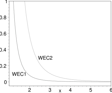
Figure 1: The stress-energy tensor satisfying the WEC, for the specific case of the traceless stress-energy tensor equation of state, and for the values $C_{1}=0$ and $C_{2}=-1$. We have considered the dimensionless quantities ${\rm WEC}1=r_{0}^{2}\rho$, ${\rm WEC}2=r_{0}^{2}(\rho+p_{r})$ and $x=r/r_{0}$.

For the specific shape function considered above, the Ricci scalar, Eq. (14), provides $R=-2r_{0}^{2}/r^{4}$ and is now readily inverted to give $r=(-2r_{0}^{2}/R)^{1/4}$. It is also convenient to define the Ricci scalar at the throat, and its inverse provides $r_{0}=(-2/R_{0})^{1/2}$. Substituting these relationships into the consistency equation (3), the specific form $f(R)$ is given by

$$f(R) = -R\Bigg{\{}C_{1}\sinh\left[\sqrt{2}\arctan\left(\frac{1}{\sqrt{\left(\frac{R_{0}}{R}\right)^{1/2}-1}}\right)\right]$$ (29)

$$+C_{2}\cosh\left[\sqrt{2}\arctan\left(\frac{1}{\sqrt{\left(\frac{R_{0}}{R}\right)^{1/2}-1}}\right)\right]\Bigg{\}}\,,$$

which is depicted in the Fig. 2, by imposing the values $C_{1}=0$ and $C_{2}=-1$.

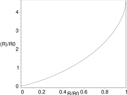
Figure 2: The specific form of $f(R)$, for the specific case of the traceless stress-energy tensor equation of state, by imposing the values $C_{1}=0$ and $C_{2}=-1$. The range is given by $0\leq R/R_{0}\leq 1$.

III.2 Specific equation of state: $p_{t}=\alpha\rho$

Many of the equations of state considered in the literature involving the radial pressure and the energy density, such as the linear equation of state $p_{r}=\alpha\rho$, provide very complex differential equations, so that it is extremely difficult to find exact solutions. This is due to the presence of the term $F^{\prime\prime}$ in $p_{r}$. Indeed, even considering isotropic pressures does not provide an exact solution. Now, things are simplified if one considers an equation of state relating the tangential pressure and the energy density, so that the radial pressure is determined through Eq. (17). For instance, consider the equation of state $p_{t}=\alpha\rho$, which provides the following differential equation:

$$F^{\prime}\left(1-\frac{b}{r}\right)-\frac{F}{2r^{2}}\left[b-b^{\prime}r(1+2\alpha)\right]=0\,.$$ (30)

In principle, as mentioned above one may deduce $F(r)$ by imposing a specific shape function, and inverting Eq. (14), i.e., $R(r)$, to find $r(R)$, the specific form of $f(R)$ may be found from the trace equation (3). In the following analysis we consider several interesting shape functions usually applied in the literature.

1. Specific shape function: $b(r)=r_{0}^{2}/r$

First, we consider the case of $b(r)=r_{0}^{2}/r$, so that Eq. (30) yields the following solution

$$F(r)=C_{1}\left(1-\frac{r_{0}^{2}}{r^{2}}\right)^{\frac{1}{2}+\frac{\alpha}{2}}\,.$$ (31)

The gravitational field equations, (16)-(18), provide the stress-energy tensor threading the wormhole, given by the following relationships

$$p_{r}(r) = \frac{C_{1}r_{0}^{2}}{r^{6}}\left(1-\frac{r_{0}^{2}}{r^{2}}\right)^{-\frac{1}{2}+\frac{\alpha}{2}}\times$$ (32)

$$\times\left[2(r^{2}-r_{0}^{2})+3\alpha r^{2}-4r_{0}^{2}\alpha-r_{0}^{2}\alpha^{2}\right]\,,$$

$$p_{t}(r) = \alpha\rho(r)=-\frac{C_{1}r_{0}^{2}\alpha}{r^{4}}\left(1-\frac{r_{0}^{2}}{r^{2}}\right)^{\frac{1}{2}+\frac{\alpha}{2}}\,.$$ (33)

One may now impose that the above stress-energy tensor satisfies the WEC, which is depicted in Fig. 3, by imposing the values $C_{1}=-1$ and $\alpha=-1$.

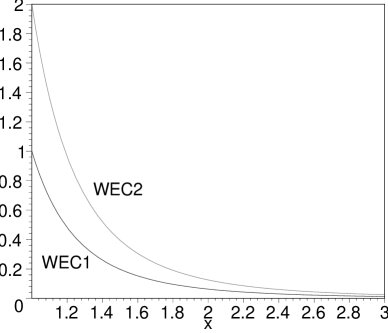
Figure 3: The stress-energy tensor satisfies the WEC, for the specific case of the equation of state $p_{t}=\alpha\rho$ and considering the form function $b(r)=r_{0}^{2}/r$. We have imposed the values $C_{1}=-1$ and $\alpha=-1$, and considered the dimensionless quantities ${\rm WEC}1=r_{0}^{2}\rho$, ${\rm WEC}2=r_{0}^{2}(\rho+p_{r})$ and $x=r/r_{0}$.

As in the previous case of the traceless stress-energy tensor, the Ricci scalar, Eq. (14), is given by $R=-2r_{0}^{2}/r^{4}$ and its inverse provides $r=(-2r_{0}^{2}/R)^{1/4}$. The inverse of the Ricci scalar evaluated at the throat inverse is given by $r_{0}=(-2/R_{0})^{1/2}$. Substituting these relationships into the consistency relationship (3), provides the specific form of $f(R)$, which is given by

$$f(R) = C_{1}R\left(1-\sqrt{\frac{R}{R_{0}}}\right)^{\frac{\alpha}{2}-\frac{1}{2}}\times$$ (34)

$$\times\left[\sqrt{\frac{R}{R_{0}}}(\alpha^{2}+2\alpha+2)+(\alpha+2)\right]\,.$$

This function is depicted in Fig. 4 as $f(R)/R_{0}$ as a function as $R/R_{0}$, for the values $C_{1}=-1$ and $\alpha=-1$.

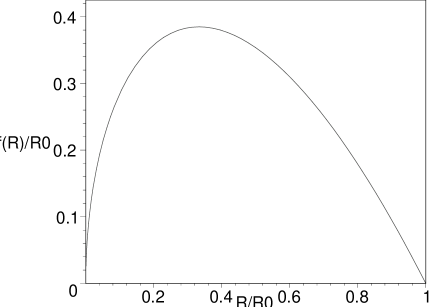
Figure 4: The profile of $f(R)$ is depicted for the specific case of the equation of state $p_{t}=\alpha\rho$ and considering the form function $b(r)=r_{0}^{2}/r$. The values $C_{1}=-1$ and $\alpha=-1$ have been imposed, with the range given by $0\leq R/R_{0}\leq 1$.

2. Specific shape function: $b=\sqrt{r_{0}r}$

Consider now the case of $b=\sqrt{r_{0}r}$, so that Eq. (30) yields the following solution

$$F(r)=C_{1}\left(1-\sqrt{\frac{r_{0}}{r}}\,\right)^{\frac{1}{2}-\alpha}\,.$$ (35)

The stress-energy tensor profile threading the wormhole is given by the following relationships

$$p_{t}(r) = \alpha\rho(r)=\frac{C_{1}\alpha}{2r^{2}}\frac{\left(1-\sqrt{\frac{r_{0}}{r}}\right)^{\frac{1}{2}-\alpha}}{\sqrt{\frac{r_{0}}{r}}}\,,$$ (36)

$$p_{r}(r) = -\frac{C_{1}r_{0}}{16r^{3}}\left(1-\sqrt{\frac{r_{0}}{r}}\right)^{-\frac{3}{2}-\alpha}\times$$ (37)

$$\times\bigg{[}10\sqrt{\frac{r}{r_{0}}}+\sqrt{\frac{r_{0}}{r}}\left(14\alpha+10\right)+\left(4\alpha^{2}-26\alpha+5\right)\bigg{]}\,.$$

Rather than consider plots of the WEC as before, we note that it is possible to impose various specific values of $C_{1}$ and $\alpha$ that do indeed satisfy the WEC.

Following the recipe prescribed above, the Ricci scalar is given by $R=\sqrt{r_{0}}/r^{5/2}$ and is readily inverted to provide $r=(\sqrt{r_{0}}/R)^{2/5}$. The inverse of the Ricci scalar at the throat provides $r_{0}=1/\sqrt{R_{0}}$. Substituting these relationships into the consistency relationship (3), the specific form $f(R)$ is finally given by

$$f(R) = -\frac{1}{8}\frac{C_{1}}{R^{\frac{2}{5}}-2\left(RR_{0}\right)^{\frac{1}{5}}+R_{0}^{\frac{2}{5}}}\Bigg{\{}\left(R_{0}^{\frac{1}{5}}-R^{\frac{1}{5}}\right)^{\frac{1}{2}-\alpha}R^{\frac{3-2\alpha}{10}}R_{0}^{\frac{-21+10\alpha}{40}}\times$$ (38)

$$\times\left[-8RR_{0}^{\frac{2}{5}}+\right(11+10\alpha\left)R^{\frac{4}{5}}R_{0}^{\frac{3}{5}}+\right(2-22\alpha+4\alpha^{2}\left)R^{\frac{3}{5}}R_{0}^{\frac{4}{5}}+\left(-5+12\alpha-4\alpha^{2}\right)R^{\frac{2}{5}}R_{0}\right]\Bigg{\}}\,.$$

3. Specific shape function: $b(r)=r_{0}+\gamma^{2}r_{0}(1-r_{0}/r)$

Finally, it is also of interest to consider the specific shape function given by $b(r)=r_{0}+\gamma^{2}r_{0}(1-r_{0}/r)$, with $0<\gamma<1$, so that Eq. (30) provides the following solution

$$F(r) = C_{1}\left(r-\gamma^{2}r_{0}\right)^{\frac{1}{2}\frac{\gamma^{2}-2\alpha-1}{\gamma^{2}-1}}$$ (39)

$$r^{-(\alpha+1)}\left(r-r_{0}\right)^{\frac{1}{2}\frac{\gamma^{2}(1+2\alpha)-1}{\gamma^{2}-1}}$$

It is useful to write the last equation in the form $F(r)=C_{1}X^{u}r^{-(\alpha+1)}Y^{v}$, where $X,\,Y,\,u,\,v$ are defined as

$$X=r-\gamma^{2}r_{0}\,,\qquad Y=r-r_{0}\,,$$

$$u=\frac{\gamma^{2}-2\alpha-1}{2(\gamma^{2}-1)}\,,\qquad v=\frac{\gamma^{2}(1+2\alpha)-1}{2(\gamma^{2}-1)}\,.$$

Thus, the stress energy tensor profile threading the wormhole is given by the following expressions:

$$p_{r}(r) = \frac{C_{1}}{2r^{3}}\Bigg{\{}X^{u}Y^{v}\bigg{[}r^{-\alpha}\left(2\alpha^{2}+6\alpha+4\right)+r^{-(1+\alpha)}r_{0}\left(-7\alpha+2\alpha^{2}\gamma^{2}-3\gamma^{2}-7\alpha\gamma^{2}-2\alpha^{2}-3\right)$$

$$+r^{-(2+\alpha)}r_{0}^{2}\gamma^{2}\left(10\alpha^{2}+4\right)\bigg{]}+X^{u}Y^{v-1}\bigg{[}r^{-\alpha}r_{0}v\left(-\gamma^{2}(5+4\alpha)-\alpha-5\right)+4r^{1-\alpha}v\left(1+\alpha\right)$$

$$+r^{-(1+\alpha)}r_{0}^{2}\gamma^{2}v\left(4\alpha+6\right)\bigg{]}+X^{u}Y^{v-2}\bigg{[}2r^{-\alpha}r_{0}\gamma^{2}v\left(v-\alpha\right)+2r^{1-\alpha}r_{0}v\left(-v+\gamma^{2}+1\right)$$

$$+2r^{2-\alpha}v\left(v+1\right)\bigg{]}+X^{u-1}Y^{v}\bigg{[}r^{-\alpha}r_{0}u\left(4\alpha+5\right)\left(\gamma^{2}+1\right)-4r^{1-\alpha}\left(u-\alpha\right)$$

$$-r^{-(1+\alpha)}r_{0}^{2}\gamma^{2}u\left(4\alpha-6\right)\bigg{]}+X^{u-2}Y^{v}\big{[}2r^{-\alpha}r_{0}^{2}\gamma^{2}u\left(u-1\right)+2r^{1-\alpha}r_{0}u\left(1-u\right)+2r^{2-\alpha}u\left(u-1\right)\bigg{]}$$

$$+X^{u-1}Y^{v-1}\bigg{[}-4r^{-\alpha}r_{0}^{2}\gamma^{2}uv+4r^{1-\alpha}r_{0}uv\left(\gamma^{2}+1\right)-4r^{2-\alpha}uv\bigg{]}\Bigg{\}}\,,$$

$$p_{t}(r) = \alpha\rho=C_{1}\alpha\gamma^{2}r_{0}^{2}X^{u}r^{-(5+\alpha)}Y^{v}\,.$$ (41)

As in the previous example, we will not depict the plot of the functions, but simply note in passing that one may impose specific values for the constants $\alpha$ and $C_{1}$ in order to satisfy the WEC.

The Ricci scalar, Eq. (14), provides $R=2\gamma^{2}r_{0}^{2}/r^{4}$ and is now readily inverted to give $r=(2\gamma^{2}r_{0}^{2}/R)^{1/4}$. The Ricci scalar at the throat is given by $R_{0}=2\gamma^{2}/r_{0}^{2}$, and its inverse provides $r_{0}=\gamma\sqrt{2/R_{0}}$. Substituting these relationships into the consistency relationship (3), the specific form $f(R)$ is given by

$$f(R) = \frac{C_{1}R}{2}\frac{\left(R_{0}R\right)^{\frac{(\alpha+1)}{4}}}{\gamma^{2}-\left(\frac{R_{0}}{R}\right)^{\frac{1}{4}}(\gamma^{2}+1)+\left(\frac{R_{0}}{R}\right)^{\frac{1}{2}}}\left[\frac{\left(\frac{R_{0}}{R}\right)^{\frac{1}{4}}-\gamma^{2}}{R_{0}^{\frac{1}{2}}}\right]^{\frac{1}{2}\frac{\gamma^{2}-2\alpha-1}{\gamma^{2}-1}}\left[\frac{\left(\frac{R_{0}}{R}\right)^{\frac{1}{4}}-1}{R_{0}^{\frac{1}{2}}}\right]^{\frac{1}{2}\frac{\gamma^{2}(1-2\alpha)-1}{\gamma^{2}-1}}\times$$ (42)

$$\left[2\gamma^{2}(\alpha^{2}+2\alpha+2)-\left(\frac{R_{0}}{R}\right)^{\frac{1}{4}}(3\alpha+4)(\gamma^{2}+1)+\left(\frac{R_{0}}{R}\right)^{\frac{1}{2}}(2\alpha+4)\right]\,.$$

IV Summary and Discussion

In general relativity, the NEC violation is a fundamental ingredient of static traversable wormholes. Despite this fact, it was shown that for time-dependent wormhole solutions the null energy condition and the weak energy condition can be avoided in certain regions and for specific intervals of time at the throat dynamicWH . Nevertheless, in certain alternative theories to general relativity, taking into account the modified Einstein field equation, one may impose in principle that the stress energy tensor threading the wormhole satisfies the NEC. However, the latter is necessarily violated by an effective total stress energy tensor. This is the case, for instance, in braneworld wormhole solutions, where the matter confined on the brane satisfies the energy conditions, and it is the local high-energy bulk effects and nonlocal corrections from the Weyl curvature in the bulk that induce a NEC violating signature on the brane braneWH1 . Another particularly interesting example is in the context of the $D$-dimensional Einstein-Gauss-Bonnet theory of gravitation EGB1 , where it was shown that the weak energy condition can be satisfied depending on the parameters of the theory.

In this work, we have explored the possibility that wormholes be supported by $f(R)$ modified theories of gravity. We imposed that the matter threading the wormhole satisfies the energy conditions, and it is the higher order curvature derivative terms, that may be interpreted as a gravitational fluid, that support these non-standard wormhole geometries, fundamentally different from their counterparts in general relativity. In the analysis outlined above, we considered a constant redshift function, which simplified the calculations considerably, yet provides interesting enough exact solutions. One may also generalize the results of this paper by considering $\Phi^{\prime}\neq 0$, although the field equations become forth order differential equations, and become quite intractable. The strategy adopted to solve the field equations was essentially to specify $b(r)$, and considering specific equation of state, the function $F(r)$ was deduced from the gravitational field equations, while the curvature scalar in a parametric form, $R(r)$, was obtained from its definition via the metric. Then, deducing $T=T^{\mu}{}_{\mu}$ as a function of $r$, exact solutions of $f(R)$ as a function of $R$ from the trace equation were found.

Furthermore, we note that $f(R)$ modified theories of gravity are equivalent to a Brans-Dicke theory with a coupling parameter $w=0$, and a specific potential related to the function $f(R)$ and its derivative. In this context, it was shown that static wormhole solutions in the vacuum Brans-Dicke theory only exist in a narrow interval of the coupling parameter Nandi:1997en , namely, $-3/2<w<-4/3$. However, we point out that this result is only valid for vacuum solutions and for a specific choice of an integration constant of the field equations given by $C(w)=-1/(w+2)$. The latter relationship was derived on the basis of a post-Newtonian weak field approximation, and it is important to emphasize that there is no reason for it to hold in the presence of compact objects with strong gravitational fields.

Another issue that needs to be mentioned, is that the above-mentioned interval imposed on $w$ was obtained by considering the violation of the WEC (recall that the WEC imposes $\rho\geq 0$ and $\rho+p_{r}\geq 0$). Now the authors in Nandi:1997en obtained the respective constraints on $w$ by considering negative energy densities, i.e., $\rho<0$. This is not a necessary condition, as one may consider positive energy densities and in alternative impose the condition $\rho+p_{r}<0$, which violates the WEC, and consequently the NEC. Note that this is justified as the fundamental ingredient in wormhole physics is the violation of the NEC, and not the imposition of negative energy densities. In principle, this condition combined with an adequate choice of $C(w)$ could provide a different viability and less restrictive interval (including the value $w=0$) from the case of $-3/2<w<-4/3$ considered in Nandi:1997en .

For the vacuum case considered in the present paper, we note that there are no viable solutions, as now we have three gravitational field equations and two arbitrary functions, $b(r)$ and $F(r)$, so that the system is over-determined. This difficulty can be surpassed by considering the general case of $\Phi^{\prime}(r)\neq 0$, but now it is impossible to find an exact analytical solution, and numerical methods are needed to solve the system of equations. However, in the presence of matter things are totally different, as this adds additional degrees of freedom. Thus, in principle one may construct a whole plethora of wormhole solutions (a specific equation of state was considered in Anchordoqui:1996jh ), in addition to adequately choosing $C(w)$ in Brans-Dicke theory. Work along these lines in presently underway.

References

- (1) A. Grant et al, Astrophys. J. 560 49-71 (2001) [arXiv:astro-ph/0104455]; S. Perlmutter, M. S. Turner and M. White, Phys. Rev. Lett. 83 670-673 (1999) [arXiv:astro-ph/9901052]; C. L. Bennett et al, Astrophys. J. Suppl. 148 1 (2003) [arXiv:astro-ph/0302207]; G. Hinshaw et al, [arXiv:astro-ph/0302217].
- (2) H. A. Buchdahl, Mon. Not. Roy. Astron. Soc. 150, 1 (1970)
- (3) R. Kerner, Gen. Rel. Grav. 14, 453 (1982); J. P. Duruisseau, R. Kerner and P. Eysseric, Gen. Rel. Grav. 15, 797 (1983); J. D. Barrow and A. C. Ottewill, J. Phys. A: Math. Gen. 16, 2757 (1983).
- (4) T. P. Sotiriou and V. Faraoni, arXiv:0805.1726 [gr-qc]; S. Nojiri and S. D. Odintsov, Int. J. Geom. Meth. Mod. Phys. 4, 115 (2007); F. S. N. Lobo, arXiv:0807.1640 [gr-qc]
- (5) A. A. Starobinsky, Phys. Lett. B 91, 99 (1980).
- (6) S. M. Carroll, V. Duvvuri, M. Trodden and M. S. Turner, Phys. Rev. D 70, 043528 (2004).
- (7) L. Amendola, D. Polarski and S. Tsujikawa, Phys. Rev. Lett. 98, 131302 (2007); S. Capozziello, S. Nojiri, S. D. Odintsov and A. Troisi, Phys. Lett. B639, 135 (2006); S. Nojiri and S. D. Odintsov, Phys. Rev. D74, 086005 (2006); M. Amarzguioui, O. Elgaroy, D. F. Mota and T. Multamaki, Astron. Astrophys. 454, 707 (2006); L. Amendola, R. Gannouji, D. Polarski and S. Tsujikawa, Phys. Rev. D75, 083504 (2007); T. Koivisto, Phys. Rev. D 76, 043527 (2007); A. A. Starobinsky, JETP Lett. 86, 157 (2007); B. Li, J. D. Barrow and D. F. Mota, Phys. Rev. D 76, 044027 (2007); S. E. Perez Bergliaffa, Phys. Lett. B642, 311 (2006); J. Santos, J. S. Alcaniz, M. J. Reboucas and F. C. Carvalho, Phys. Rev. D 76, 083513 (2007); G. Cognola, E. Elizalde, S. Nojiri, S. D. Odintsov and S. Zerbini, JCAP 0502, 010 (2005); V. Faraoni, Phys. Rev. D72, 061501 (2005); V. Faraoni, Phys. Rev. D72, 124005 (2005); L. M. Sokolowski, [gr-qc/0702097] (2007); G. Cognola, M. Gastaldi and S. Zerbini, [gr-qc/0701138] (2007); C. G. Böhmer, L. Hollenstein and F. S. N. Lobo, Phys. Rev. D 76, 084005 (2007); S. Carloni, P. K. S. Dunsby and A. Troisi, arXiv:0707.0106 [gr-qc] (2007); K. N. Ananda, S. Carloni and P. K. S. Dunsby, arXiv:0708.2258 [gr-qc] (2007); S. Capozziello, R. Cianci, C. Stornaiolo and S. Vignolo, Class. Quant. Grav. 24, 6417 (2007); S. Tsujikawa, Phys. Rev. D 77, 023507 (2008); S. Nojiri, S. D. Odintsov and P. V. Tretyakov, Phys. Lett. B 651, 224 (2007); S. Nojiri and S. D. Odintsov, Phys. Lett. B 652, 343 (2007); G. Cognola, E. Elizalde, S. Nojiri, S. D. Odintsov, L. Sebastiani and S. Zerbini, Phys. Rev. D 77, 046009 (2008).
- (8) O. Bertolami, C. G. Boehmer, T. Harko and F. S. N. Lobo, Phys. Rev. D 75, 104016 (2007); O. Bertolami and J. Páramos, Phys. Rev. D 77, 084018 (2008); O. Bertolami, F. S. N. Lobo and J. Paramos, Phys. Rev. D 78, 064036 (2008) [arXiv:0806.4434 [gr-qc]]; O. Bertolami, J. Paramos, T. Harko and F. S. N. Lobo, arXiv:0811.2876 [gr-qc]; T. Harko, Phys. Lett. B 669, 376 (2008) [arXiv:0810.0742 [gr-qc]]; T. P. Sotiriou and V. Faraoni, Class. Quant. Grav. 25, 205002 (2008); V. Faraoni, Phys. Rev. D 76, 127501 (2007).
- (9) T. Chiba, Phys. Lett. B575, 1 (2003); A. L. Erickcek, T. L. Smith and M. Kamionkowski, Phys. Rev. D74, 121501 (2006); T. Chiba, T. L. Smith and A. L. Erickcek, Phys. Rev. D75, 124014 (2007). S. Nojiri and S. D. Odintsov, Phys. Lett. B 659, 821 (2008); S. Capozziello, A. Stabile and A. Troisi, Phys. Rev. D 76, 104019 (2007); S. Capozziello, A. Stabile and A. Troisi, Class. Quant. Grav. 25, 085004 (2008).
- (10) G. J. Olmo, Phys. Rev. D75, 023511 (2007).
- (11) W. Hu and I. Sawicki, Phys. Rev. D76, 064004 (2007); S. Nojiri and S. D. Odintsov, Phys. Rev. D68, 123512 (2003); V. Faraoni, Phys. Rev. D74, 023529 (2006); T. Faulkner, M. Tegmark, E. F. Bunn and Y. Mao, Phys. Rev. D76, 063505 (2007); P. J. Zhang, Phys. Rev. D 76, 024007 (2007); S. Capozziello and S. Tsujikawa, Phys. Rev. D 77, 107501 (2008); I. Sawicki and W. Hu, Phys. Rev. D75, 127502 (2007); L. Amendola and S. Tsujikawa, Phys. Lett. B 660, 125 (2008).
- (12) S. Capozziello, V. F. Cardone and A. Troisi, JCAP 0608, 001 (2006); S. Capozziello, V. F. Cardone and A. Troisi, Mon. Not. R. Astron. Soc. 375, 1423 (2007); A. Borowiec, W. Godlowski and M. Szydlowski, Int. J. Geom. Meth. Mod. Phys. 4 (2007) 183; C. F. Martins and P. Salucci, Mon. Not. Roy. Astron. Soc. 381, 1103 (2007); C. G. Boehmer, T. Harko and F. S. N. Lobo, arXiv:0709.0046 [gr-qc]; C. G. Boehmer, T. Harko and F. S. N. Lobo, JCAP 0803, 024 (2008);
- (13) M. Ferraris, M. Francaviglia and I. Volovich, gr-qc/9303007 (1993); D. N. Vollick, Phys. Rev. D68, 063510 (2003); E. E. Flanagan, Class. Quant. Grav. 21, 417 (2003); X. H. Meng and P. Wang, Phys. Lett. B584, 1 (2004); B. Li and M. C. Chu, Phys. Rev. D74, 104010 (2006); N. J. Poplawski, Phys. Rev. D74, 084032 (2006); B. Li, K. C. Chan and M. C. Chu, Phys. Rev. D76, 024002 (2007); B. Li, J. D. Barrow and D. F. Mota, Phys. Rev. D 76, 104047 (2007); A. Iglesias, N. Kaloper, A. Padilla and M. Park, Phys. Rev. D 76, 104001 (2007).
- (14) T. P. Sotiriou and S. Liberati, Annals Phys. 322, 935 (2007).
- (15) T. Multamäki and I. Vilja, Phys. Rev. D 74, 064022 (2006); T. Multamäki and I. Vilja, [arXiv:astro-ph/0612775].
- (16) M. S. Morris and K. S. Thorne, Am. J. Phys. 56, 395 (1988).
- (17) M. Visser, Loretzian wormholes: from Einstein to Hawking AIP Press (1995).
- (18) B. Bhawal and S. Kar, Phys. Rev. D 46, 2464-2468 (1992).
- (19) G. Dotti, J. Oliva, and R. Troncoso, Phys. Rev. D 75, 024002 (2007); H. Maeda and M. Nozawa, Phys. Rev. D 78, 024005 (2008).
- (20) L. A. Anchordoqui and S. E. P Bergliaffa, Phys. Rev. D 62, 067502 (2000); K. A. Bronnikov and S.-W. Kim, Phys. Rev. D 67, 064027 (2003); M. La Camera, Phys. Lett. B573, 27-32 (2003); F. S. N. Lobo, Phys. Rev. D75, 064027 (2007).
- (21) K. K. Nandi, B. Bhattacharjee, S. M. K. Alam and J. Evans, Phys. Rev. D 57, 823 (1998).
- (22) L. A. Anchordoqui, S. E. Perez Bergliaffa and D. F. Torres, Phys. Rev. D 55, 5226 (1997).
- (23) A. G. Agnese and M. La Camera, Phys. Rev. D 51, 2011 (1995); K. K. Nandi, A. Islam and J. Evans, Phys. Rev. D 55, 2497 (1997); A. Bhattacharya, I. Nigmatzyanov, R. Izmailov and K. K. Nandi, arXiv:0910.1109 [gr-qc].
- (24) R. Garattini and F. S. N. Lobo, Class. Quant. Grav. 24, 2401 (2007); R. Garattini and F. S. N. Lobo, Phys. Lett. B 671, 146 (2009).
- (25) C. G. Boehmer, T. Harko and F. S. N. Lobo, Phys. Rev. D 76, 084014 (2007); C. G. Boehmer, T. Harko and F. S. N. Lobo, Class. Quant. Grav. 25, 075016 (2008).
- (26) S. Sushkov, Phys. Rev. D 71, 043520 (2005); F. S. N. Lobo, Phys. Rev. D71, 084011 (2005); F. S. N. Lobo, Phys. Rev. D71, 124022 (2005); A. DeBenedictis, R. Garattini and F. S. N. Lobo, Phys. Rev. D 78, 104003 (2008); F. S. N. Lobo, Phys. Rev. D73, 064028 (2006); F. S. N. Lobo, Phys. Rev. D 75, 024023 (2007).
- (27) F. S. N. Lobo, Class. Quant. Grav. 25, 175006 (2008).
- (28) T. Harko, Z. Kovacs and F. S. N. Lobo, Phys. Rev. D 78, 084005 (2008); T. Harko, Z. Kovacs and F. S. N. Lobo, Phys. Rev. D 79, 064001 (2009).
- (29) J. P. S. Lemos, F. S. N. Lobo and S. Quinet de Oliveira, Phys. Rev. D 68, 064004 (2003).
- (30) F. S. N. Lobo, “Exotic solutions in General Relativity: Traversable wormholes and ’warp drive’ spacetimes,” arXiv:0710.4474 [gr-qc].
- (31) D. Hochberg and M. Visser, Phys. Rev. Lett. 81, 746 (1998); D. Hochberg and M. Visser, Phys. Rev. D 58, 044021 (1998); S. Kar, Phys. Rev. D 49, 862 (1994); S. Kar and D. Sahdev, Phys. Rev. D 53, 722 (1996); S. W. Kim, Phys. Rev. D 53, 6889 (1996); A. V. B. Arellano and F. S. N. Lobo, Class. Quant. Grav. 23, 5811 (2006); H. Maeda, T. Harada and B. J. Carr, Phys. Rev. D 79, 044034 (2009).