hep-th/0909.5522
FIT HE - 09-02

KYUSHU-HET 121

Holographic Confining Gauge theory
and Response to Electric Field

Kazuo Ghoroku^†, Masafumi Ishihara^‡, Tomoki Taminato^‡,

^†Fukuoka Institute of Technology, Wajiro, Higashi-ku

Fukuoka 811-0295, Japan

^‡Department of Physics, Kyushu University, Hakozaki, Higashi-ku

Fukuoka 812-8581, Japan

We study the response of confining gauge theory to the external electric field by using holographic Yang-Mills theories in the large $N_{c}$ limit. Although the theories are in the confinement phase, we find a transition from the insulator to the conductor phase when the electric field exceeds its critical value. Then, the baryon number current is generated in the conductor phase. At the same time, in this phase, the meson melting is observed through the quasi-normal modes of meson spectrum. Possible ideas are given for the string state corresponding to the melted mesons, and they lead to the idea that the source of this current may be identified with the quarks and anti-quarks supplied by the melted mesons. We also discuss about other possible carriers. Furthermore, from the analysis of the massless quark, chiral symmetry restoration is observed at the insulator-conductor transition point by studying a confining theory in which the chiral symmetry is broken.

1 Introduction

In the context of the holography [1, 2], the properties of flavor quarks have been studied by embedding D7 brane(s) as a probe in type IIB theory [3, 4, 5, 6, 7, 8, 9, 10, 11]. Recently, the research in this direction has been done by introducing the external electric field of $U(1)_{B}$ gauge symmetry, where the charge of the current is the baryon number (see refs.[12, 13]). And many electric properties (such as the conductivity) of the system were uncovered. At the same time, the external magnetic field for the finite temperature case has also been studied by uncovering the phase diagram, which shows the competition of the temperature and the magnetic field [15]. The case of external magnetic field at zero temperature was studied in refs.[16, 17], where a number of interesting phenomena (such as spontaneous chiral symmetry breaking) were readily extracted [18].

One of the important electric properties observed in deconfining theories is the phase transition from the insulator to the conductor. This transition is always seen when the external electric field, how small it is, is introduced in the theory even if at zero temperature [14]. And in the conductor phase, two origins of charge carrier are considered. One is set by the time component of the gauge field, which introduces the chemical potential and the number density ($n_{b}$) of quarks. Finite $n_{b}$ can be introduced only in the black-hole embedded D7 brane [21], which is realized only in the high temperature deconfining phase. Another is considered as the pair creation of quark and anti- quark from the vacuum due to the external electric field. In both cases, the carrier of the baryon number current is reduced to the free quark and anti-quark, which are the strings connecting the probe brane and the horizon. Even if the temperature were zero, the conducting solutions are seen when the external electric field, how small it is, is introduced in the deconfining theory [14]. This case is considered as the limit of finite temperature deconfining phase.

In this paper, instead, we study the confining theories and their responses to the external electric field. The confining theory is formulated by the bulk solution which is obtained by retaining the dilaton and the axion. In the framework of this model, it is possible to introduce the temperature by adopting the AdS-Schwartzschild like solution [19]. However, the transition point from the deconfinement to confinement is at the zero temperature in this theory. So, in the confining phase, we can not give a model with horizon corresponding to the low temperature where the confinement is retained. It is however possible to consider a finite temperature model without the horizon when we artificially put an upper bound for the time and impose a periodic condition in the Euclidean metric. In this case, we could find the confinement- deconfinement transition temperature as the Hawking-Page transition [20]. The same kind of phase-transition can be seen also in the type IIA models as [5, 39].

Here we, however, consider the zero-temperature confining theories. In this case, we can not introduce a finite $n_{b}$ since there is no horizon as in the high temperature phase. As a result of this fact, the conductor phase is not found for small electric field. However, we could find the insulator-conductor transition when the electric field goes over a critical value ($E_{cr}=$ the tension of the linear potential between the quark and the anti-quark), where the repulsion due to the electric field exceeds the attractive confining force between the quark and the anti-quark. This is consistent with the result $E_{cr}=0$ in the deconfinement theory since there is no (long range) confining force competing with the repulsion due to the finite electric field.

The existence of such conductor phase in the confining phase implies that there must be the carrier of this current. In the confining theory, it may be possible to create pairs of baryon and anti-baryon as baryon number carriers [22]. On the other hand, the pair creation of quark and anti-quark seems to be impossible since they should be bounded to mesons.

However, we could consider here that the carriers of this current are the quark and the anti-quark created by the meson melting. This is assured by the existence of the quasi-normal modes of mesons, which should decay with a definite life-time. In the conductor phase, we actually find the quasi-normal modes of mesons in terms of the embedded D7 brane as in the high temperature phase [28, 31, 29, 30, 32]. In this case, instead of the black-hole horizon, the incoming wave of mesons are absorbed into the ”locus vanishing” point ($r^{*}$), and the mesons are broken into quark, anti-quark and partons with radiations which are emitted from the accelerated charged particles due to the strong external electric field ($E>E_{cr}$). However the whole configuration of a quark and an anti-quark ,in this case, would be a string connecting the probe D-brane(s). This configuration would be changed to the strings connecting the Rindler horizon and probe D-brane after an appropriate coordinate transformation [23]. More on this point, we discuss in the section 4.

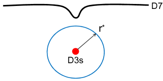
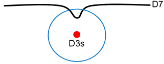
Fig. 1: Two typical D7 brane embeddings in the bulk space-time corresponding to a supersymmetric confining theory. The left and right hand figures show the insulator and the conductor phase respectively. The radius $r^{*}$ is explained in the text.

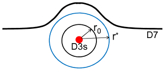
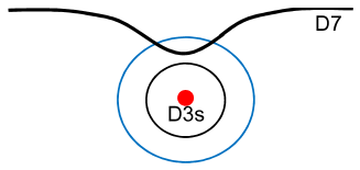
Fig. 2: The D7 embeddings for non-supersymmetric confining theory are shown. The left (right) shows insulator (conductor) phase. In this case, singularity exists and its position is shown by the radius $r_{0}$.

Other than the insulator-conductor transition, we find two new phase transitions in the confining theories. One is found in the insulator phase of the confining theory with chiral and super symmetries. For a fixed $E(<E_{\rm cr})$, we find a jump of the chiral condensate and also of the meson mass for light quarks $m_{q}(<m_{q}^{\rm cr})$, where $m_{q}^{\rm cr}$ varies with $E$ and we show a phase diagram in $m_{q}$-$E$ plane. We will see that the phase is due to the confining configuration. Another is the chiral phase transition in the confining theory with broken chiral and super symmetries. We find the vanishing of the chiral condensate for the massless quark at the insulator-conductor transition point. This implies the restoration of the chiral symmetry for $E>E_{\rm cr}$,

The pictures of D7 brane embeddings are shown for the two confining theories in the Figs. 1 and 2. In the Fig. 1, supersymmetric case is shown, and the non-supersymmetric one is given in the Fig. 2. The left hand figures of them show the insulator phase, and the chiral symmetry is preserved (broken) in the case of Fig.1 (Fig. 2). In the conductor phase, shown by the right hand figures, the chiral symmetry is preserved in both cases.

In section 2, we give the setting of our model for the supersymmetric and non-supersymmetric version of confining Yang-Mills theory. And the response to the electric field is studied in the following sections 3 and 4 for the supersymmetric case. For non-supersymmetric case, the analysis including the chiral transition are given in the section 5. and the summary is given in the final section.

2 D3/D7 model for confining YM theory

We start from 10d IIB model retaining the dilaton $\Phi$, axion $\chi$ and self-dual five form field strength $F_{(5)}$. Under the Freund-Rubin ansatz for $F_{(5)}$, $F_{\mu_{1}\cdots\mu_{5}}=-\sqrt{\Lambda}/2~{}\epsilon_{\mu_{1}\cdots\mu_{5}}$ [24, 25], and for the 10d metric as $M_{5}\times S^{5}$ or $ds^{2}=g_{MN}dx^{M}dx^{N}+g_{ij}dx^{i}dx^{j}$, we find the solution. The five dimensional $M_{5}$ part of the solution is obtained by solving the following reduced 5d action,

$$S={1\over 2\kappa^{2}}\int d^{5}x\sqrt{-g}\left(R+3\Lambda-{1\over 2}(\partial\Phi)^{2}+{1\over 2}e^{2\Phi}(\partial\chi)^{2}\right),$$ (1)

which is written in the string frame and taking $\alpha^{\prime}=g_{s}=1$.

The solution is obtained under the ansatz,

$$\chi=-e^{-\Phi}+\chi_{0}\ ,$$ (2)

which is necessary to obtain supersymmetric solutions. And the solution is expressed as

$$ds^{2}_{10}=G_{MN}dX^{M}dX^{N}~{}~{}~{}~{}~{}~{}~{}~{}~{}~{}~{}~{}~{}~{}\qquad$$

$$=e^{\Phi/2}\left\{{r^{2}\over R^{2}}A^{2}(r)\left(-dt^{2}+(dx^{i})^{2}\right)+\frac{R^{2}}{r^{2}}dr^{2}+R^{2}d\Omega_{5}^{2}\right\}\ .$$ (3)

Then, the supersymmetric solution is obtained as

$$e^{\Phi}=1+\frac{q}{r^{4}}\ ,\quad A=1\,,$$ (4)

where $M,~{}N=0\sim 9$ and $R=\sqrt{\Lambda}/2=(4\pi N)^{1/4}$. And $q$ represents the vacuum expectation value (VEV) of gauge fields condensate [10]. In this configuration, the four dimensional boundary represents the $\cal{N}$=2 SYM theory. In this model, we find quark confinement in the sense that we find a linear rising potential between quark and anti-quark with the tension $\sqrt{q}/R^{2}$ [24, 10].

As for the non-supersymmetric case, the solution is given by (3) and

$$A(r)=\left((1-(\frac{r_{0}}{r})^{8})\right)^{1/4},\qquad e^{\Phi}=\left(\frac{(r/r_{0})^{4}+1}{(r/r_{0})^{4}-1}\right)^{\sqrt{3/2}},\qquad\chi=0\,.$$ (5)

This configuration has a singularity at the horizon $r=r_{0}$. So we can not extend our analysis to near this horizon where higher curvature contributions are important. This theory provides confinement and chiral symmetry breaking. The latter means that we find non-zero chiral condensate for the massless quark. In other words, a dynamical quark mass would be generated for a massless quark in this theory. This point is different from the above supersymmetric background solution. The confinement is sustained by the gauge condensate, which is proportional to $r_{0}^{4}$ in the present case , as in the supersymmetric case.

3 D7 brane embedding and phase transitions

The D7 brane is embedded in the above background (3) as follows. First, the extra six dimensional part of the above metric (3) is rewritten as,

$$\frac{R^{2}}{r^{2}}dr^{2}+R^{2}d\Omega_{5}^{2}=\frac{R^{2}}{r^{2}}\left(d\rho^{2}+\rho^{2}d\Omega_{3}^{2}+(dX^{8})^{2}+(dX^{9})^{2}\right)\ ,$$ (6)

where $r^{2}=\rho^{2}+(X^{8})^{2}+(X^{9})^{2}$. And we obtain the induced metric for D7 brane,

$$ds^{2}_{8}=e^{\Phi/2}\left\{{r^{2}\over R^{2}}A^{2}\left(-dt^{2}+(dx^{i})^{2}\right)+\right.\qquad$$

$$\left.\frac{R^{2}}{r^{2}}\left((1+(\partial_{\rho}w)^{2})d\rho^{2}+\rho^{2}d\Omega_{3}^{2}\right)\right\}\ ,$$ (7)

where we set as $X^{8}=w(\rho)$ and $X^{9}=0$ without loss of generality due to the rotational invariance in $X^{8}$-$X^{9}$ plane. The embedded configuration is obtained as the solution for the profile function $w(\rho)$, and it is performed with non-trivial gauge field

$$A_{x}(\rho,t)=-Et+h(\rho)$$ (8)

in the D7 brane action. Here the chemical potential and the charge density are not introduced since we are considering in confinement phase where no free quark is allowed.

The brane action for the D7-probe is given as

$$S_{\rm D7}=-\tau_{7}\int d^{8}\xi\left(e^{-\Phi}\sqrt{-\det\left({\cal G}_{ab}+2\pi\alpha^{\prime}F_{ab}\right)}-{1\over 8!}\epsilon^{i_{1}\cdots i_{8}}A_{i_{1}\cdots i_{8}}\right)$$

$$+\frac{(2\pi\alpha^{\prime})^{2}}{2}\tau_{7}\int P[C^{(4)}]\wedge F\wedge F\ ,$$ (9)

where $F_{ab}=\partial_{a}A_{b}-\partial_{b}A_{a}$. ${\cal G}_{ab}=\partial_{\xi^{a}}X^{M}\partial_{\xi^{b}}X^{N}G_{MN}~{}(a,~{}b=0\sim 7)$ and $\tau_{7}=[(2\pi)^{7}g_{s}~{}\alpha^{\prime}~{}^{4}]^{-1}$ represent the induced metric and the tension of D7 brane respectively. And $P[C^{(4)}]$ denotes the pullback of a bulk four form potential,

$$C^{(4)}=\left(\frac{r^{4}}{R^{4}}dx^{0}\wedge dx^{1}\wedge dx^{2}\wedge dx^{3}\right)\ .$$ (10)

The eight form potential $A_{i_{1}\cdots i_{8}}$, which is the Hodge dual to the axion, couples to the D7 brane minimally. In terms of the Hodge dual field strength, $F_{(9)}=dA_{(8)}$ [26], the potential $A_{(8)}$ is obtained.

Then, by taking the canonical gauge, we arrive at the following D7 brane action,

$$S_{\rm D7}=-2\pi^{2}\tau_{7}~{}\int d^{4}xd{\rho}\rho^{3}\left({R\over r}e^{\Phi/2}\sqrt{Pe^{\Phi}-Q}-{q\over r^{4}}\right)\ ,$$ (11)

$$P=|\tilde{G}_{00}|\tilde{G}_{xx}\tilde{G}_{\rho\rho}\,,\quad Q=\tilde{G}_{\rho\rho}{\dot{\tilde{A}}_{x}}^{2}-|\tilde{G}_{00}|{{\tilde{A^{\prime}}}_{x}}^{2}$$ (12)

where $\tilde{G}_{MN}=e^{-\Phi/2}{G}_{MN}$, $\tilde{A}_{x}=2\pi\alpha^{\prime}{A}_{x}$ and the eight form part is given as $C_{8}(r)={q/r^{4}}$ [27]. The explicit forms of $\tilde{G}_{MN}$ are given as follows,

$$|\tilde{G}_{00}|=\tilde{G}_{xx}=\left({r\over R}\right)^{2}\,,\quad\tilde{G}_{\rho\rho}=\left({R\over r}\right)^{2}(1+w^{\prime}(\rho)^{2}).$$ (13)

At first, we solve the equation of motion of ${\tilde{A^{\prime}}}_{x}=\tilde{h^{\prime}}$ as

$$e^{\Phi/2}{\rho^{3}\over r}{|\tilde{G}_{00}|\tilde{A^{\prime}}_{x}\over\sqrt{Pe^{\Phi}-Q}}=B$$ (14)

where $B$ denotes a constant and it corresponds to the electric current,

$$\langle J_{x}\rangle=B\,.$$ (15)

Then we rewrite the D7 action by eliminating $\tilde{A^{\prime}}_{x}$ through the Legendre transformation,

$$U\equiv S-\int d^{4}xd\rho\tilde{A^{\prime}}_{x}{\delta S\over\delta\tilde{A^{\prime}}_{x}}$$ (16)

and we obtain

$$U=-2\pi^{2}\tau_{7}~{}\int d^{4}xd{\rho}L$$ (17)

$$L=\sqrt{{\tilde{G}_{\rho\rho}\over|\tilde{G}_{00}|}}\left\{\left(e^{\Phi}|\tilde{G}_{00}|\tilde{G}_{xx}-\tilde{E}^{2}\right)\left({\rho^{6}\over r^{2}}e^{\Phi}|\tilde{G}_{00}|-B^{2}\right)\right\}^{1/2}-{q\over r^{4}}{\rho^{3}\over R}$$ (18)

Explicit expression of $L$ in the present case is given as follows,

$$L=\left({R\over r}\right)^{2}\sqrt{1+{w^{\prime}}^{2}}\sqrt{\left({q+r^{4}\over R^{4}}-\tilde{E}^{2}\right)\left({\rho^{6}\over R^{2}}e^{\Phi}-B^{2}\right)}-{q\over r^{4}}{\rho^{3}\over R}$$ (19)

Then in our case, the locus vanishing point, where the insulator and conducting phase is separated, is given as

$${r^{*}}^{2}={\rho^{*}}^{2}+w^{2}(\rho^{*})=\sqrt{\tilde{E}^{2}R^{4}-q}$$ (20)

which is shifted by $q$. In other words, there is a threshold of $\tilde{E}$ at $q^{1/2}/R^{2}$ to generate a locus or the conducting area. Namely, for $\tilde{E}<q^{1/2}/R^{2}$, the electric current $B$ should be zero.

The equation of motion of $w(\rho)$ is obtained from the above $L$ as follows,

$$\partial_{\rho}\left({w^{\prime}\over\sqrt{1+{w^{\prime}}^{2}}}\sqrt{F(r)}\right)-{w\over r}\left({F^{\prime}(r)\over 2\sqrt{F(r)}}\sqrt{1+{w^{\prime}}^{2}}+{4q\rho^{3}\over r^{5}}\right)=0\,,$$ (21)

$$F(r)={\rho^{6}}e^{2\Phi}\left(1-{R^{4}\tilde{E}^{2}\over r^{4}e^{\Phi}}\right)\left(1-{R^{2}B^{2}\over\rho^{6}e^{\Phi}}\right)\,,$$ (22)

where $F^{\prime}(r)=\partial_{r}F(r)$.

3.1 Insulator Phase

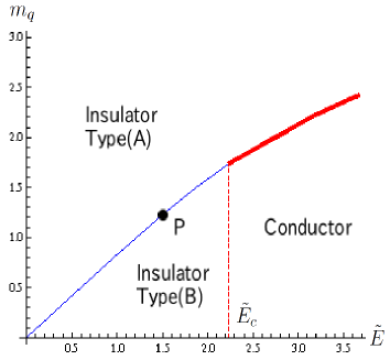
Fig. 3: The phase diagram in the $m_{q}$-$\tilde{E}$ space at $q=5$ and $R=1$. The thick solid (red) curve and the dashed (red) vertical line ($\tilde{E_{c}}=\sqrt{q}/R^{2}$) represent critical points between the insulator phase and the conductor phase. The thin solid (blue) curve represents the critical points between type (A) and type (B) phases in the same insulator phase. The point P corresponds to a transition point, and the jump of $c$ on this point is shown in the Fig. 4.

Here we concentrate on the insulator phase, where the electric field is restricted as

$${q\over R^{4}}\geq\tilde{E}^{2}\,.$$ (23)

In this case, we find $\left({q+r^{4}\over R^{4}}-\tilde{E}^{2}\right)>0$ for any $r$, then we could set $B=0$ or $\langle J_{x}\rangle=0$ in order to keep $F(r)$ to be positive. Then in this phase, the electric current is zero and we can call this case as insulator (see Fig. 3). The inequality (23) implies that the repulsive force between the quark and anti-quark due to the electric field is smaller than the attractive color force to confine them. For $q\neq 0$, we find the tension between the quark and anti-quark is equal to $q^{1/2}/R^{2}$ [10]. Thus, we can understand the above statement.

Under this setting, we solve the equation (21) and we could find two phases, type (A) and (B), which are shown in the phase diagram of the Fig. 3. The asymptotic form of the solution at $\rho\to\infty$ is obtained as

$$w(\rho)=m_{q}+\frac{c}{\rho^{2}}+\cdots\,,$$ (24)

where $m_{q}$ and $c=\langle\bar{\psi}\psi\rangle$ corresponds to the quark mass and the chiral condensate respectively. This correspondence is well known from the AdS/CFT dictionary. These quantities are fixed after solving (21) in all region of $\rho$ including the infrared region of $\rho=0$. The value of $c$ for any solution depends on $m_{q}$, $q$ and also $E$.

For $q=0$, the background is reduced to the supersymmetric AdS${}_{5}\times S^{5}$ and we find $c=0$ when $E=0$. When $E$ is turned on, we find the solution of negative $c$, which depends on the quark mass $m_{q}$ and decreases with decreasing $m_{q}$ monotonically. This case has been studied in [14].

Here we concentrate on the case of $q>0$, and the $m_{q}$ dependence of $c$ has been studied. For the case of $\tilde{E}=1.5$, $q=5$ and $R=1$, the D7 embedded solutions and the value of $c$ for various $m_{q}$ are shown in the Fig. 4 as a typical example. This analysis has been performed across the point $P$ in the Fig. 3. From the Fig. 4, a phase transition is observed through a jump of $c$ at $m_{q}=m_{q}^{\rm cr}\simeq 1.23$. This transition point depends on other parameters of the theory, especially sensitive to $E$. In the Fig 3, the line of this phase transition is shown in the $m_{q}-E$ plane. Each phase is assigned as (A) and (B) in the Fig. 3.

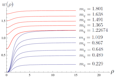
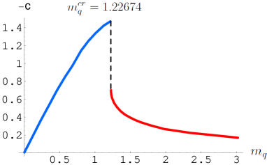
Fig. 4: Solutions $w(\rho)$ and $c$ for the various $m_{q}$ at $\tilde{E}=1.5$, $q=5$ and $R=1$. The left figure shows that solutions become almost zero at the $\rho=0$ for $m_{q}<m_{q}^{cr}(=1.22674)$, on the other hand, solutions are always finite for $m_{q}>m_{q}^{cr}$. The right figure shows that the chiral condensates $c$ jump at $m_{q}^{cr}$.

The jump of $c$ is explicitly reflected to the jump of the infrared end point of the solution, $w(0)$, which changes from a finite value to the very small value (almost zero) for the small quark mass, namely in the region $0\leq m_{q}\leq m_{q}^{\rm cr}$. On the other hand, it is known that the meson mass is proportional to $w(0)$ in the supersymmetric case of $E=0$, and we could see that this relation is retained even if $E>0$. Namely, after this transition for small $m_{q}$, the meson mass of $m_{q}\leq m_{q}^{\rm cr}$ also jumps from a finite value to almost zero.

Finally we give a comment about the similarity of the role of electric field $E$ to the temperature. The dynamical situation observed here is very similar to the case of the high temperature phase. The temperature gives thermal screening to the system of confining quarks to suppress the color force. The electric field $E$, on the other hand, pulls the quark and anti-quark to the opposite direction to compete the attractive confining force between the quark and anti-quark. In both cases, the confining force is effectively suppressed. In this sense, the role of $E$ is similar the temperature. As a result of this effect, $E$ pulls down the end point of D7 toward $r=0$, the horizon of the background metric. Our model gives quark confinement for $E=0$ due to the parameter $q$ [10], and the confining force is still stronger than the repulsion of $E$ in the phase (B). However we could find the conducting phase for $\tilde{E}\geq\sqrt{q}/R^{2}$ where the confinement force is defeated by the repulsion due to $E$ as shown below.

3.2 Meson spectrum

Here we consider meson spectrum in the insulator phase to understand well the phase transition observed in the previous section. The meson masses are given by solving the equations of motion of fluctuations of the fields on the D7 brane. The simplest and non-trivial one are the fluctuations of the gauge fields which are perpendicular to $(t,x,\rho)$ directions. They do not mix with the other fluctuations and are denoted by $A_{\bot}$. We impose the following ansatz for $A_{\bot}$,

$$\delta A_{2,3}=\delta A_{\bot}=e^{-i(\omega t-k_{x}x)}A_{\bot}(\rho)\,,$$ (25)

where we consider the $y,z$ components of $\delta A_{\bot}=\delta A_{y,z}$ for the simplicity. Then, the action is expanded up to the quadratic part about $\epsilon$,

$$S_{D7} = \tau_{7}\int d^{8}\xi L_{0}\left(1+\tilde{L}^{(2)}_{A_{\bot}}+\cdots\right)\,,$$

$$L^{(2)}_{A_{\bot}} {\equiv} L_{0}\tilde{L}^{(2)}_{A_{\bot}}={1\over 2}L_{0}\tilde{G}^{ab}\tilde{G}^{\bot\bot}\partial_{a}\delta A_{\bot}\partial_{b}\delta A_{\bot}\,,$$ (26)

where

$$\tilde{G}^{\rho\rho} = \left({r^{4}\over R^{4}}-\tilde{E}^{2}e^{-\Phi}\right)/G_{(3)}\,,$$ (27)

$$\tilde{G}^{\rho t} = -{{B}\tilde{E}R^{2}\over\rho^{3}re^{\Phi}\sqrt{G_{(3)}}}\,,$$ (28)

$$\tilde{G}^{tt} = -\left(1+{w^{\prime}}^{2}+{B}^{2}{G_{(3)}R^{4}\over\rho^{6}r^{2}e^{\Phi}}\right)/G_{(3)}\,,$$ (29)

$$\tilde{G}^{\bot\bot} = \left({r\over R}\right)^{2}\,,$$ (30)

$$G_{(3)} = {r^{2}\rho^{6}\over R^{4}}(1+w^{\prime}(\rho)^{2}){1-\frac{R^{4}\tilde{E}^{2}}{r^{4}e^{\Phi}}\over{\rho^{6}/R^{2}}-{{B}^{2}e^{-\Phi}}}\,,$$ (31)

$$L_{0}={\rho^{6}\over R}\sqrt{(1+w^{\prime}(\rho)^{2})}\sqrt{\left(1-\frac{R^{4}\tilde{E}^{2}}{e^{\Phi}r^{4}}\right)/\left({\rho^{6}\over R^{2}}-\frac{B^{2}}{e^{\Phi}}\right)}\,.$$ (32)

In the case of the insulator phase, we set as $B=0$, then we obtain

$$L^{(2)}_{A_{\bot}}=e^{-2i(\omega t-k_{x}x)}\rho^{3}~{}\frac{-\frac{R^{4}}{r^{4}}(1+w^{\prime}(\rho)^{2})M^{2}A_{\bot}^{2}(\rho)+\left(1-\frac{R^{4}\tilde{E}^{2}}{e^{\Phi}r^{4}}\right){A^{\prime}}_{\bot}^{2}(\rho)}{\sqrt{(1+w^{\prime}(\rho)^{2})\left(1-\frac{R^{4}\tilde{E}^{2}}{e^{\Phi}r^{4}}\right)}}\,,$$ (33)

where prime denotes the derivative with respect to $\rho$ and $M^{2}=-k^{2}=-\omega^{2}+k_{x}^{2}$, which defines the mass of the mesons. Then the equation of motion of $A_{\bot}(\rho)$ is obtained as follows,

$$A^{\prime\prime}_{\bot}(\rho)+\left({3\over\rho}+{H^{\prime}\over H}\right)A^{\prime}_{\bot}(\rho)+\frac{R^{4}M^{2}}{r^{4}H^{2}(\rho)}A_{\bot}(\rho)=0,$$ (34)

$$H(\rho)=\sqrt{\frac{1-\frac{R^{4}\tilde{E}^{2}}{e^{\Phi}r^{4}}}{1+w^{\prime}(\rho)^{2}}}\ .$$ (35)

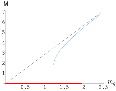
Fig. 5: The lightest meson mass for $\tilde{E}=1.5$, $q=5$ and $R=1$. The (blue) solid curve shows the meson mass of Minkowski embedding solutions. The (red) horizontal line shows (almost) massless mesons of the solution of embedding at the origin at the end point. The dashed line represents the lightest meson for $\tilde{E}=0$ given by (41) since $m_{q}=w(0)$. For $m_{q}<m_{cr}=1.22674$, all meson masses are almost zero.

Here we notice the following two points. Firstly, the mass eigenfunction should be normalizable with respect to $\rho$ integration in (3.2), then we impose the following boundary condition,

$$\int^{\infty}d\rho L^{(2)}_{A_{\bot}}<\infty\,.$$ (36)

Then we find the following condition for the asymptotic behavior of $A_{\bot}(\rho)$ at large $\rho$,

$$A_{\bot}(\rho)|_{\rho\to\infty}\to O(\rho^{-\beta})\to 0\,,\quad\beta>1\,.$$ (37)

This condition leads to discrete meson mass spectrum.

Secondly, consider the infrared limit ($\rho=0$) for the equation (34). Assuming the leading term of $A_{\bot}$ in this region as

$$A_{\bot}(\rho)|_{\rho\to 0}\simeq\rho^{\alpha}\,.$$ (38)

Then, the asymptotic form of the equation is considered by separating to the two cases.

(i) For $w(0)\neq 0(>0)$, we find from (34) the following form,

$$\alpha(\alpha+2)\rho^{\alpha-2}+\frac{R^{4}M^{2}}{w(0)^{4}H^{2}(0)}\rho^{\alpha}+\cdots=0$$ (39)

where $\cdots$ denotes the terms of higher order of $\rho$.

(ii) For $w(0)=0$, we have

$$\frac{R^{4}M^{2}}{H^{2}(0)}\rho^{\alpha-4}+\alpha(\alpha+2)\rho^{\alpha-2}+\cdots=0\,.$$ (40)

For the first case, (i) $w(0)\neq 0$, we find $\alpha=0$ or $-2$ from (39). And we find finally $\alpha=0$ from the normalizability of $A_{\bot}(\rho)$. Then, finite mass eigenvalues of $M$ are found by these boundary conditions in this case.

As for the second case of $w(0)=0$, we must take $M=0$ and $\alpha=0$. This implies that all the meson mass of the bound state of quark and anti-quark with $m_{q}\leq m_{q}^{\rm cr}$ should be zero.

This is consistent with the meson spectra obtained for $\tilde{E}=0$ [4],

$$M=2\sqrt{n(n+1)}\frac{w(0)}{R^{4}}\,,\quad n=1,2,\cdots.$$ (41)

And also at finite $E$, we find approximately this formula for the meson spectrum. The numerical results are shown in the Fig. 5 for $\tilde{E}=1.5$ and $q=5$. This result supports our statement given above.

As for the exact value of $w(0)$ in this case, it is difficult to say that it is zero or finite but small since there is no analytical support of this statement. So, we can say only that the meson mass is very small in the phase (B).

4 Insulator-Conductor transition

Here we consider the large $E$ which satisfies the following inequality,

$$\tilde{E}^{2}>{q\over R^{4}}\,.$$ (42)

In this case, there is a position of $r$ called as a locus vanishing point defined as

$$r^{*}=\left(R^{4}\tilde{E}^{2}-q\right)^{1/4}\,,$$ (43)

where the action vanishes. Then we need non-zero $B$ in order to preserve the reality of the action even in the region of $r<r^{*}$ [12]. This guarantees the existence of the solution $w(\rho)$ up to the region, $w^{2}(\rho)<{r^{*}}^{2}-\rho^{2}$, since the equation of motion of $w$ must be also real. Then, for these solutions, $w$, the electric current $B$ must be accompanied in spite of the fact that the theory is in the quark confinement phase, where we can not introduce charge density $n_{b}$ as mentioned above.

Carrier of the current $B$:

Up to now, this phenomenon has been considered in the non-confining high temperature phase, and the carrier of this current can be identified with the quark and the anti-quark which are pair created by the strong electric filed [12]. And, the configuration of the quark or the anti-quark is given by the string connecting the probe brane and the event horizon, which exists in the holographic high temperature model.

In our confining theory, however such a quark string configuration can not be considered since the event horizon does not exist. One may therefore wonder what is the carrier of this baryon number current, $B$, in the present confining case.

One possibility might be the pair created baryons and anti-baryons which are allowed in the confinement phase as considered in the type IIA model [22]. Another possibility is to consider the creation of mesons which have opposite charge. But the latter case would be meaningful only for some flavor non-singlet current as discussed in [18]. In the present case, however, we restrict our attention to the $U(1)_{B}$ current, so we don’t consider this case.

The first possibility does not contradict with the present model. But, in our model, the current appears when the electric force ($\tilde{E}$) for a unit quark number exceeds the confinement attractive force, which is given by the tension, $q^{1/2}/R^{2}$, of linear rising potential between the quark and the anti-quark to bind them [10]. Therefore, we are led to the idea that the main part of the current should be reduced to the pair created quark and anti-quark, which can not be bound to mesons since the attractive force is suppressed by the strong electric repulsion.

Meanwhile, we must remind that the theory considered here describes the confining phase. Then, it seems to be controversial to suppose the quark and the anti-quark as the current carrier. In spite of this fact, as explained below, it would be natural to consider such that the carriers of the current $B$ would be the quarks and the anti-quarks. One reason is that the mesons would be melt down into quarks and anti-quarks for the solutions ($w$) with finite $B$ as shown in the next subsection for the case of quarks with small-mass compared to the given $\tilde{E}$.

However we should notice that the melted mesons may not be changed to the string state of quarks as seen in the high temperature deconfinement phase. The reason is that the dual gravitational geometry of the confining gauge theories given here has no event horizon, which could be the end point of the free quark-string configuration. As the resolution of this problem, we point out two possibilities.

One possible way is to consider the interaction between the bulk and the probe D7 branes, in which the electric field is imposed. This is equivalent to include $1/N_{c}$ corrections to the theory. We expect that this correction deforms the bulk solution to the type of AdS-Schwartzschild solution which has a horizon. This implies that the system get a low temperature as a result. Then, we can suppose the configuration of the quark string connecting the D7 brane and the horizon. But we do not perform this analysis here and it is remained as a future work.

The second idea of the resolution is as follows. In the conductor phase of the present theory, the quark and the anti-quark are living in the unstable “mesons”, which are called as the quasi-normal state given in the next sub-section, and are supposed to be accelerated in the opposite direction. Such a string configuration is still expressed by the U-shaped one, and the both end points are on the D7 brane. A time-dependent configuration, which would correspond to this string-configuration, has been found as an exact classical solution of the equation of motion of the fundamental string in the AdS₅ space time [23].

This configuration is separated to three parts by dividing it at a special points of the radial coordinate $(r=r_{b})$ in AdS₅. The upper two parts for $r>r_{b}$ correspond to the quark and the anti-quark, which are moving with the velocity below the speed of light. The speed of the lower part however exceeds the speed of the light. Then the causal parts of the quark and the anti-quark strings end at $r_{b}$. The observer on the boundary could see the disconnected quark and anti-quark, which lose its energy into the lower part as the radiation of the accelerated charged particle [23]. This movement of the quark and anti-quark would be related to the current $B$.

This situation is very similar to the high temperature case, where the causal parts of the quark and the anti-quark end at the horizon. It would be possible to find a similar configuration also in the confining bulk background.

While the configuration of this state is an U-shaped string whose end points are on the probe brane, this can be changed to a static string with the Rindler temperature by an appropriate coordinate transformation [23]. Then the accelerated configuration mentioned above would be considered as an equivalent configuration given at finite temperature within a coordinate transformation.

In the case of high temperature, deconfinement phase, we find the same quasi-normal mode for the mesons in the conductor phase. Then it would be possible to see the same carrier of the current $B$ also in the deconfinement theory. However, there is an event horizon in this case at $r_{H}$, so we could not see the same carrier mentioned above when $r_{H}$ is larger than $r_{b}$. It would be an interesting problem to study this point, but it is postponed as a future work here.

Numerical solutions:

In the next, we show the numerical solutions in the conducting phase. In solving numerically the equation of motion(21), we impose the boundary condition at the locus point as follows because of continuity of the solution $w(\rho)$,

$$\lim_{\epsilon\to 0}w(\rho_{*}-\epsilon)_{\rm in}=\lim_{\epsilon\to 0}w(\rho_{*}+\epsilon)_{\rm out},\ \ \ \ \lim_{\epsilon\to 0}w^{\prime}(\rho_{*}-\epsilon)_{\rm in}=\lim_{\epsilon\to 0}w^{\prime}(\rho_{*}+\epsilon)_{\rm out},$$ (44)

where $w(\rho_{*})_{\rm in(out)}$ represents the value slightly inside (outside) of the locus vanishing point.

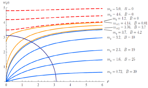
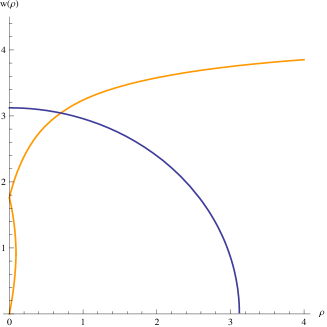
Fig. 6: The solutions $w(\rho)$ for $\tilde{E}>q^{1/2}/R^{2}$. Here we plot them for $\tilde{E}=10$, $q=5$ and $R=1$. Left: The upper dashed (red) curves represent the one of insulator phase and they do not pass the locus vanishing point shown as a quarter of a circle. There are two types of solutions of the conductor phase. The middle (orange) ones end at finite $w(0)$. On the other hand, the lower (blue) ones end at $w(0)=0$. Right: The actual conical singular solution of D7-brane. The conical singular solutions actually reflects at finite $w(0)$ and intersects to the event horizon $\rho=0$.

The typical example of the numerical results are shown in the Fig. 6. In general, the solutions are separated to three groups. (i) For large quark mass, the solution does not need $B$ since it does not cross the locus vanishing point. So the quarks are still in the insulator phase.

When the quark mass decreases, the second group solutions are obtained. The solutions $w(\rho)$ reach at the locus point, and these solutions demand finite $B$. In spite of the fact that the theory is in the confinement phase, the carrier of this current can be considered as the quarks and anti-quarks as explained above.

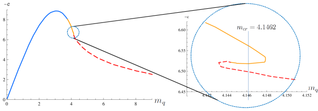
Fig. 7: The relation between the chiral condensation $c$ and the quark mass at $\tilde{E}=10$, $q=5$ and $R=1$. The solid curve includes two types of solution ((ii) and (iii)), namely blue curve ((iii)) and orange one ((ii)). The dashed (Red) curve represents the solution in the insulator phase. We can see a first order phase transition between insulator phase and conductor phase (from (i) to (ii)) from the right figure, where microscopic analysis is given. The critical mass $m_{cr}$ for this phase transition is estimated by using the equal-area law.

Moreover, we find the solutions in the conducting phase are separated to two types (see Fig.6). (ii) One satisfies $w(\rho=0)\neq 0$, and these solutions have a conical singularity. (iii) Another satisfies $w(\rho=0)\simeq 0$, which seems smoothly reaching at the origin without any singular behaviour.

The conical singular solution seems to be ending at finite $w(0)$ before reaching to the origin (here $r=0$), namely the event horizon. The solution which passes through $r^{*}$ must have the electric current $B$ with its charge carriers, so the brane must end at the horizon. Actually, we could find that the D7-brane of the category (ii) (classified as conical singular solution) could eventually reach to the horizon as shown in the right hand side of the Fig. 6. This result is consistent with the result obtained in the deconfining case [15, 30].

We don’t have any reasonable physical interpretation for the solutions of category (ii) from the gauge theory side. One possible resolution for this singular solution is that we would need some stringy corrections to remove this kind of solutions and to obtain more smooth solutions, especially in the region of inside the locus vanishing point $r<r^{*}$. For the region $r>r^{*}$, we consider however that such corrections would be negligible and we could find physical insight.

In order to see the property of the transitions of these three types of solutions, we studied the relation between quark mass $m_{q}$ and the VEV of quark bilinear $c=\langle\bar{\psi}\psi\rangle$, and the numerical results are shown in the Fig. 7. For the transition from insulator to the conductor (from (i) to (ii)), the result shows the multi-valuedness of $c$ as a function of $m_{q}$ near the transition point. This implies the typical behavior of the first-order phase transition. On the other hand, for the transition from $w(0)\neq 0$ to $w(0)=0$ (from (ii) to (iii)), we could not find any jump of $c$.

4.1 Quasi-normal mode and meson melting

In the conductor phase, the solution $w(\rho)$ crosses the locus vanishing point. In this case, we can see that there is no stable meson state since the energy eigenvalue is complex. These are known as quasi-normal mode [28, 31, 32]. In the present confining theory, the same mode are found as shown below.

Here, we consider the meson spectrum in the conductor phase. For simplicity, we analyze the transverse components of the vector mesons, $\delta A_{\bot}=\delta A_{y,z}$ given in the previous section (3.2), by imposing the following form of fluctuations,

$$\delta A_{\bot}=e^{-i\omega t}\xi(\rho).$$ (45)

Then, the equation of motion of $\xi(\rho)$ is obtained:

$${\cal G}^{\rho\rho}\xi^{\prime\prime}(\rho)+\left(\partial_{\rho}{\cal G}^{\rho\rho}-2i\omega{\cal G}^{\rho t}\right)\xi^{\prime}(\rho)+\left(-\omega^{2}{\cal G}^{tt}-i\omega\partial_{\rho}{\cal G}^{\rho t}\right)\xi(\rho)=0,$$ (46)

where

$${\cal G}^{\rho\rho} = L_{0}{R^{2}\over r^{2}}\tilde{G}^{\rho\rho}\,$$ (47)

$${\cal G}^{\rho t} = {\cal G}^{t\rho}=2L_{0}{R^{2}\over r^{2}}\tilde{G}^{\rho t}\,$$ (48)

$${\cal G}^{tt} = L_{0}{R^{2}\over r^{2}}\tilde{G}^{tt}\,$$ (49)

Here $B$ is retained as non-zero value, and $\tilde{G}^{\rho\rho},\dots,\tilde{G}^{tt}$ are given in (27).

According to [28], one boundary is set at the locus vanishing point, $r=r^{*}$ and $\rho=\rho^{*}$, where

$${r^{*}}^{4}e^{\Phi(r^{*})}=R^{4}\tilde{E}^{2}\,,\quad{\rm and}\quad{\rho^{*}}^{6}e^{\Phi(r^{*})}=R^{2}B^{2}\,$$ (50)

are satisfied.

So the equation is firstly examined at this point. Near this point the factors in the equation (46) are expanded by the powers of $\epsilon\equiv\rho-\rho^{*}(<<1)$ as follows,

$${\cal G}^{\rho\rho} = a^{\rho\rho}_{1}\epsilon+O(\epsilon^{2})\,$$ (51)

$${\cal G}^{\rho t} = {\cal G}^{t\rho}=-a^{\rho t}_{0}+a^{\rho t}_{1}\epsilon+O(\epsilon)\,$$ (52)

$${\cal G}^{tt} = a^{tt}_{0}+O(\epsilon)\,,$$ (53)

where $(a^{\rho\rho}_{1},\dots)$ are calculable finite coefficients. The explicit form of these coefficients are abbreviated since they are complicated. We like to notice one point that $a^{\rho t}_{0}$ is positive. Then we find the leading part of the equation,

$$\xi^{\prime\prime}(\rho)+{1\over\epsilon}\left(1+2i\omega{a^{\rho t}_{0}\over a^{\rho\rho}_{1}}\right)\xi^{\prime}(\rho)+{1\over\epsilon}\left(-\omega^{2}{a^{tt}_{0}\over a^{\rho\rho}_{1}}-i\omega{a^{\rho t}_{1}\over a^{\rho\rho}_{1}}\right)\xi(\rho)=0,$$ (54)

From equation (54), the solution near $\rho=\rho^{*}$ is obtained as the linear combination of two independent series,

$$\xi=\alpha\epsilon^{-i\omega{a^{tt}_{0}\over a^{\rho\rho}_{1}}}\xi^{(1)}(\rho)+\beta\xi^{(2)}(\rho)$$ (55)

where $\alpha$ and $\beta$ are arbitrary constants, and $\xi^{(1)}(\rho)$ and $\xi^{(2)}(\rho)$ are expanded as

$$\xi^{(1,2)}(\rho)=a_{0}+a_{1}\epsilon+\cdots\,.$$ (56)

The first term of the solution (55) represents the incoming wave which should be meaningful in the present case[14]. So we consider the case of $\beta=0$.

As shown in the high temperature model[28, 31, 32], this incoming solution is connected to the local solution obtained at large $\rho$, where we find also two independent solutions. In order to connect the solutions in the large and small $\rho$ regions, the condition is taken such that the solution given above is smoothly connected to the normalizable one. This condition provides discrete values of $\omega$, which are complex, and the inverse of $\omega$ gives the decay constant of these modes. They are the quasi-normal modes mentioned above, and this implies that the mesons melt into the quark and anti-quark in the conductor phase.

In the present case, the role of the locus vanishing point seems to plays as an effective horizon, though the bulk configuration has no horizon and the locus vanishing point is made by the strong electric field. Therefore the dynamical role of the electric field is similar to the temperature. Then, we could propose the conical singularity does not effect the phase diagram in the previous section because the gauge theory could be ignorant of the physics inside of the locus vanishing point.

5 Non-Supersymmetric case and Chiral Transition

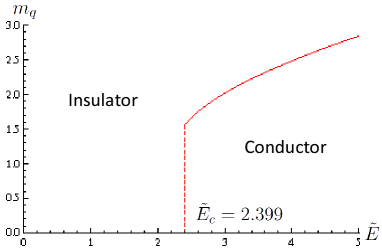
Fig. 8: The phase diagram for the non supersymmetric theory on the $m_{q}$-$\tilde{E}$ plane for $r_{0}=1$ and $R=1$. The solid curve and dashed line represents the critical points between the insulator phase and the conductor phase. The dashed line is estimated by the minimum of $T(r)$ (60).

Here we consider the solution given by (5). The electric field is added in a parallel way as given in the supersymmetric case. The D7 brane is embedded in the world volume (7), and the electric field is added by (8). Then, after the Legendre transformation, the D7 brane Lagrangian with the electric field is given as

$$L_{D7}=\sqrt{(1+w^{\prime}(\rho)^{2})F_{A}(r)}\,,$$ (57)

where

$$F_{A}(r)={\rho^{6}}e^{2\Phi}A^{8}\left(1-{R^{4}\tilde{E}^{2}\over r^{4}A^{4}e^{\Phi}}\right)\left(1-{R^{2}B^{2}\over\rho^{6}A^{6}e^{\Phi}}\right)\,.$$ (58)

Then the equation of motion of $w$ is obtained from the above $L_{D7}$ as follows,

$$\partial_{\rho}\left({w^{\prime}\over\sqrt{1+{w^{\prime}}^{2}}}\sqrt{F_{A}(r)}\right)-{w\over r}\sqrt{1+{w^{\prime}}^{2}}{F_{A}^{\prime}(r)\over 2\sqrt{F_{A}(r)}}=0\,,$$ (59)

where $F_{A}^{\prime}(r)=\partial_{r}F_{A}(r)$.

We solve this equation in two phases shown in the Fig. 8. The phase diagram is given in $m_{q}$-$E$ plane as in the case of the supersymmetric case. It is similar to the one shown in the Fig. 3 for the supersymmetric case, but we can not find two phases in the insulator side. This point is explained below.

5.1 Insulator phase

It is a little complicated to see the region of the insulator in the present case. From Eqs.(57) and (58), the insulator phase is restricted to the region

$$\tilde{E}R^{2}\leq A^{2}e^{\Phi/2}r^{2}\equiv T(r)$$ (60)

for any $r$. It is easy to see that $T(r)$ has a minimum in the region of $r>r_{0}$. To understanding its behavior, we show $T(r)$ for $r_{0}=1$ and $R=1$ in the Fig. 9.

As mentioned, we find the minimum of $T(r)$, and we determine the critical value of the electric field as $\tilde{E}\equiv\tilde{E}_{c}(=2.399)$ in terms of the inequality (60). This inequality is satisfied for $\tilde{E}\leq\tilde{E}_{c}$ at any $r$. Then, the conductor phase appears in this region.

Fig. 9: The solid (red) curve shows $T(r)\equiv A^{2}e^{\Phi/2}r^{2}$ at $r_{0}=1$ and $R=1$. The minimum of $T(r)$ is shown by the dotted line at $T=2.399(=\tilde{E}_{c})$. The locus vanishing point ($r^{*}$) for $\tilde{E}>\tilde{E}_{c}$ is obtained by the larger cross point between $T(r)$ (red curve) and the horizontal line at $T=\tilde{E}$ (solid blue line).

We solve the equation of $w$ for the case for $\tilde{E}=1.5$ (far below $\tilde{E}_{c}$) and $\tilde{E}=2.385$ (just below $\tilde{E}_{c}$) in this insulator region. The solutions at these points give typical behavior of the insulator solutions. The resultant solutions are shown in the Fig. 10 for various current quark masses, $0\leq m_{q}\leq 1.795$ for $\tilde{E}=1.5$ (the left figure) and $0\leq m_{q}\leq 2.319$ for $\tilde{E}=2.385$ (the right figure) respectively. For these parameters, the chiral condensate $c$s are shown for each $m_{q}$ in the Fig. 11.

In the supersymmetric case, the insulator phase has been separated to two phases (A) and (B) as shown in the Fig.3. The transition between (A) and (B) is observed by the jump of the chiral condensate $c$ at some $m_{q}$. However, as shown in the Fig. 11, there is no such jump in the present non-supersymmetric case. This is understood as follows. The end points $w(0)$ of each solutions for various small quark-mass at $\tilde{E}=1.5$ do not degenerate as shown in the case of the supersymmetric solutions, which are given in the Fig. 4. This implies that there is no critical point of $m_{q}$, where the value of the chiral condensate $c$ jumps.

As $\tilde{E}$ approaches to $\tilde{E}_{c}$, the value of $w(\rho=0)$ for small quark masses closes to each other. For $\tilde{E}=2.385$, which is just below of $\tilde{E}_{c}$, $w(\rho=0)$ for small quark mass seems to be almost degenerate as shown in the right of Fig.10, but we could not find the jump of $c$ as shown in the Fig. 11.

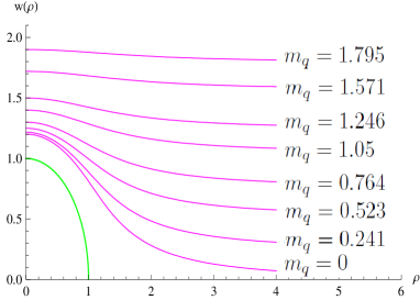
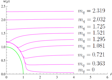
Fig. 10: The solution $w(\rho)$ for various $m_{q}$ at $\tilde{E}=1.5$ (left figure) and $\tilde{E}=2.385$ (the right figure) $r_{0}=1$, and $R=1$. The (green) circle represents the singularity at $r=r_{0}$.

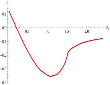
Fig. 11: The relation between quark mass $m_{q}$ and the VEV of quark bilinear $c=\langle\bar{\psi}\psi\rangle$ for $\tilde{E}=1.5$ (the left figure) and $\tilde{E}=2.385$ (the right figure) at $r_{0}=1$ and $R=1$.

5.2 Conductor phase

Now we turn to the conductor solutions. For $\tilde{E}\geq\tilde{E}_{c}$, there appears the locus vanishing point, $r=r^{*}$, which is determined for a fixed $\tilde{E}$ as

$$T(r^{*})=\tilde{E}\,.$$ (61)

We could find two such points from Fig 9, but here we define $r=r^{*}$ by the larger one. As for the smaller cross-point given by (61), we do not consider it since it exists very near to the singular point $r_{0}$, where the theory requires many more higher curvature terms. We like to discuss on this point in the future.

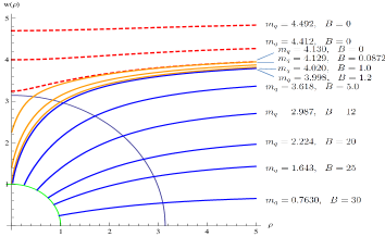
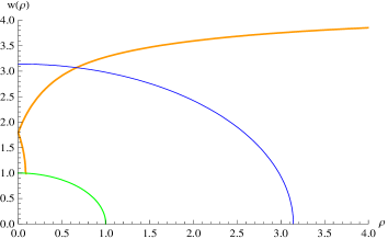
Fig. 12: Left figure:The solutions $w(\rho)$ are shown for $\tilde{E}=10(>\tilde{E}_{c})$, $r_{0}=1$ and $R=1$. The inner (green) and the outer (blue) circles represent the singular point $r=r_{0}$ and the locus vanishing point $r=r^{*}$ respectively. Right: The conical singular solution of D7-brane is shown in detail.

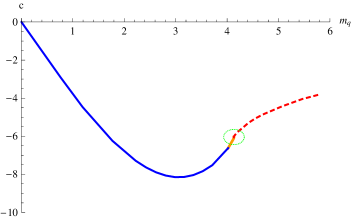
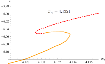
Fig. 13: The relation between condensation and the quark mass at $\tilde{E}=10$, $r_{0}=1$ and $R=1$. The solid (blue and orange) curves represent the solution in conductor phase. The orange curves represent the conical singular solutions. The dashed (red) curves represent the solution in the insulator phase. The critical mass $m_{c}=4.1321$ between conductor phase and insulator phase is estimated by using an equal-area law as shown in the right-hand figure.

For the conductor solutions, $B$ is determined as

$$B={\rho^{*}}^{3}A^{3}(r^{*})e^{\Phi(r^{*})/2}/R\,,$$ (62)

then $w(\rho)$ could enter into the region $r<r^{*}$ in this case. Thus we solve the equation of motion for $w(\rho)$ by imposing the same boundary condition (44) at the locus point as in the supersymmetric case.

In order to study the typical solution, we study the case of $\tilde{E}=10.0$, $r_{0}=1$ and $R=1$, and the results are shown in the Fig. 12. As expected, for large quark mass, we find the solutions of the insulator phase. They are shown by the upper (red) curves, which are above the locus vanishing point $r^{*}$. The middle (green) curves and the lower (blue) curves represent the solutions for the conductor phase. The middle (orange) solutions and the lower (blue) one represent the one for the conductor phase. The middle (orange) one are the conical singular solutions, and they are bounced once on the $w$-axis then going down to the singular circle $(r_{0})$ as shown in the right-hand figure of Fig 13. The lower (blue) solutions pass through the locus vanishing point and could approach smoothly to the point on the $r_{0}$.

In the next, we study the relation between quark mass $m_{q}$ and the VEV of quark bilinear $c=\langle\bar{\psi}\psi\rangle$ near the transition in order to see the property of the transition between different group of solutions. In the Fig. 13, we show the results obtained near the transition point between the insulator and the conductor. From this figure, we find the jump of $c$ at about $m_{q}\simeq 1.6$.

5.3 Chiral Transition

Here we concentrate on the chiral condensate $c=\langle\bar{\psi}\psi\rangle$ for the massless quark.

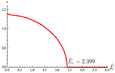
Fig. 14: The relation between the VEV of chiral condensate $c=\bar{\langle\psi}\psi\rangle$ and $\tilde{E}$ for massless quark at $r_{0}=1$, $R=1$. $c$ becomes zero for $\tilde{E}\geq\tilde{E}_{c}=2.399$

When $c=0$, we find chiral symmetry for the massless quark, but it is spontaneously broken when we obtain $c\neq 0$. In the present case, the chiral symmetry is broken at $E=0$. The results of our calculation are shown in the Fig. 14. For small $E$, we have finite $c$, then the chiral symmetry is spontaneously broken even if $E\neq 0$ in the present non-supersymmetric confining theory [10]. However, $c$ vanishes in the conducting phase of $\tilde{E}>\tilde{E}_{c}$ as shown in the Fig. 14.

Namely, the chiral symmetry is restored in the conducting phase where the confinement force has been overcome by the strong electric repulsion. In other words, the attractive force to generate finite VEV $c=\langle\bar{\psi}\psi\rangle$ has been eliminated by the electric field. Similar result has been shown in [37], where the analysis has been performed in terms of a special form of string operator based on the Sakai-Sugimoto model [38] considered in the type IIA theory. We notice here that the magnetic field has opposite role. Namely, it breaks the chiral symmetry of the symmetric theory as shown by various holographic method [17, 34, 35].

On the other hand, some analyses by the 4D field theories are also given in [36]. In that paper, the authors have studied the Nambu-Jona-Lasino model with constant electromagnetic field and shown that chiral symmetry is restored above a certain critical electric field strength. This result is consistent with our results. They have also shown the magnetic field breaks the chiral symmetry.

5.4 Meson melting and Quasi-normal mode

As the above supersymmetric case, the quarks are confined also in the present case, then we think the charge carriers as the quark and anti-quark which are in a special state discussed in the supersymmetric case. Namely the carriers are formed of the melted mesons due to the strong electric field.

Here, we consider the meson spectrum in the conductor phase as in the supersymmetric case. We analyze the vector mesons, $\delta A_{\bot}^{\rm NS}=\delta A_{y,z}^{\rm NS}$, where the notation ”NS” is used to discriminate it from the supersymmetric case. Then we express the fluctuations in the similar form to the supersymmetric case,

$$\delta A_{\bot}^{\rm NS}=e^{-i\omega t}\xi_{\rm NS}(\rho).$$ (63)

And, the equation of motion of $\xi_{\rm NS}(\rho)$ is obtained:

$${\cal G}^{\rho\rho}_{\rm NS}\xi^{\prime\prime}_{\rm NS}(\rho)+\left(\partial_{\rho}{\cal G}^{\rho\rho}_{\rm NS}-2i\omega{\cal G}^{\rho t}_{\rm NS}\right)\xi^{\prime}_{\rm NS}(\rho)+\left(-\omega^{2}{\cal G}^{tt}_{\rm NS}-i\omega\partial_{\rho}{\cal G}^{\rho t}_{\rm NS}\right)\xi_{\rm NS}(\rho)=0,$$ (64)

where

$${\cal G}^{\rho\rho}_{\rm NS} = L_{0}^{\rm NS}{R^{2}\over r^{2}A^{2}}\tilde{G}^{\rho\rho}_{\rm NS}\,$$ (65)

$${\cal G}^{\rho t}_{\rm NS} = {\cal G}^{t\rho}_{\rm NS}=2L_{0}^{\rm NS}{R^{2}\over r^{2}A^{2}}\tilde{G}^{\rho t}_{\rm NS}\,$$ (66)

$${\cal G}^{tt}_{\rm NS} = L_{0}^{\rm NS}{R^{2}\over r^{2}A^{2}}\tilde{G}^{tt}_{\rm NS}\,$$ (67)

where

$$L_{0}^{\rm NS} = A^{2}{R\over r}\rho^{3}\sqrt{G_{(3)}^{\rm NS}}\,$$ (68)

$$\tilde{G}^{\rho\rho}_{\rm NS} = \left(A^{4}{r^{4}\over R^{4}}-\tilde{E}^{2}e^{-\Phi}\right)/G_{(3)}^{\rm NS}\,$$ (69)

$$\tilde{G}^{\rho t}_{\rm NS} = -{{B}\tilde{E}R^{2}\over\rho^{3}rA^{6}e^{\Phi}\sqrt{G_{(3)}^{\rm NS}}}\,$$ (70)

$$\tilde{G}^{tt}_{\rm NS} = -A^{2}\left(1+{w^{\prime}}^{2}+{B}^{2}{G_{(3)}R^{4}\over A^{14}\rho^{6}r^{2}e^{\Phi}}\right)/G_{(3)}^{\rm NS}\,$$ (71)

$$G_{(3)}^{\rm NS} = {r^{2}A^{4}\over R^{2}}(1+w^{\prime}(\rho)^{2}){1-\frac{R^{4}\tilde{E}^{2}}{r^{4}A^{4}e^{\Phi}}\over{1-{{B}^{2}R^{2}\over\rho^{6}A^{6}e^{-\Phi}}}}$$ (72)

These are different from the supersymmetric case by the factor $A(r)$ and the form of the dilaton $e^{\Phi}$. In the present case, then, the locus vanishing point $\rho^{*}$ is determined by (61). The point is slightly shifted compared to the supersymmetric case. However, we should notice that $A(r)$ is not singular at $r=r^{*}$. Then we could obtain the same qualitative behavior of the equation (64) with the one obtained in the supersymmetric case when we solve it near the locus vanishing point. This implies that there is an incoming waves which are expressed by the quasi-normal modes considered above, then all the meson states in the conductor phase melt into new quark and anti-quark state discussed above. Then we find carriers of the electric current.

6 Summary

The responses to the electric field are examined for two confining gauge theories by the holographic approach. For enough strong $U(1)_{B}$ electric field ($E>E_{\rm cr}$), the theories are changed from insulator phase to the conductor phase. In one confining theory, which preserves chiral symmetry and supersymmetry, we find two phases in the insulator phase by studying the chiral condensate as the order parameter which shows a jump at the transition point of these two phases. This transition is also assured by the jump of the meson mass from a finite value to a very small one for small quark masses.

However in the other confining theory, in which chiral symmetry is spontaneously broken and the supersymmetry is lost, the phase transition in the insulator phase, which is observed in the supersymmetric theory, is not seen. Instead, we find chiral symmetry transition at the same point of insulator-conductor transition. For the massless quark, we find finite chiral condensate for zero and small electric field since the chiral symmetry is spontaneously broken in this theory. But it disappears when $E$ exceeds the critical value ($E>E_{\rm cr}$), then the chiral symmetry is restored at strong electric field.

In both theories, as mentioned above, we find the insulator-conductor transition at $E_{\rm cr}$, which is obtained for each theory. This transition is similar to the topological phase transition from the Minkowski embedding to the Black hole embedding observed at in the finite temperature theory. In this case, the two embeddings are discriminated by the infrared end points of the solutions whether it touches on the horizon or does not. In the present case, the solutions of two phases are similarly characterized by the behavior that the end part goes through the locus vanishing point or does not. In any case, we could find the jump of the chiral condensate when the phase changes from the insulator to the conductor as in the high temperature case.

Thus we could find the conductor phase solutions, which demand a finite electric current, for the strong electric field ($E>E_{\rm cr}$). However, the theories examined here are in the quark confinement phase, then we should make clear the charge carriers in the conductor phase. The D7 configurations in this phase go through the vanishing locus point. And the spectra of mesons show similar behavior to the one obtained in the case of the high temperature D7-embedding solution which ends on the event horizon. In this case, the frequencies of the mesons are complex. These states are known as the quasi-normal modes and they must decay to some melted state. We could consider that they melt into quark and anti-quark. However, in the present case, we can not consider the same quark-string configuration with the one in the high temperature phase, where the configuration of the quark is expressed by a string which is connecting the probe D-brane and the horizon. For the confining theory case, however, we can not consider this configuration due to the lack of the event horizon.

Here we state two possibilities to resolve this point. One resolution is to consider the interaction between the D7 probe with electric field and the bulk background. This is corresponding to add $1/N$ corrections, we expect a deformation of the bulk to generate a kind of event horizon or finite temperature as a result. In this case, we also be able to find the carrier which could be seen at high temperature phase.

Another is to consider a new type of event horizon which exists on the string when its end points on the D-brane are accelerated in the opposite direction. For such a string configuration, the part below $r<r_{b}$ moves faster than the speed of light when we observe it from the boundary. This part is called as “radiation” part. Then the whole string configuration can be separated into the quark and anti-quark and the radiation part by the point $r_{b}$. And the energy of the quark and anti-quark string parts flows into the radiation part. We notice that, in our confining theory, the repulsion due to the electric field becomes stronger than the attraction of the confining color force in the conductor phase. This point implies that the mesons would melt into the quark, anti-quark, and the radiation. Then we find the constant current $B$ and its carriers.

We need more new analysis to assure these picture, and we will give the details for these ideas in the near future.

References

- [1] J.M. Maldacena, “The large N limit of superconformal field theories and supergravity,” Adv. Theor. Math. Phys. 2 (1998) 231 [Int. J. Theor. Phys. 38 (1999) 1113], [arXiv:hep-th/9711200].
- [2] O. Aharony, S.S. Gubser, J.M. Maldacena, H. Ooguri and Y. Oz, “Large N field theories, string theory and gravity,” Phys. Rept. 323 (2000) 183, [arXiv:hep-th/9905111].
- [3] A. Karch and E. Katz, “Adding flavor to AdS / CFT,” JHEP 0206, 043 (2003), [arXiv:hep-th/0205236].
- [4] M. Kruczenski, D. Mateos, R.C. Myers and D.J. Winters, “Meson spectroscopy in AdS / CFT with flavor,” JHEP 0307, 049 (2003), [arXiv:hep-th/0304032].
- [5] M. Kruczenski, D. Mateos, R.C. Myers and D.J. Winters, “Towards a holographic dual of large N(c) QCD,” JHEP 0405, 041 (2004), [arXiv:hep-th/0311270].
- [6] J. Babington, J. Erdmenger, N. Evans, Z. Guralnik and I. Kirsch, “Chiral symmetry breaking and pions in nonsupersymmetric gauge / gravity duals,” Phys. Rev. D69, 066007 (2004), [arXiv:hep-th/0306018].
- [7] N. Evans, and J.P. Shock, “Chiral dynamics from AdS space,” Phys.Rev. D70, 046002 (2004), [arXiv:hep-th/0403279].
- [8] T. Sakai and J. Sonnenschein, “Probing flavored mesons of confining gauge theories by supergravity,” JHEP 0309, 047 (2003), [arXiv:hep-th/0305049].
- [9] C. Nunez, A. Paredes and A.V. Ramallo, “Flavoring the gravity dual of N=1 Yang-Mills with probes,” JHEP 0312, 024 (2003), [arXiv:hep-th/0311201].
- [10] K. Ghoroku and M. Yahiro, “Chiral symmetry breaking driven by dilaton,” Phys. Lett. B 604, 235 (2004), [arXiv:hep-th/0408040].
- [11] R. Casero, C. Nunez and A. Paredes, “Towards the string dual of N=1 SQCD-like theories,” Phys. Rev. D73, 086005 (2006), [arXiv:hep-th/0602027].
- [12] A. Karch and A. O’Bannon, “Metallic AdS/CFT,” JHEP 0709, 024 (2007), [arXiv:hep-th/0703.3870].
- [13] A. O’Bannon, “Hall Conductivity of Flavor Fields from AdS/CFT,” Phys. Rev. D76, 086007 (2007), [arXiv:hep-th/0708.1994].
- [14] T. Albash, V. Filev, C. V. Johnson, and A. Kundu, “Quarks in an external electric field in finite temperature large N gauge theory,” JHEP 0808, 092 (2008), [arXiv:hep-th/0709.1554].
- [15] T. Albash, V. Filev, C. V. Johnson, and A. Kundu, “Finite temperature large N gauge theory with quarks in an external magnetic field,” JHEP 0807, 080 (2008), [arXiv:hep-th/0709.1547].
- [16] V. G. Filev, C. V. Johnson, R. C. Rashkov, and K. S. Viswanathan, “Flavoured large N gauge theory in an external magnetic field,” JHEP 0710, 019 (2007), [arXiv:hep-th/0701001].
- [17] V. G. Filev, “Criticality, scaling and chiral symmetry breaking in external magnetic field,” JHEP 0804, 088 (2008), [arXiv:hep-th/0706.3811].
- [18] J. Erdmenger, R. Meyer, and J. P. Shock, “AdS/CFT with flavour in electric and magnetic Kalb-Ramond fields,” JHEP 0712, 091 (2007), [arXiv:hep-th/0709.1551].
- [19] K. Ghoroku, T. Sakaguchi, N. Uekusa and M. Yahiro, Phys. Rev. D 71, 106002 (2005), [hep-th/0502088].
- [20] N. Evans and E. Threlfall, ”The Thermal phase transition in a QCD-like holographic model,” Phys.Rev.D78:105020,2008. [arXiv:0805.0956]
- [21] A. Karch and A. O’Bannon, “Holographic thermodynamics at finite baryon density: Some exact results,” JHEP 0711, 074 (2007), [arXiv:hep-th/0709.0570].
- [22] O. Bergman, G. Lifschytz and M. Lippert, “ Response of Holographic QCD to Electric and Magnetic Fields,” JHEP 0805, 007 (2008), [arXiv:hep-th/0802.3720].
- [23] Bo-Wen Xiao, “On the exact solution of the accelerating string in AdS(5) space,” Phys. Lett. B665, 173-177 (2008), [arXiv:hep-th/0804.1343].
- [24] A. Kehagias and K. Sfetsos, “On asymptotic freedom and confinement from type IIB supergravity,” Phys. Lett. B 456, 22 (1999), [arXiv:hep-th/9903109].
- [25] H. Liu and A.A. Tseytlin, “D3-brane D instanton configuration and N=4 superYM theory in constant selfdual background,” Nucl. Phys. B553, 231-249 (1999), [arXiv:hep-th/9903091].
- [26] G. W. Gibbons, M. B. Green and M. J. Perry, “Instantons and seven-branes in type IIB superstring theory,” Phys. Lett. B370, 37-44 (1996), [arXiv:hep-th/9511080].
- [27] K. Ghoroku M. Ishihara and A. Nakamura, “Gauge theory in de Sitter space-time from a holographic model,” Phys. Rev. D74, 124020 (2006), [arXiv:hep-th/0609152].
- [28] A. O. Starinets, “Quasinormal modes of near extremal black branes,” Phys. Rev. D66, 124013 (2002), [arXiv:hep-th/0207133].
- [29] P.K. Kovtun, A.O. Starinets, “Quasinormal modes and holography,” Phys. Rev. D72, 086009 (2002), [arXiv:hep-th/0506184].
- [30] J. Mas, J.P. Shock, J. Tarrio, “Holographic Spectral Functions in Metallic AdS/CFT,” [arXiv:hep-th/0904.3905].
- [31] C. Hoyos-Badajoz, K. Landsteiner, S. Montero, “Holographic meson melting,” JHEP 0704, 031 (2007), [arXiv:hep-th/0612169]
- [32] N. Evans, “Mesonic quasinormal modes of the Sakai-Sugimoto model at high temperature,” Phys. Rev. D77, 126008 (2008), [arXiv:hep-th/0802.0775]. .
- [33] S. Kobayashi, D. Mateos, S. Matsuura, R. C. Myers, R. M. Thomson, “Holographic phase transitions at finite baryon density,” JHEP 0702, 016 (2007), [arXiv:hep-th/0611099].
- [34] A. V. Zayakin, ”QCD Vacuum Properties in a Magnetic Field from AdS/CFT: Chiral Condensate and Goldstone Mass”, JHEP0807:116,2008, [arXiv:0807.2917]
- [35] C. V. Johnson and A. Kundu, “External Fields and Chiral Symmetry Breaking in the Sakai-Sugimoto Model Authors,” JHEP 0812:053,2008: [arXiv:0803.0038]
- [36] S.P. Klevansky and R. H. Lemmer “Chiral-symmetry restoration in the Nambu-Jona-Lasinio model with a constant electromagnetic field,” Phys. Rev. D39, 3478-3489 (1989)
- [37] P. C. Argyres, M. Edalati, R. G. Leigh and J. F. Vazquez-Poritz, “Open Wilson Lines and Chiral Condensates in Thermal Holographic QCD,” Phys. Rev. D79, 045022 (2009), [arXiv:hep-th/0811.4617].
- [38] T. Sakai and S. Sugimoto, “Low energy hadron physics in holographic QCD,” Prog. Theor. Phys. 113, 843 (2005), [arXiv:hep-th/ 0412141].
- [39] N. Horigome and Y. Tanii, ”Holographic chiral phase transition with chemical potential Authors”, JHEP0701:072,2007, [arXiv:hep-th/0608198]