Non-Poissonian statistics from Poissonian light sources with application to passive decoy state quantum key distribution

Abstract

We propose a method to prepare different non-Poissonian signal pulses from sources of Poissonian photon number distribution using only linear optical elements and threshold photon detectors. This method allows a simple passive preparation of decoy states for quantum key distribution. We show that the resulting key rates are comparable to the performance of active choices of intensities of Poissonian signals.

The main benchmark to compare different quantum key distribution (QKD) systems is their secret key rate over a given distance [1]. For example, it is well known that QKD schemes with single photon sources can provide a key generation rate of linear behavior with the transmission efficiency of the quantum channel. Unfortunately, single photon sources are still beyond our present experimental capability and QKD implementations with phase randomized weak coherent pulses (WCP) are typically employed. In this context, it has been recently shown that decoy state QKD with WCP can basically reach the same performance as single photon sources [2, 3, 4]. The essential idea behind decoy state QKD is quite simple. The sender (Alice) varies, independently and randomly, the mean photon number of each signal state she transmits to the receiver (Bob). This is usually performed by using a variable optical attenuator together with a random number generator. From the measurement results corresponding to different intensity settings, the legitimate users can obtain a better estimation of the behavior of the quantum channel, which translates into an enhancement of the achievable secret key rate and distance. This technique has been successfully implemented in several recent experiments [5, 6, 7], which show the practical feasibility of this method.

While active modulation of the intensity of the pulses suffices to perform decoy state QKD in principle, in practice passive preparation might be desirable in some scenarios. For instance, in those setups operating at high transmission rates. Known passive methods rely on the use of a parametric down-conversion source together with a photon detector [8, 9, 10]. In this Letter we show that phase randomized WCP can also be used for the same purpose, i.e., one does not need a non-linear optics network preparing entangled states. Note that the crucial requirement of a passive decoy state setup is to have correlations between the photon number statistics of different signals; hence it is sufficient that these correlations are classical. Our method uses only linear optical elements and a threshold photon detector. For simplicity, we consider that this detector has perfect detection efficiency and no dark counts. But this analysis can also be adapted to cover the case of imperfect detectors. A similar technique can also be applied to heralded single-photon sources showing non-Poissonian photon number statistics [11].

The key idea is rather simple, although it is counter-intuitive. It is illustrated in Fig. 1. When two phase randomized WCP, $\rho_{\mu_{1}}=e^{-\mu_{1}}\sum_{n=0}^{\infty}\mu_{1}^{n}/n!\mbox{$|n\rangle$}\mbox{$\langle n|$}$ and $\rho_{\mu_{2}}=e^{-\mu_{2}}\sum_{n=0}^{\infty}\mu_{2}^{n}/n!\mbox{$|n\rangle$}\mbox{$\langle n|$}$, interfere at a beam splitter (BS) of transmittance $t$, the photon number statistics of the two outcome signals are classically correlated. To see this, let us first consider the interference of two pure coherent states with fixed phase relation, $|\sqrt{\mu_{1}}e^{i\phi_{1}}\rangle$ and $|\sqrt{\mu_{2}}e^{i\phi_{2}}\rangle$, at a BS. The output signals are given by $\mbox{$|\sqrt{\mu_{1}{}t}e^{i\phi_{1}}+i\sqrt{\mu_{2}(1-t)}e^{i\phi_{2}}\rangle$}_{a}\mbox{$|i\sqrt{\mu_{1}{}(1-t)}e^{i\phi_{1}}+\sqrt{\mu_{2}{}t}e^{i\phi_{2}}\rangle$}_{b}$. The joint probability $p_{n,m}$ of having $n$ photons in mode $a$ and $m$ photons in mode $b$ is the product of two Poissonian distributions: $p_{n,m}=e^{-\upsilon/2}(\upsilon\gamma)^{n}/n!\times{}e^{-\upsilon/2}[\upsilon(1-\gamma)]^{m}/m!$, with $\upsilon=\mu_{1}+\mu_{2}$, $\gamma=[\mu_{1}{}t+\mu_{2}{}(1-t)+\xi\cos{\theta}]/\upsilon$, $\xi=2\sqrt{\mu_{1}\mu_{2}{}(1-t)t}$ and $\theta=\pi/2+\phi_{2}-\phi_{1}$. The case of two phase randomized WCP can be solved by just integrating $p_{n,m}$ over all angles $\theta$, i.e.,

$$p_{n,m}=\frac{\upsilon^{n+m}e^{-\upsilon}}{n!m!}\frac{1}{2\pi}\int_{0}^{2\pi}\gamma^{n}(1-\gamma)^{m}d\theta.$$ (1)

Figure 1: Interference of two phase randomized WCP, $\rho_{\mu_{1}}$ and $\rho_{\mu_{2}}$, at a beam splitter (BS) of transmittance $t$. $a$ and $b$ represent the two output modes.

By measuring one outcome signal, the conditional photon number statistics of the remaining signal varies depending on the result obtained. Specifically, whenever one ignores the result of the measurement the total probability of finding $n$ photons in mode $a$ can be expressed as

$$p^{t}_{n}=\sum_{m=0}^{\infty}p_{n,m}=\frac{\upsilon^{n}}{n!}\frac{1}{2\pi}\int_{0}^{2\pi}\gamma^{n}e^{-\upsilon{}\gamma}d\theta,$$ (2)

which turns out to be a non-Poissonian probability distribution. The joint probability for seeing $n$ photons in mode $a$ and no click in the threshold detector has the form

$$p^{\bar{c}}_{n}=p_{n,0}=\frac{\upsilon^{n}e^{-\upsilon}}{n!}\frac{1}{2\pi}\int_{0}^{2\pi}\gamma^{n}d\theta.$$ (3)

If the detector produces a click, the joint probability of finding $n$ photons in mode $a$ is given by $p^{c}_{n}=p^{t}_{n}-p^{\bar{c}}_{n}$. Fig. 2 (Case A) shows the conditional photon number statistics of the outcome signal in mode $a$ depending on the result of the detector (click and not click): $r^{c}_{n}\equiv{}p^{c}_{n}/(1-F)$ and $r^{\bar{c}}_{n}\equiv{}p^{\bar{c}}_{n}/F$, with $F\equiv{}\sum_{n=0}^{\infty}p^{\bar{c}}_{n}=e^{-[\mu_{1}{}(1-t)+\mu_{2}{}t]}I_{0,\xi}$, and where $I_{q,z}$ represents the modified Bessel function of the first kind [12]. This figure includes as well a comparison between $r^{c}_{n}$ and a Poissonian distribution of the same mean photon number (Case B). Both distributions, $r^{\bar{c}}_{n}$ and $r^{c}_{n}$, are also non-Poissonian.

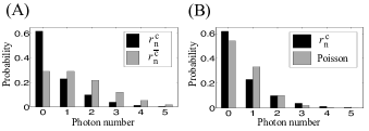
Figure 2: (A) Conditional photon number distribution in mode $a$ (see Fig. 1): $r^{c}_{n}$ (black) and $r^{\bar{c}}_{n}$ (grey) for the case $\mu_{1}=\mu_{2}=1$ and $t=1/2$. (B) $r^{c}_{n}$ (black) versus a Poissonian distribution of the same mean photon number (grey).

To perform decoy state QKD, we consider that Alice and Bob treat no click and click events separately, and they distill secret key from both of them. We use the secret key rate formula provided by Refs. [13, 14],

$$R\geq{}\textrm{max}\{R^{c},0\}+\textrm{max}\{R^{\bar{c}},0\},$$ (4)

with $R^{c}=q\{-Q^{c}f(E^{c})H(E^{c})+p^{c}_{1}Y_{1}[1-H(e_{1})]+p^{c}_{0}Y_{0}\}$, and similarly for $R^{\bar{c}}$. The parameter $q$ is the efficiency of the protocol ($q=1/2$ for the standard Bennett-Brassard 1984 protocol [15], and $q\approx{}1$ for its efficient version [16]), $Q^{c}$ is the overall gain of the signals, $E^{c}$ represents the overall quantum bit error rate (QBER), $f(E^{c})$ is the error correction efficiency [typically $f(E^{c})\geq{}1$ with Shannon limit $f(E^{c})=1$], $Y_{n}$ denotes the yield of a $n$-photon signal, i.e., the conditional probability of a detection event on Bob’s side given that Alice transmits an $n$-photon state, $e_{1}$ is the single photon error rate, and $H(x)=-x\log_{2}{(x)}-(1-x)\log_{2}{(1-x)}$ is the binary Shannon entropy function.

The quantities $Q^{c}$, $E^{c}$, $Q^{\bar{c}}$, and $E^{\bar{c}}$ are directly accessible from the experiment. They can be written as $Q^{c}=\sum_{n=0}^{\infty}p^{c}_{n}Y_{n}$ and $Q^{c}E^{c}=\sum_{n=0}^{\infty}p^{c}_{n}Y_{n}e_{n}$, and similarly for the case of a no click event. Here $e_{n}$ denotes the error rate of a $n$-photon signal ($e_{0}=1/2$ for random background). To apply the secret key rate formula given by Eq. (4) one needs to estimate a lower bound on $Y_{1}$, together with an upper bound on $e_{1}$. For that, we follow the procedure proposed in Ref. [17]. This method requires that $p^{t}_{n}$ and $p^{\bar{c}}_{n}$ satisfy certain conditions that we checked numerically. Note, however, that many other estimation techniques are also available, like, for instance, linear programming tools. We obtain

$$Y_{1}\geq{}Y^{l}_{1}\equiv\textrm{max}\Bigg{\{}0,\frac{p^{\bar{c}}_{2}Q^{t}-p^{t}_{2}Q^{\bar{c}}-(p^{\bar{c}}_{2}p^{t}_{0}-p^{t}_{2}p^{\bar{c}}_{0})Y_{0}^{u}}{p^{\bar{c}}_{2}p^{t}_{1}-p^{t}_{2}p^{\bar{c}}_{1}}\Bigg{\}},$$ (5)

where $Q^{t}=Q^{c}+Q^{\bar{c}}$, and $Y_{0}^{u}$ denotes an upper bound on the background rate $Y_{0}$ given by $Y_{0}^{u}=\textrm{min}\{(2E^{\bar{c}}Q^{\bar{c}})/p^{\bar{c}}_{0},(2E^{t}Q^{t})/p^{t}_{0}\}$. The error rate $e_{1}$ can be upper bounded as

$$e_{1}\leq{}e^{u}_{1}\equiv\textrm{min}\Bigg{\{}\frac{E^{\bar{c}}Q^{\bar{c}}-p^{\bar{c}}_{0}Y_{0}^{l}e_{0}}{p^{\bar{c}}_{1}Y_{1}^{l}},\frac{E^{c}Q^{c}-p^{c}_{0}Y_{0}^{l}e_{0}}{p^{c}_{1}Y_{1}^{l}},\frac{p^{\bar{c}}_{0}E^{t}Q^{t}-p^{t}_{0}E^{\bar{c}}Q^{\bar{c}}}{(p^{\bar{c}}_{0}p^{t}_{1}-p^{t}_{0}p^{\bar{c}}_{1})Y_{1}^{l}}\Bigg{\}},$$ (6)

with $Q^{t}E^{t}=Q^{c}E^{c}+Q^{\bar{c}}E^{\bar{c}}$, and where $Y_{0}^{l}$ denotes a lower bound on $Y_{0}$ given by $Y_{0}\geq{}Y^{l}_{0}\equiv\textrm{max}\{0,(p^{t}_{1}Q^{\bar{c}}-p^{\bar{c}}_{1}Q^{t})/(p^{t}_{1}p^{\bar{c}}_{0}-p^{\bar{c}}_{1}p^{t}_{0})\}$.

The only relevant statistics to evaluate $Y^{l}_{0}$, $Y^{l}_{1}$, and $e^{u}_{1}$ are $p^{t}_{n}$ and $p^{\bar{c}}_{n}$, with $n=0,1,2$. These probabilities can be obtained by solving Eqs. (2)-(3). After a short calculation, we find that $p^{\bar{c}}_{0}=e^{-\upsilon}$, $p^{\bar{c}}_{1}=\omega{}e^{-\upsilon}$, and $p^{\bar{c}}_{2}=(2\omega^{2}+\xi^{2})e^{-\upsilon}/4$, with $\omega=\mu_{1}{}t+\mu_{2}(1-t)$. The probabilities $p^{t}_{n}$ have the form $p^{t}_{0}=I_{0,\xi}e^{-\omega}$, $p^{t}_{1}=[\omega{}I_{0,\xi}-\xi{}I_{1,\xi}]e^{-\omega}$, and $p^{t}_{2}=[\omega^{2}I_{0,\xi}+(1-2\omega)\xi{}I_{1,\xi}+\xi^{2}{}I_{2,\xi}]e^{-\omega}/2$.

For simulation purposes we consider the channel model used in Refs. [3, 17]. This model reproduces a normal behaviour of the quantum channel, i.e., in the absence of eavesdropping. It allows us to calculate the observed experimental parameters $Q^{\bar{c}}$, $E^{\bar{c}}$, $Q^{t}$, and $E^{t}$. Our results, however, can also be applied to any other quantum channel, as they only depend on the observed gains and QBERs. In the scenario considered, the yields have the form $Y_{n}=1-(1-Y_{0})(1-\eta)^{n}$, where $\eta$ represents the overall transmittance of the system [3, 17]. This parameter can be related with a transmission distance $l$ measured in km for the given QKD scheme as $\eta=10^{-\frac{\alpha{}l}{10}}$, where $\alpha$ represents the loss coefficient of the optical fiber measured in dB/km. The product $Y_{n}e_{n}$ can be expressed as $Y_{n}e_{n}=Y_{0}e_{0}+(Y_{n}-Y_{0})e_{d}$, where $e_{d}$ is the probability that a photon hits the wrong detector due to the misalignment in the quantum channel and in Bob’s detection setup [3, 17]. After substituting these definitions into the gain and QBER formulas we obtain $Q^{\bar{c}}=F-(1-Y_{0})e^{(1-\eta)\omega-\upsilon}I_{0,(1-\eta)\xi}$, $Q^{\bar{c}}E^{\bar{c}}=(e_{0}-e_{d})Y_{0}F+e_{d}Q^{\bar{c}}$, $Q^{t}=1-(1-Y_{0})e^{-\eta\omega}I_{0,\eta\xi}$ and $Q^{t}E^{t}=(e_{0}-e_{d})Y_{0}+e_{d}Q^{t}$.

The resulting secret key rate is illustrated in Fig. 3.

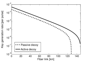
Figure 3: Lower bound on the secret key rate $R$ given by Eq. (4) in logarithmic scale for a passive decoy state setup with two intensity settings (dashed line). The transmittance of the BS is $t=1/2$. The solid line represents a lower bound on $R$ for an active asymptotic decoy state system [3].

The experimental parameters are [18]: $Y_{0}=1.7\times{}10^{-6}$, $e_{d}=0.033$, $\alpha=0.21$ dB/km, and Bob’s detection efficiency equal to $0.045$. We assume that $q=1$, $f(E^{c})=f(E^{\bar{c}})=1.22$, and $t=1/2$, i.e., we consider a simple $50:50$ BS. With this configuration, it turns out that the optimal values of the intensities $\mu_{1}$ and $\mu_{2}$ are almost constant with the distance. One of them is quite weak (around $10^{-4}$), while the other one is around $0.55$. Fig. 3 includes as well the case of an active asymptotic decoy state QKD system [3]. The cutoff points where the secret key rate drops down to zero are $l\approx{}128$ km (passive setup with two intensity settings) and $l\approx{}147$ km (active asymptotic setup). One could reduce this gap further by using a passive scheme with more intensity settings. For instance, one may employ a photon number resolving detector instead of a simple threshold photon detector, or use more threshold detectors in combination with BS. From these results we see that the performance of the passive scheme is comparable to the active one, thus showing the practical interest of the passive setup.

To conclude, we have analyzed a simple passive decoy state QKD system with phase randomized WCP. This setup represents an alternative to those active schemes based on the use of a variable optical attenuator. In the asymptotic limit of an infinite long experiment, we have shown that this passive system can provide a similar performance to the one achieved with an active source and infinity decoy settings. This idea can also be applied to other practical scenarios with different signals and detectors like, for example, those based on thermal states or even strong coherent pulses in conjunction with a regular photo-detector. Details of this analysis will be presented somewhere else.

The authors wish to thank R. Kaltenbaek, H.-K. Lo, B. Qi, and Y. Zhao for very useful discussions. M.C. especially thanks the Institute for Quantum Computing (University of Waterloo) for hospitality and support during his stay in this institution. This work was supported by the European Projects SECOQC and QAP, by the NSERC Discovery Grant, Quantum Works, CSEC, and by Xunta de Galicia (Spain, Grant No. INCITE08PXIB322257PR).

References

References

- [1] V. Scarani, H. Bechmann-Pasquinucci, N. J. Cerf, M. Dušek, N. Lütkenhaus and M. Peev, “The security of practical quantum key distribution”, Preprint quant-ph/0802.4155, accepted for publication in Rev. Mod. Phys.
- [2] W.-Y. Hwang, “Quantum key distribution with high loss: toward global secure communication”, Phys. Rev. Lett. 91, 057901 (2003).
- [3] H.-K. Lo, X. Ma and K. Chen, “Decoy state quantum key distribution”, Phys. Rev. Lett. 94, 230504 (2005).
- [4] X.-B. Wang, “Beating the photon-number-splitting attack in practical quantum cryptography”, Phys. Rev. Lett. 94, 230503 (2005).
- [5] Y. Zhao, B. Qi, X. Ma, H.-K. Lo and L. Qian, “Experimental quantum key distribution with decoy states”, Phys. Rev. Lett. 96, 070502 (2006).
- [6] D. Rosenberg, J. W. Harrington, P. R. Rice, P. A. Hiskett, C. G. Peterson, R. J. Hughes, A. E. Lita, S. W. Nam and J. E. Nordholt, “Long-distance decoy-state quantum key distribution in optical fiber”, Phys. Rev. Lett. 98, 010503 (2007).
- [7] T. Schmitt-Manderbach, H. Weier, M. Fürst, R. Ursin, F. Tiefenbacher, T. Scheidl, J. Perdigues, Z. Sodnik, C. Kurtsiefer, J. G. Rarity, A. Zeilinger and H. Weinfurter, “Experimental demonstration of free-space decoy-state quantum key distribution over 144 km”, Phys. Rev. Lett. 98, 010504 (2007).
- [8] W. Mauerer and C. Silberhorn, “Quantum key distribution with passive decoy state selection”, Phys. Rev. A 75, 050305(R) (2007).
- [9] Y. Adachi, T. Yamamoto, M. Koashi and N. Imoto, “Simple and efficient quantum key distribution with parametric down-conversion”, Phys. Rev. Lett. 99, 180503 (2007).
- [10] X. Ma and H.-K. Lo, “Quantum key distribution with triggering parametric down-conversion sources”, New J. Phys. 10, 073018 (2008).
- [11] Y. Adachi, T. Yamamoto, M. Koashi and N. Imoto, “Passive decoy-state quantum cryptography with pseudo-single-photon sources”, Proc. 8th Asian Conference on Quantum Information Science (AQIS’08), Seoul, 25 (2008).
- [12] G. Arfken, Mathematical Methods for Physicists, 3rd ed. (Academic Press, 1985).
- [13] D. Gottesman, H.-K. Lo, N. Lütkenhaus and J. Preskill, “Security of quantum key distribution with imperfect devices”, Quantum Inf. Comput. 4, 325 (2004).
- [14] H.-K. Lo, “Getting something out of nothing”, Quantum Inf. Comput. 5, 413 (2005).
- [15] C. H. Bennett and G. Brassard, “Quantum cryptography: public key distribution and coin tossing”, Proc. IEEE Int. Conference on Computers, Systems and Signal Processing, Bangalore, India, IEEE Press, New York, 175 (1984).
- [16] H.-K. Lo, H. F. C. Chau and M. Ardehali, “Efficient quantum key distribution scheme and a proof of Its unconditional security”, J. Cryptology 18, 133 (2005).
- [17] X. Ma, B. Qi, Y. Zhao and H.-K. Lo, “Practical decoy state for quantum key distribution”, Phys. Rev. A 72, 012326 (2005);
- [18] C. Gobby, Z. L. Yuan and A. J. Shields, “Quantum key distribution over 122 km of standard telecom fiber”, Appl. Phys. Lett. 84, 3762 (2004).