Asymptotics for the expected lifetime of Brownian motion on thin domains in $\mathbb{R}^{n}$

Abstract.

We derive a three-term asymptotic expansion for the expected lifetime of Brownian motion and for the torsional rigidity on thin domains in $\mathds{R}^{n}$, and a two-term expansion for the maximum (and corresponding maximizer) of the expected lifetime. The approach is similar to that which we used previously to study the eigenvalues of the Dirichlet Laplacian and consists of scaling the domain in one direction and deriving the corresponding asymptotic expansions as the scaling parameter goes to zero. Apart from being dominated by the one-dimensional Brownian motion along the direction of the scaling, we also see that the symmetry of the perturbation plays a role in the expansion.

As in the case of eigenvalues, these expansions may also be used to approximate the exit time for domains where the scaling parameter is not necessarilly close to zero.

• Denis Borisov (borisovdi@yandex.ru): Department of Physics and Mathematics, Bashkir State Pedagogical University, October rev. st., 3a, 450000, Ufa, Russia

• Pedro Freitas (freitas@cii.fc.ul.pt): Department of Mathematics, Faculdade de Motricidade Humana (TU Lisbon) and Group of Mathematical Physics of the University of Lisbon, Complexo Interdisciplinar, Av. Prof. Gama Pinto 2, P-1649-003 Lisboa, Portugal

1. Introduction

Let $\Omega$ be a bounded open set in $\mathbb{R}^{n}$ and consider the elliptic equation

(1.1) $$\begin{array}[]{rl}-\Delta u(x)=2,&x\in\Omega\vspace*{2mm}\\ u(x)=0,&x\in\partial\Omega\end{array}$$

Here and throughout the whole paper we use the notation $\Delta$ for the second order elliptic operator defined by

$$\Delta u=\displaystyle\sum_{i=1}^{n}\frac{\displaystyle\partial^{2}}{\displaystyle\partial x_{i}^{2}}u.$$

When the operator is acting only on some of these variables, this will be indicated by a subscript. Note that $\Delta=2\Delta^{P}$, where $\Delta^{P}$ denotes the probabilistic Laplacian, that is, the generator of the Brownian motion. Under certain mild conditions on the regularity of the boundary, the above equation has one and only one non-negative solution in $C(\overline{\Omega})$. However, except for a few domains such as ellipsoids, the solution is not known in closed form – see [AFR] for a recent result in the case of equilateral triangles.

On the other hand, solutions to equation (1.1) have a probabilistic interpretation in terms of the Brownian motion associated to the Laplacian in $\mathbb{R}^{n}$. More precisely, the value of $u$ at each point $x$ yields the expected lifetime of a particle starting from $x$. This, together with what was mentioned above regarding the (lack of) existence of explicit solutions, makes it of interest to be able to determine approximations for the exit time, where asymptotic approximations then play an important role – see, for instance, [GvH, GKP] and, for more recent work along these lines, [BEGK, U].

It is the purpose of the present paper to apply to this problem an approach that we have used recently in the case of Dirichlet eigenvalue problems and which provides quite accurate approximations for the first eigenvalue of the Laplace operator for certain classes of domains [BF1, BF2]. The idea consists in scaling the domain $\Omega$ along one direction and determining the asymptotic expansion of the solution in terms of the scaling parameter as it goes to zero. In this way we obtain an asymptotic expansion for the solution of equation (1.1) from which it is possible to derive expansions for other quantities such as the maximum of $u$, the corresponding maximizer and also the integral of $u$. In line with the above interpretation, the second of these quantities corresponds to the point in the domain with the largest expected lifetime, while the last one is known in the elasticity literature as the torsional rigidity – see [BBC] and the references therein.

Due to the way in which the perturbation is set up it is possible to reduce the problem of finding approximations of solutions of equation (1.1) to a sequence of one dimensional problems which may be solved explicitly. Because of this, we should then expect the expansions in question to be dominated by a term corresponding to a one-dimensional Brownian motion in the direction along which the scaling is being performed. This is indeed the case and we see that the first term in all these expansions does correspond to the solution of the respective one-dimensional problem – expected lifetime, maximum expected lifetime or torsion – on an interval whose length is the maximum of the height function along this direction.

The second term in the asymptotic expansions, on the other hand, has a more geometric interpretation as it also depends on a function that measures how asymmetric the domain is with respect to the hyperplane orthogonal to the scaling direction. In particular, we see that for a given height function, quantities such as the maximum expected lifetime or the torsion of thin domains are maximal if the domain is as symmetric as possible in this direction – see Theorems 1, 2 and 3 and the remarks following them.

As may be seen from the examples in Section 6, although our approximations are quite accurate for a fairly large range of values of the scaling parameter, the error can vary a lot as this parameter approaches one, depending on the domain under consideration – see the discussion in that section in term of the radius of convergence of the corresponding series.

To the best of our knowledge, the only similar situation that has been addressed previously in the literature was the case of thin tubular neighbourhoods (of constant section) of a compact submanifold of a Riemannian manifold. In this case, a two-term expansion was given in [GKP] for the asymptotic behaviour of the mean exit time as the width of the tube approached zero.

It should also be mentioned that there is a large number of papers devoted to the asymptotic expansions of the solutions to elliptic boundary value problems in thin domains – see [N], [NT] and the references therein. However, and to the best of our knowledge, the problem considered here has not been studied from this point of view.

The paper is organized as follows. In the next section we lay down the notation and state the main results of the paper. In Section 3 we prove the asymptotic expansion for solutions of the elliptic problem depending on a scaling parameter. Sections 4 and 5 then present the asymptotics for the maximum of this solution and for the torsional rigidity, respectively. We finish with an analysis of the error of these approximations for some specific domains.

2. Formulation of the problem and main results

Let $x=(x^{\prime},x_{n})$, $x^{\prime}=(x_{1},\ldots,x_{n-1})$ be Cartesian coordinates in $\mathds{R}^{n}$ and $\mathds{R}^{n-1}$, respectively, $\omega$ be a bounded domain in $\mathds{R}^{n-1}$ with $C^{1}$-boundary. By $h_{\pm}=h_{\pm}(x^{\prime})\in C(\overline{\omega})\cap C^{1}(\omega)$ we denote two arbitrary functions such that $H(x^{\prime}):=h_{-}(x^{\prime})+h_{+}(x^{\prime})>0$ for $x^{\prime}\in\omega$ and $H(x^{\prime})=0$ on $\partial\omega$. We also define the two functions

$$d(x^{\prime})=h_{+}(x^{\prime})-h_{-}(x^{\prime})\mbox{ and }p(x^{\prime})=h_{+}(x^{\prime})h_{-}(x^{\prime}).$$

Note that due to the relation $4p(x^{\prime})=H^{2}(x^{\prime})-d^{2}(x^{\prime})$ it is possible to interchange the functions in terms of which our results are presented. In general we chose those combinations which allowed to write the results in the most compact way. However, while the geometric interpretation of the $H$ and $d$ terms is quite clear, and in which in particular the function $d$ is a measure of the symmetry of the domain in the scaling direction, the meaning of the function $p$ is not as straightforward.

We now introduce a thin domain by

$$\Omega_{\varepsilon}:=\{x:x^{\prime}\in\omega,-\varepsilon h_{-}(x^{\prime})<x_{n}<\varepsilon h_{+}(x^{\prime})\},$$

where $\varepsilon$ is a small parameter, and consider the problem

(2.1) $$-\Delta u^{\varepsilon}=2\quad\text{in}\quad\Omega_{\varepsilon},\qquad u^{\varepsilon}=0\quad\text{on}\quad\partial\Omega_{\varepsilon}.$$

In view of the smoothness of the functions $h_{\pm}$ and the boundary of $\omega$ the domain $\Omega_{\varepsilon}$ satisfies the exterior sphere condition at every boundary point. Theorem 6.13 in [GT, Ch. 6, Sec. 6.3] implies that the solution to the problem (2.1) belongs to $C(\overline{\Omega_{\varepsilon}})$.

Assuming that the functions $h_{\pm}$ are smooth enough, we introduce a sequence of functions

(2.2) $$\alpha_{0}^{(2)}(x^{\prime}):=p(x^{\prime}),\quad\alpha_{1}^{(2)}(x^{\prime}):=d(x^{\prime}),\quad\alpha_{2}^{(2)}(x^{\prime}):=-1,$$

(2.3) $$\alpha_{i}^{(2j)}(x^{\prime}):=-\frac{\displaystyle 1}{\displaystyle i(i-1)}\Delta_{x^{\prime}}\alpha_{i-2}^{(2j-2)}(x^{\prime}),\quad i\geqslant 2,$$

(2.4) $$\alpha_{1}^{(2j)}(x^{\prime}):=-\sum\limits_{i=2}^{2j-1}\alpha_{i}^{(2j)}(x^{\prime})\sum\limits_{m=0}^{i-1}\big{(}h_{+}(x^{\prime})\big{)}^{m}\big{(}-h_{-}(x^{\prime})\big{)}^{i-m-1},$$

(2.5) $$\alpha_{0}^{(2j)}(x^{\prime}):=\sum\limits_{i=2}^{2j-1}\alpha_{i}^{(2j)}(x^{\prime})\sum\limits_{m=1}^{i-1}\big{(}h_{+}(x^{\prime})\big{)}^{m}\big{(}-h_{-}(x^{\prime})\big{)}^{i-m}.$$

The first of our results describes the uniform asymptotic expansion for $u^{\varepsilon}$ and forms the basis for the remaining expansions in the paper.

Theorem 1.

Given any $N\geqslant 1$, let the functions $h_{\pm}$ be such that$\alpha_{i}^{(2j)}\in C^{2}(\overline{\omega})$, $j\leqslant N$. Then the function $u^{\varepsilon}$ satisfies the asymptotic formula

(2.6) $$u^{\varepsilon}(x)=\sum\limits_{j=1}^{N}\varepsilon^{2j}u_{2j}\left(x^{\prime},\frac{x_{n}}{\varepsilon}\right)+\mathcal{O}(\varepsilon^{2N+2}),$$

(2.7) $$u_{2j}(x^{\prime},\xi_{n}):=\sum\limits_{i=0}^{2j-1}\alpha_{i}^{(2j)}(x^{\prime})\xi_{n}^{i},$$

in the $C(\overline{\Omega}_{\varepsilon})$-norm. In particular,

(2.8) $$\begin{array}[]{lll}u_{2}(x^{\prime},\xi_{n})&=&-\xi_{n}^{2}+\xi_{n}d(x^{\prime})+p(x^{\prime}),\vspace*{2mm}\\ u_{4}(x^{\prime},\xi_{n})&=&-\frac{\displaystyle\xi_{n}^{3}}{\displaystyle 6}\Delta_{x^{\prime}}d(x^{\prime})-\frac{\displaystyle\xi_{n}^{2}}{\displaystyle 2}\Delta_{x^{\prime}}p(x^{\prime})+\alpha_{1}^{(4)}(x^{\prime})\xi_{n}+\alpha_{0}^{(4)}(x^{\prime}),\vspace*{2mm}\\ u_{6}(x^{\prime},\xi_{n})&=&\frac{\displaystyle\xi_{n}^{5}}{\displaystyle 120}\Delta_{x^{\prime}}^{2}d(x^{\prime})+\frac{\displaystyle\xi_{n}^{4}}{\displaystyle 24}\Delta_{x^{\prime}}^{2}p(x^{\prime})\vspace*{2mm}\\ &&\hskip 5.69046pt-\frac{\displaystyle\xi_{n}^{3}}{\displaystyle 36}\Delta_{x^{\prime}}\left\{\left[d^{2}(x^{\prime})+p(x^{\prime})\right]\Delta_{x^{\prime}}d(x^{\prime})+3d(x^{\prime})\Delta_{x^{\prime}}p(x^{\prime})\right\}\vspace*{2mm}\\ &&\hskip 11.38092pt-\frac{\displaystyle\xi_{n}^{2}}{\displaystyle 12}\Delta_{x^{\prime}}\left[d(x^{\prime})p(x^{\prime})\Delta_{x^{\prime}}d(x^{\prime})+3p(x^{\prime})\Delta_{x^{\prime}}p(x^{\prime})\right]\vspace*{2mm}\\ &&\hskip 17.07182pt+\alpha^{(6)}_{1}(x^{\prime})\xi_{n}+\alpha^{(6)}_{0}(x^{\prime}),\end{array}$$

where

$$\begin{array}[]{lll}\alpha_{1}^{(4)}(x^{\prime})&=&\frac{\displaystyle 1}{\displaystyle 6}\left[d^{2}(x^{\prime})+p(x^{\prime})\right]\Delta_{x^{\prime}}d(x^{\prime})+\frac{\displaystyle 1}{\displaystyle 2}d(x^{\prime})\Delta_{x^{\prime}}p(x^{\prime}),\vspace*{2mm}\\ \alpha_{0}^{(4)}(x^{\prime})&=&\frac{\displaystyle 1}{\displaystyle 6}d(x^{\prime})p(x^{\prime})\Delta_{x^{\prime}}d(x^{\prime})+\frac{\displaystyle 1}{\displaystyle 2}p(x^{\prime})\Delta_{x^{\prime}}p(x^{\prime}),\vspace*{2mm}\\ \alpha_{1}^{(6)}(x^{\prime})&=&\frac{\displaystyle 1}{\displaystyle 12}d(x^{\prime})\Delta_{x^{\prime}}\left[d(x^{\prime})p(x^{\prime})\Delta_{x^{\prime}}d(x^{\prime})+3p(x^{\prime})\Delta_{x^{\prime}}p(x^{\prime})\right]\vspace*{2mm}\\ &&\hskip 5.69046pt+\frac{\displaystyle 1}{\displaystyle 36}\left[d^{2}(x^{\prime})+p(x^{\prime})\right]\Delta_{x^{\prime}}\left\{3d(x^{\prime})\Delta_{x^{\prime}}p(x^{\prime})+\left[d^{2}(x^{\prime})+p(x^{\prime})\right]\Delta_{x^{\prime}}d(x^{\prime})\right\}\vspace*{2mm}\\ &&\hskip 11.38092pt-\frac{\displaystyle 1}{\displaystyle 24}d(x^{\prime})\left[d^{2}(x^{\prime})+2p(x^{\prime})\right]\Delta^{2}_{x^{\prime}}p(x^{\prime})\vspace*{2mm}\\ &&\hskip 17.07182pt-\frac{\displaystyle 1}{\displaystyle 120}\left[d^{4}(x^{\prime})+3d^{2}(x^{\prime})p(x^{\prime})+p^{2}(x^{\prime})\right]\Delta_{x^{\prime}}^{2}d(x^{\prime}),\vspace*{2mm}\\ \alpha_{0}^{(6)}(x^{\prime})&=&\frac{\displaystyle p(x^{\prime})}{\displaystyle 12}\Delta_{x^{\prime}}\left[d(x^{\prime})p(x^{\prime})\Delta_{x^{\prime}}d(x^{\prime})+3p(x^{\prime})\Delta_{x^{\prime}}p(x^{\prime})\right]\vspace*{2mm}\\ &&\hskip 5.69046pt+\frac{\displaystyle d(x^{\prime})p(x^{\prime})}{\displaystyle 36}\Delta_{x^{\prime}}\left\{\left[d^{2}(x^{\prime})+p(x^{\prime})\right]\Delta_{x^{\prime}}d(x^{\prime})+3d(x^{\prime})\Delta_{x^{\prime}}p(x^{\prime})\right\}\vspace*{2mm}\\ &&\hskip 11.38092pt-\frac{\displaystyle 1}{\displaystyle 24}p(x^{\prime})\left[d^{2}(x^{\prime})+p(x^{\prime})\right]\Delta_{x^{\prime}}^{2}p(x^{\prime})\vspace*{2mm}\\ &&\hskip 17.07182pt-\frac{\displaystyle 1}{\displaystyle 120}d(x^{\prime})p(x^{\prime})\left[d^{2}(x^{\prime})+2p(x^{\prime})\right]\Delta_{x^{\prime}}^{2}d(x^{\prime}).\end{array}$$

The coefficients of the asymptotic expansion (2.6) involve two scales, namely, the variable $x^{\prime}$ and the rescaled variable $\xi_{n}:=x_{n}/\varepsilon$, so, this is a two-scale asymptotics. This is a very natural situation for the problem (2.1) since by passing to the variable $\xi_{n}$ we get a bounded domain

$$\Omega:=\{(x^{\prime},\xi_{n}):x^{\prime}\in\omega,-h_{-}(x^{\prime})<\xi_{n}<h_{+}(x^{\prime})\}.$$

In this domain there is no distinguished variable as was the case of $x_{n}$ in the domain $\Omega_{\varepsilon}$. This is one reason why the asymptotics for $u^{\varepsilon}$ involve two scales. Another way of understanding this fact is that while $x_{n}$ ranges in a small interval the remaining variable $x^{\prime}$ ranges in a bounded set. From this point of view, it is natural to rescale the variable $x_{n}$ and pass to $\xi_{n}$.

Let us discuss the probabilistic meaning of the first terms in the asymptotic expansion (2.6). As we will see in the proof of Theorem 1, the first term $u_{2}$ solves the boundary value problem (3.3) below. In view of Remark 8.7b) in [MP, Ch. 8, Sec. 8.1] the function $u_{2}(x^{\prime},\xi_{n})$ describes the Brownian motion on the interval $(-h_{-}(x^{\prime}),h_{+}(x^{\prime}))$ and it is the expected lifetime for the mentioned segment for a Brownian motion which started at the point $\xi_{n}$.

It is also possible to give a probabilistic-geometric interpretation of the next term $u_{4}$. This will be the solution to the boundary value problem (3.4) below, when $j=1$, namely,

$$- \frac{\partial^{2}u_{4}}{\partial\xi_{n}^{2}}=\xi_{n}\Delta_{x^{\prime}}d(x^{\prime})+\Delta_{x^{\prime}}p(x^{\prime}),\quad\xi\in\big{(}-h_{-}(x^{\prime}),h_{+}(x^{\prime})\big{)},$$

$$u_{4}=0,\quad\xi_{n}=\pm h_{\pm}(x^{\prime}),\quad x^{\prime}\in\omega.$$

Again by Remark 8.7a) in [MP, Ch. 8, Sec. 8.1] the function $u_{4}$ can be represented as

$$u_{4}(x^{\prime},\xi_{n})=\frac{1}{2}\Delta_{x^{\prime}}d(x^{\prime})\mathbb{E}_{\xi_{n}}\left[\int\limits_{0}^{T}B(t)\,\mathrm{d}t\right]+\frac{1}{2}\Delta_{x^{\prime}}p(x^{\prime})\mathbb{E}_{\xi_{n}}[T],$$

where $\{B(t):t\geqslant 0\}$ is the one-dimensional Brownian motion on the segment $(-h_{-}(x^{\prime}),h_{+}(x^{\prime}))$, $T:=\inf\{t:t>0,B(t)\not\in(-h_{-}(x^{\prime}),h_{+}(x^{\prime})\}$, $\mathbb{E}_{\xi_{n}}$ is the expectation associated with the probability measure $\mathbb{P}_{\xi_{n}}$ such that the process $\{B(t):t\geqslant 0\}$ is a Brownian motion started in $\xi_{n}$. The term

$$\frac{1}{2}\mathbb{E}_{\xi_{n}}[T]=u_{2}(x^{\prime})$$

is exactly the lifetime for this one-dimensional process, while

$$\mathbb{E}_{\xi_{n}}\left[\int\limits_{0}^{T}B(t)\,\mathrm{d}t\right]$$

is known in the literature as the occupation time for the Brownian motion which started at the point $\xi_{n}$ and left the interval at time $T$. The factors $\Delta_{x^{\prime}}p(x^{\prime})$ and $\Delta_{x^{\prime}}d(x^{\prime})$ then represent a geometric measure of the deviation from the symmetric domain, as mentioned in the Introduction. More precisely, if the domain is symmetric with respect to the hyperplane where $\omega$ lies, then the difference function $d$ vanishes, $p=H^{2}/4$ and $u_{4}$ reduces to the expected (one-dimensional) lifetime, affected by a factor which is proportional to the Laplacian of the square of the height function.

Continuing in the same way, that is, employing equations (3.4) for $u_{2j}$ and [MP, Ch. 8, Sec. 8.1, Rem. 8.7a)], it is possible to give similar interpretations for all other terms in the asymptotics (2.6).

From Theorem 1, we are then able to derive explicit asymptotic formulas for both the maximum of $u^{\varepsilon}$ and the torsional rigidity for the family of domains $\Omega_{\varepsilon}$ as $\varepsilon$ goes to zero.

Theorem 2.

Let the family of domains $\Omega_{\varepsilon}$ and the functions $h_{-},h_{+}$ and $H$ be as above. We assume further that $H$ satisfies the following hypotheses:

1. There exists a unique point $\overline{x}\in\omega$ at which $H$ achieves its global maximum which will be denoted by $H_{0}$;

2. The Hessian matrix of $H$ at $\overline{x}$, denoted by $2H_{2}$, is negative definite;

3. The functions $h_{\pm}$ are 5 times continuously differentiable in a vicinity of $\overline{x}$.

Then the maximum value of $u^{\varepsilon}$ in $\Omega_{\varepsilon}$ satisfies

$$\max_{x\in\Omega_{\varepsilon}}u^{\varepsilon}(x)=\frac{\displaystyle 1}{\displaystyle 4}H_{0}^{2}\varepsilon^{2}+\frac{\displaystyle 1}{\displaystyle 8}H_{0}^{2}\left[\frac{\displaystyle 1}{\displaystyle 2}\Delta(H_{0}^{2})-|\nabla d_{0}|^{2}\right]\varepsilon^{4}+\mathcal{O}(\varepsilon^{5}),$$

as $\varepsilon\to 0$. Here $\Delta(H_{0}^{2})$ denotes Laplacian of the height function squared at the point of maximum $\overline{x}$, while $\nabla d_{0}$ is the value of the gradient of $d$ at the same point.

Remark 2.1.

As mentioned in the Introduction, the first term in the expansion of the maximum corresponds to that of a one–dimensional Brownian motion on an interval of length $\varepsilon H_{0}$. The second term, on the other hand, has a geometrical interpretation and measures the (local) asymmetry of the domain in the direction in which the scaling is being carried out, in a neighbourhood of the point of maximum height. We note that this coefficient will be maximal when $\overline{x}$ is a critical point of the difference function $d$.

Remark 2.2.

If one drops the hypothesis that $H_{2}$ is nonsingular it will still be possible to obtain an expansion, but this will be much more involved and will depend on higher order terms in the expansion of $H$ around $\overline{x}$.

Remark 2.3.

The hypothesis on a unique maximum of $H$ may also be dropped and provided there is only a finite number of such maxima the results still hold except that one has to construct different expansions for each maximum. The case of a continuum of maxima is also possible to handle with the techniques employed here but requires some further changes to the approach.

Remark 2.4.

In the process of proving the above theorem we also obtain a two-term asymptotic expansion for the maximizer – see Theorem 4. However, this depends on higher order terms in the expansions of both $d$ and $p$ and requires the introduction of more detailed notation which we postpone till Section 4 below.

Remark 2.5.

Under the hypotheses H1 and H2 of Theorem 2 and assuming that the functions $h_{\pm}$ are smooth enough in a vicinity of $\overline{x}$, it is possible to construct more terms in the asymptotic expansions for the maximum of $u^{\varepsilon}$ in $\Omega_{\varepsilon}$ and for the corresponding maximizer. In order to do this, one should follow the main lines of the proof of Theorem 2, employing Lemma 4.2 as a starting point. At the same time, it requires bulky and technical calculations which we would like to avoid. This is the reason why we provide only two-term asymptotics in Theorem 2.

Finally, the integration of the asymptotic expansion for $u^{\varepsilon}$ given by Theorem 1 yields the corresponding asymptotic expansion for the torsional rigidity.

Theorem 3 (Torsional rigidity).

Under the conditions of Theorem 1 we have

$$\displaystyle\int_{\Omega_{\varepsilon}}u^{\varepsilon}(x)\;{\rm d}x= \frac{\displaystyle\varepsilon^{3}}{\displaystyle 6}\displaystyle\int_{\omega}H^{3}(y)\;{\rm d}y$$

$$\hskip 7.11317pt+\frac{\displaystyle\varepsilon^{5}}{\displaystyle 24}\displaystyle\int_{\omega}H^{3}(y)\left[\frac{\displaystyle 1}{\displaystyle 2}\Delta_{y}[H^{2}(y)]-|\nabla_{y}d(y)|^{2}\right]\;{\rm d}y$$

$$\hskip 14.22636pt+\varepsilon^{7}\displaystyle\int_{\omega}H(y)\left\{\frac{\displaystyle 1}{\displaystyle 720}\left[H^{2}(y)d^{3}(y)+3d(y)p^{2}(y)\right]\Delta_{y}^{2}d(y)\right.$$

$$\hskip 21.33955pt+\frac{\displaystyle 1}{\displaystyle 120}\left\{H^{2}(y)d^{2}(y)+p(y)\left[p(y)-d^{2}(y)\right]\right\}\Delta_{y}^{2}p(y)$$

$$\hskip 21.33955pt-\frac{\displaystyle 1}{\displaystyle 144}\left[H^{2}(y)d(y)-2d(y)p(y)\right]$$

$$\hskip 28.45274pt\times\Delta_{y}\left\{\left[d^{2}(y)+p(y)\right]\Delta_{y}d(y)+3d(y)\Delta_{y}p(y)\right\}$$

$$\hskip 21.33955pt-\frac{\displaystyle 1}{\displaystyle 36}\left[H^{2}(y)-3p(y)\right]$$

$$\hskip 28.45274pt\times\Delta_{y}\left[d(y)p(y)\Delta_{y}d(y)+3p(y)\Delta_{y}p(y)\right]$$

$$\left.\hskip 21.33955pt+\frac{\displaystyle 1}{\displaystyle 2}d(y)\alpha_{1}^{(6)}(y)+\alpha^{(6)}_{0}(y)\right\}\;{\rm d}y$$

$$\hskip 28.45274pt+\mathcal{O}(\varepsilon^{8}),$$

where $\alpha^{(6)}_{0}$ and $\alpha_{1}^{(6)}$ are as in Theorem 1.

Remark 2.6.

Again we see that the first term in the expansion corresponds to the one–dimensional Brownian motion on the line segment with maximal height in the direction of scaling. Also as before, the second term measures the degree of symmetry of the domain with respect to the hyperplane orthogonal to this direction, and we see that, for a given height function, this term is maximal when the difference function vanishes that is, when the domain is symmetric with respect to this hyperplane.

Remark 2.7.

In order to obtain the average expected lifetime it remains to divide by the volume of $\Omega_{\varepsilon}$ which is given by

$$|\Omega_{\varepsilon}|=\displaystyle\int_{\Omega_{\varepsilon}}\;{\rm d}x=\displaystyle\int_{\omega}\displaystyle\int_{-\varepsilon h_{-}(x^{\prime})}^{\varepsilon h_{+}(x^{\prime})}\;{\rm d}\xi_{n}\;{\rm d}x^{\prime}=\varepsilon\displaystyle\int_{\omega}H(y)\;{\rm d}y.$$

3. The asymptotic expansion for $u^{\varepsilon}$

In this section we prove Theorem 1. We begin by passing to the variables $(x^{\prime},\xi_{n})$ in (2.1) leading us to

(3.1) $$\left(-\varepsilon^{2}\Delta_{x^{\prime}}-\frac{\partial^{2}}{\partial\xi_{n}^{2}}\right)u^{\varepsilon}=2\varepsilon^{2}\quad\text{in}\quad\Omega,\qquad u^{\varepsilon}=0\quad\text{on}\quad\partial\Omega.$$

We construct the asymptotic expansion to the problem (3.1) as follows

(3.2) $$u^{\varepsilon}(x)=\sum\limits_{j=0}^{\infty}\varepsilon^{2j}u_{2j}(x^{\prime},\xi_{n}),$$

where $u^{j}(x^{\prime},\xi_{n})$ are functions to be determined.

We substitute the expansion (3.2) into (3.1) and equate the coefficients of like powers in $\varepsilon$. This yields the following boundary value problems for $u_{2j}$:

(3.3) $$\begin{aligned} -&\frac{\partial^{2}u_{2}}{\partial\xi_{n}^{2}}=2,\quad\xi\in\big{(}-h_{-}(x^{\prime}),h_{+}(x^{\prime})\big{)},\\ &u_{2}=0,\quad\xi_{n}=\pm h_{\pm}(x^{\prime}),\quad x^{\prime}\in\omega,\end{aligned}$$

(3.4) $$\begin{aligned} -&\frac{\partial^{2}u_{2j}}{\partial\xi_{n}^{2}}=\Delta_{x^{\prime}}u_{2j-2},\quad\xi\in\big{(}-h_{-}(x^{\prime}),h_{+}(x^{\prime})\big{)},\\ &u_{2j}=0,\quad\xi_{n}=\pm h_{\pm}(x^{\prime}),\quad x^{\prime}\in\omega,\quad j\geqslant 2.\end{aligned}$$

It is easy to check that the solution to (3.3) is

$$u_{2}(x^{\prime},\xi_{n}^{\prime})=-\xi_{n}^{2}+d(x^{\prime})\xi_{n}+p(x^{\prime})$$

that proves (2.7) for $j=1$. Substituting this formula into the (3.4) for $j=2$, we get

(3.5) $$- \frac{\partial^{2}u_{4}}{\partial\xi_{n}^{2}}=\xi_{n}\Delta_{x^{\prime}}d(x^{\prime})+\Delta_{x^{\prime}}p(x^{\prime}),\quad\xi\in\big{(}-h_{-}(x^{\prime}),h_{+}(x^{\prime})\big{)},$$

$$u_{4}=0,\quad\xi_{n}=\pm h_{\pm}(x^{\prime}),\quad x^{\prime}\in\omega.$$

The solution to the obtained equation is

$$u_{4}(x^{\prime},\xi_{n})=\frac{\xi_{n}^{3}}{6}\Delta_{x^{\prime}}d(x^{\prime})+\frac{\xi_{n}^{2}}{2}\Delta_{x^{\prime}}p(x^{\prime})+C_{1}^{(4)}(x^{\prime})\xi_{n}+C_{0}^{(4)}(x^{\prime}),$$

where $C_{i}^{(4)}$ are arbitrary functions. We determine them by the boundary conditions in (3.5) and it implies (2.7) for $j=2$.

We prove the remaining formulas (2.7) by induction. Assuming that they are valid for $j\leqslant k$, we consider the equation in (3.4) for $j=k+1$ and see that its general solution reads as follows,

(3.6) $$u_{2k+2}(x^{\prime},\xi_{n})= -\sum\limits_{i=0}^{2k-1}\frac{\xi_{n}^{i+2}}{i(i+2)}\Delta_{x^{\prime}}\alpha_{i}^{(2k-2)}+C_{1}^{(2k+2)}\xi_{n}+C_{0}^{(2k+2)}(x^{\prime})$$

$$= \sum\limits_{i=2}^{2k+1}\alpha_{i}^{(2k+1)}\xi_{n}^{i}+C_{1}^{(2k+2)}\xi_{n}+C_{0}^{(2k+2)}(x^{\prime}),$$

where $C_{i}^{(2k+2)}$ are arbitrary functions. The boundary conditions in (3.4) imply the equations for $C_{i}^{(2k+2)}$,

$$C_{1}^{(2k+2)}h_{+}+C_{0}^{(2k+2)}=-\sum\limits_{i=2}^{2k+2}\alpha_{i}^{(2k+2)}h_{+}^{i},$$

$$- C_{1}^{(2k+2)}h_{-}+C_{0}^{(2k+2)}=-\sum\limits_{i=2}^{2k+2}\alpha_{i}^{(2k+2)}(-h_{-})^{i}.$$

We solve it and get,

$$C_{1}^{(2k+2)}= -\sum\limits_{i=2}^{2k+2}\alpha_{i}^{(2k+2)}\frac{h_{+}^{i}-(-h_{-})^{i}}{h_{+}+h_{-}}$$

$$= -\sum\limits_{i=2}^{2k+1}\alpha_{i}^{(2j)}(x^{\prime})\sum\limits_{m=0}^{i-1}\big{(}h_{+}(x^{\prime})\big{)}^{m}\big{(}-h_{-}(x^{\prime})\big{)}^{i-m-1}=\alpha_{1}^{(2k+2)},$$

$$C_{0}^{(2k+2)}= -\sum\limits_{i=2}^{2k+2}\alpha_{i}^{(2k+2)}\left(h_{+}^{i}-\sum\limits_{m=0}^{i-1}h_{+}^{m+1}(-h_{-})^{i-m-1}\right)$$

$$= \sum\limits_{i=2}^{2k+1}\alpha_{i}^{(2j)}(x^{\prime})\sum\limits_{m=1}^{i-1}\big{(}h_{+}(x^{\prime})\big{)}^{m}\big{(}-h_{-}(x^{\prime})\big{)}^{i-m}=\alpha_{0}^{(2k+2)}.$$

We substitute the obtained identities into (3.6) and arrive at (2.7) for $j=k+1$.

Given any $N\geqslant 1$, assume that $\alpha_{i}^{(2j)}\in C^{2}(\overline{\omega})$, $j\geqslant N$. Let

(3.7) $$u^{\varepsilon,N}(x^{\prime},\xi_{n}):=\sum\limits_{j=0}^{N}\varepsilon^{2j}u_{2j}(x^{\prime},\xi_{n}).$$

It follows from the problems (3.3), (3.4) that the function $u^{\varepsilon,N}$ solves the boundary value problem

$$\left(-\varepsilon^{2}\Delta_{x^{\prime}}-\frac{\partial^{2}}{\partial\xi_{n}^{2}}\right)u^{\varepsilon,N}=2\varepsilon^{2}+\varepsilon^{2N+2}\Delta_{x^{\prime}}u_{2N}\quad\text{in}\quad\Omega,\qquad u^{\varepsilon,N}=0\quad\text{on}\quad\partial\Omega.$$

Hence, the function $\widetilde{u}^{\varepsilon,N}:=u^{\varepsilon}-u^{\varepsilon,N}$ is the solution to

(3.8) $$\left(\varepsilon^{2}\Delta_{x^{\prime}}+\frac{\partial^{2}}{\partial\xi_{n}^{2}}\right)\widetilde{u}^{\varepsilon,N}=\varepsilon^{2N+2}\Delta_{x^{\prime}}u_{2N}\quad\text{in}\quad\Omega,\qquad\widetilde{u}^{\varepsilon,N}=0\quad\text{on}\quad\partial\Omega.$$

The coefficient affecting the derivative $\frac{\partial^{2}}{\partial\xi_{n}^{2}}$ in the last equation is one. Employing this fact and applying the maximum principle in the form of inequality (1.9) in [LU, Ch. 3, Sec. 1], we obtain the estimate

(3.9) $$\|\widetilde{u}^{\varepsilon,N}\|_{C(\overline{\Omega})}\leqslant C\varepsilon^{2N+2}\|\Delta_{x^{\prime}}u_{2N}\|_{C(\overline{\Omega})}\leqslant C\varepsilon^{2N+2},$$

where the constant $C$ is independent of $\varepsilon$. It proves the formula (2.6). The formulas (2.8) follow directly from (2.2), (2.3), (2.4), (2.5), (2.7). The proof is complete.

4. Proof of Theorem 2

In the whole of this section we shall consider the function $u^{\varepsilon}(x^{\prime},\xi_{n})$. This is then defined on $\Omega$ and it is clear that it is sufficient to find the maximum of $u^{\varepsilon}(x^{\prime},\xi_{n})$ since after rescalling $x_{n}\to x_{n}\varepsilon$ the maximum of the function remains unaltered.

4.1. Existence of an expansion and terms of order $\varepsilon^{2}$

We begin by showing that, under the hypothesis of Theorem 2 and up to order $\varepsilon^{2}$, the maximum of $u$ has an asymptotic expansion that may be obtained directly from the expression of $u_{2}$.

Lemma 4.1.

Under the hypothesis of Theorem 2 we have

$$\max_{x\in\Omega_{\varepsilon}}u^{\varepsilon}(x)=\max_{x\in\Omega}u_{2}(x)\varepsilon^{2}+\mathcal{O}(\varepsilon^{4})\mbox{ as }\varepsilon\to 0.$$

Furthermore

$$\max_{x\in\Omega}u_{2}(x)=u_{2}\left(\overline{x},\frac{d(\overline{x})}{2}\right)=\frac{\displaystyle 1}{\displaystyle 4}H_{0}^{2}$$

and is unique.

Proof.

The first part follows directly from the asymptotics of $u^{\varepsilon}$ given by Theorem 1, since we now have

$$u^{\varepsilon}(x^{\prime},\xi_{n})=\varepsilon^{2}u_{2}(x^{\prime},\xi_{n})+\mathcal{O}(\varepsilon^{4}).$$

For the second part, note that we may write

$$\begin{array}[]{lll}u_{2}(x^{\prime},\xi_{n})&=&-\left[\xi_{n}^{2}+\xi_{n}\left(h_{-}(x^{\prime})-h_{+}(x^{\prime})\right)+h_{-}(x^{\prime})h_{+}(x^{\prime})\right]\vspace*{2mm}\\ &=&-\left[\xi_{n}-\frac{\displaystyle 1}{\displaystyle 2}d(x)\right]^{2}+\frac{\displaystyle 1}{\displaystyle 4}H^{2}(x).\end{array}$$

This last expression is clearly maximized when $\xi_{n}=d(x)/2$ and $H$ is also maximized, yielding $x^{\prime}=\overline{x}$ and $\xi=d(\overline{x})/2$. The uniqueness follows directly from hypothesis H1. ∎

In order to go on to obtain the next terms in the expansion for the maximum (and the corresponding maximizer), we need to show the existence of such an expansion which we do in the next lemma. This also proves that the coefficients of the terms of order one in both the expansions for $x^{\prime}$ and $\xi_{n}$ vanish.

Lemma 4.2.

Given any $N\geqslant 1$, assume that the functions $h_{\pm}$ are $[N/2]+2N$ times continuously differentiable in a vicinity of the point $\overline{x}$, and the hypotheses H1 and H2 of Theorem 2 hold true. Then the function $u^{\varepsilon,N}$ has only one stationary point which is a maximum. The corresponding maximizer has the following asymptotic expansion

(4.1) $$\overline{x}^{\varepsilon,N}=\overline{x}+\sum\limits_{i=1}^{[N/2]}\varepsilon^{2i}\overline{x}_{2i}+\mathcal{O}(\varepsilon^{2[N/2]+2}),$$

$$\overline{\xi}^{\varepsilon,N}=\frac{d(\overline{x})}{2}+\sum\limits_{i=1}^{[N/2]}\varepsilon^{2i}\xi_{ni}+\mathcal{O}(\varepsilon^{2[N/2]+2}).$$

The maximum of the function $u^{\varepsilon}$ satisfies the identity

(4.2) $$\max\limits_{\Omega_{\varepsilon}}u^{\varepsilon}(x)=\max\limits_{\Omega}u^{\varepsilon}(x^{\prime},\varepsilon\xi_{n})=\max\limits_{\Omega}u^{\varepsilon,N}(x^{\prime},\xi_{n})+\mathcal{O}(\varepsilon^{2N+2}),$$

and any maximizer $(\overline{x}^{\varepsilon},\overline{\xi}^{\varepsilon})$ of this function has the asymptotic expansion

(4.3) $$\overline{x}^{\varepsilon}=\overline{x}+\sum\limits_{i=1}^{[N/2]}\varepsilon^{2i}\overline{x}_{2i}+\mathcal{O}(\varepsilon^{N+1}),$$

$$\overline{\xi}^{\varepsilon}=\frac{d(\overline{x})}{2}+\sum\limits_{i=1}^{[N/2]}\varepsilon^{2i}\xi_{ni}+\mathcal{O}(\varepsilon^{N+1}).$$

Proof.

The identity (4.2) follows directly from the asymptotics (2.6) for $u^{\varepsilon}$.

Let us find the maximum of $u^{\varepsilon,N}$. In order to do this, we should first find the stationary points of this functions by solving the equation

$$\nabla_{(x^{\prime},\xi_{n})}u^{\varepsilon,N}(x^{\prime},\xi_{n})=0,$$

which is equivalent to

(4.4) $$\sum\limits_{i=1}^{N}\varepsilon^{2i-2}\nabla_{(x^{\prime},\xi_{n})}u_{2i}(x^{\prime},\xi_{n})=0.$$

It follows from Lemma 4.1 that for $\varepsilon=0$ this equation has a unique solution $(\overline{x},d(\overline{x})/2)$. In order to solve (4.4) for $\varepsilon>0$ we apply the implicit function theorem considering $(x^{\prime},\xi_{n})$ as functions of $\varepsilon$. We first need to check that the corresponding Jacobian is non-zero. It is easy to see that this Jacobian at $\varepsilon$ equal to zero coincides with the determinant of $2H_{2}$ which is non-zero by hypothesis H2.

The assumption for the smoothness of $h_{\pm}$ and the formulas (2.7), (2.2), (2.3), (2.4), (2.5) for $u_{2i}$ yield that $u_{2i}(x^{\prime},\xi_{n})$, $i=1,\ldots,N$, are $[N/2]+2$ times continuously differentiable in a small vicinity of $(\overline{x},d(\overline{x})/2)$. The dependence of the left hand side of (4.4) on $\varepsilon^{2}$ is holomorphic and by the implicit function theorem we conclude that for $\varepsilon$ small enough there exists a unique solution $(\overline{x}^{\varepsilon,N},\overline{\xi}^{\varepsilon,N})$ to (4.4) which is $[N/2]+1$ times continuously differentiable in $\varepsilon^{2}$. Hence, we have the Taylor polynomial (4.1). The point $(\overline{x}^{\varepsilon,N},\overline{\xi}^{\varepsilon,N})$ is the maximizer for $u^{\varepsilon,N}$ since by hypothesis H2 the Hessian of $u^{\varepsilon,N}$ at this point differs from $2H_{2}$ by an error of order $\mathcal{O}(\varepsilon^{2})$. We employ this fact and expand $u^{\varepsilon,N}(x^{\prime},\xi_{n})$ in Taylor series at $(\overline{x}^{\varepsilon,N},\overline{\xi}^{\varepsilon,N})$. As a result, we have the estimate

(4.5) $$u^{\varepsilon,N}(x^{\prime},\xi_{n})-u^{\varepsilon,N}(\overline{x}^{\varepsilon,N},\overline{\xi}^{\varepsilon,N})\leqslant-C_{1}\left(|x^{\prime}-\overline{x}^{\varepsilon,N}|^{2}+|\xi_{n}-\overline{\xi}^{\varepsilon,N}|^{2}\right),$$

where $C_{1}$ is a positive constant independent of $\varepsilon$, $x^{\prime}$ and $\xi_{n}$. This estimate is valid in a small fixed neighborhood $Q$ of the point $(\overline{x},d(\overline{x})/2)$. Since the function $u^{\varepsilon,N}$ has the maximum at $(\overline{x}^{\varepsilon,N},\overline{\xi}^{\varepsilon,N})$, we can choose the neighborhood $Q$ so that outside it the estimate

(4.6) $$u^{\varepsilon,N}(x^{\prime},\xi_{n})-u^{\varepsilon,N}(\overline{x}^{\varepsilon,N},\overline{\xi}^{\varepsilon,N})\leqslant-C_{2}<0$$

holds true, where the constant $C_{2}$ is independent of $\varepsilon$. Let us choose $(x^{\prime},\xi_{n})$ so that

(4.7) $$|x^{\prime}-\overline{x}^{\varepsilon,N}|^{2}+|\xi_{n}-\overline{\xi}^{\varepsilon,N}|^{2}\geqslant C_{3}\varepsilon^{2N+2},$$

where $C_{3}$ is a positive constant independent of $\varepsilon$, $x^{\prime}$ and $\xi_{n}$. Then it follows from (4.5), (4.6) that for such $(x^{\prime},\xi_{n})$ the inequality

$$u^{\varepsilon,N}(x^{\prime},\xi_{n})\leqslant u^{\varepsilon,N}(\overline{x}^{\varepsilon,N},\overline{\xi}^{\varepsilon,N})-C_{1}C_{3}\varepsilon^{2N+2}$$

is valid. Together with (4.2) it implies that a maximizer $(x_{\varepsilon}^{\prime},\xi_{\varepsilon})$ of $u^{\varepsilon}$ can not satisfy (4.7) for sufficiently small $\varepsilon$ and sufficiently large $C_{3}$ and therefore

(4.8) $$|x^{\prime}_{\varepsilon}-\overline{x}^{\varepsilon,N}|^{2}+|\xi_{\varepsilon}-\overline{\xi}^{\varepsilon,N}|^{2}\leqslant C_{3}\varepsilon^{2N+2}.$$

This inequality and (4.1) prove (4.3). ∎

4.2. The terms of order $\varepsilon^{4}$

In order to determine $\overline{x}_{2}$ and $\xi_{2}$ we shall need the terms of order $\varepsilon^{4}$ in the asymptotics of the gradient of $u^{\varepsilon}$, for which we need to consider $u_{4}$. We must also develop $d$ and $p$ around $\overline{x}$. In full generality, and to obtain the full asymptotic expansion, these developments should be written in terms of homogeneous polynomials of increasing degree. However, to obtain the first two terms in the asymptotics we will only need terms up to the homogeneous polynomials of third degree. Therefore, we shall choose a form that will be more convenient for our calculations. Write thus $d$ and $p$ as follows.

(4.9) $$\begin{array}[]{lll}d(x^{\prime})=d_{0}+d_{1}^{t}(x^{\prime}-\overline{x})+(x^{\prime}-\overline{x})^{t}D_{2}(x^{\prime}-\overline{x})+D_{3}(x^{\prime}-\overline{x})+\mathcal{O}(|x^{\prime}-\overline{x}|^{4}),\vspace*{2mm}\\ p(x^{\prime})=p_{0}+p_{1}^{t}(x^{\prime}-\overline{x})+(x^{\prime}-\overline{x})^{t}P_{2}(x^{\prime}-\overline{x})+P_{3}(x^{\prime}-\overline{x})+\mathcal{O}(|x^{\prime}-\overline{x}|^{4}),\end{array}$$

where $d_{1}=\nabla_{x^{\prime}}d(\overline{x})$, $p_{1}=\nabla_{x^{\prime}}p(\overline{x})$, $2D_{2}$ and $2P_{2}$ are the Hessian matrices of $d$ and $p$ at the point $\overline{x}$, respectively, and $D_{3}$ and $P_{3}$ are homogeneous polynomials of degree three to be specified below.

Due to the relation between $d$ and $p$ via the functions $h_{\pm}$ and the fact that $H^{\prime}(\overline{x})=h^{\prime}_{-}(\overline{x})+h^{\prime}_{+}(\overline{x})$ must vanish, we easily obtain that

$$p_{1}=-\frac{\displaystyle 1}{\displaystyle 2}d_{0}d_{1}.$$

In the case of $u_{4}$, the relevant derivatives are given by

$$\begin{array}[]{lll}\frac{\displaystyle\partial u_{4}}{\displaystyle\partial\xi_{n}}(x^{\prime},\xi_{n})&=&-\frac{\displaystyle 1}{\displaystyle 2}\xi_{n}^{2}\Delta_{x^{\prime}}d(x^{\prime})-\xi_{n}\Delta_{x^{\prime}}p(x^{\prime})+\alpha_{1}^{(4)}(x^{\prime})\vspace*{2mm}\\ \nabla_{x}u_{4}(x^{\prime},\xi_{n})&=&-\frac{\displaystyle 1}{\displaystyle 6}\xi_{n}^{3}\nabla_{x^{\prime}}\left[\Delta_{x^{\prime}}d(x^{\prime})\right]-\frac{\displaystyle 1}{\displaystyle 2}\xi_{n}^{2}\nabla_{x^{\prime}}\left[\Delta_{x^{\prime}}p(x^{\prime})\right]\vspace*{2mm}\\ &&\hskip 28.45274pt+\xi_{n}\nabla_{x^{\prime}}\alpha_{1}^{(4)}(x^{\prime})+\nabla_{x^{\prime}}\alpha_{0}^{(4)}(x^{\prime}).\end{array}$$

We shall first obtain the term of order $\varepsilon^{4}$ in the derivative of $u^{\varepsilon}$ with respect to $\xi_{n}$. This will have a component coming from the term of order $\varepsilon^{2}$ in the corresponding derivative of $u_{2}$, and another from the constant term in the derivative of $u_{4}$. In the first case it is straightforward to obtain that the required coefficient is given by

(4.10) $$-2\xi_{n2}+d_{1}^{t}\overline{x}_{2}.$$

In the case of $u_{4}$ the term coming from $\alpha_{1}^{(4)}$ is given by

$$\alpha_{1}^{(4)}(\overline{x}+\mathcal{O}(\varepsilon^{2}))=\frac{\displaystyle 1}{\displaystyle 3}\left(d_{0}^{2}+p_{0}\right)\operatorname{tr}(D_{2})+d_{0}\operatorname{tr}(P_{2})+\mathcal{O}(\varepsilon^{2}).$$

We thus obtain

$$\begin{array}[]{lll}\frac{\displaystyle\partial u_{4}}{\displaystyle\partial\xi_{n}}(\overline{x}+\mathcal{O}(\varepsilon^{2}),\frac{\displaystyle 1}{\displaystyle 2}d_{0}+\mathcal{O}(\varepsilon^{2}))&=&-\frac{\displaystyle 1}{\displaystyle 4}d_{0}^{2}\operatorname{tr}(D_{2})-d_{0}\operatorname{tr}(P_{2})\vspace*{2mm}\\ &&\hskip 14.22636pt+\frac{\displaystyle 1}{\displaystyle 3}\left(d_{0}^{2}+p_{0}\right)\operatorname{tr}(D_{2})\vspace*{2mm}\\ &&\hskip 28.45274pt+d_{0}\operatorname{tr}(P_{2})+\mathcal{O}(\varepsilon^{2})\vspace*{2mm}\\ &=&\frac{\displaystyle 1}{\displaystyle 12}\left(d_{0}^{2}+4p_{0}\right)\operatorname{tr}(D_{2})+\mathcal{O}(\varepsilon^{2})\end{array}$$

This, together with (4.10), yields

(4.11) $$\begin{array}[]{l}\frac{\displaystyle\partial u^{\varepsilon}}{\displaystyle\partial\xi_{n}}(\overline{x}+\overline{x}_{2}\varepsilon^{2}+\mathcal{O}(\varepsilon^{3}),\frac{\displaystyle 1}{\displaystyle 2}d_{0}+\xi_{n2}\varepsilon^{2}+\mathcal{O}(\varepsilon^{3}))=\vspace*{2mm}\\ \hskip 42.67912pt=\left[-2\xi_{n2}+d_{1}^{t}\overline{x}_{2}+\frac{\displaystyle 1}{\displaystyle 12}\left(d_{0}^{2}+4p_{0}\right)\operatorname{tr}(D_{2})\right]\varepsilon^{4}+\mathcal{O}(\varepsilon^{5}).\end{array}$$

We will now proceed to compute the gradient with respect to $x^{\prime}$. The case of $u_{2}$ is again straightforward and we obtain

(4.12) $$\begin{array}[]{l}\nabla_{x^{\prime}}u_{2}(\overline{x}+\overline{x}_{2}\varepsilon^{2}+\mathcal{O}(\varepsilon^{3}),\frac{\displaystyle 1}{\displaystyle 2}d_{0}+\xi_{n2}\varepsilon^{2}+\mathcal{O}(\varepsilon^{3}))=\vspace*{2mm}\\ \hskip 19.91684pt=\left(\frac{\displaystyle 1}{\displaystyle 2}d_{0}+\xi_{n2}\varepsilon^{2}\right)\left[d_{1}+2D_{2}\overline{x}_{2}\varepsilon^{2}\right]-\frac{\displaystyle 1}{\displaystyle 2}d_{0}d_{1}+2P_{2}\overline{x}_{2}\varepsilon^{2}+\mathcal{O}(\varepsilon^{3})\vspace*{2mm}\\ \hskip 19.91684pt=\left(\xi_{n2}d_{1}+d_{0}D_{2}\overline{x}_{2}+2P_{2}\overline{x}_{2}\right)\varepsilon^{2}+\mathcal{O}(\varepsilon^{3}).\end{array}$$

In the case of $u_{4}$ we are only interested in the terms of order $\varepsilon^{0}$. However, there are now expressions of the form

$$\nabla_{x^{\prime}}\Delta_{x^{\prime}}d(x^{\prime})\mbox{ and }\nabla_{x^{\prime}}\Delta_{x^{\prime}}p(x^{\prime}),$$

this being the reason why we need the homogeneous polynomials of third degree in the expansions of $d$ and $p$. On the other hand, this implies that the only relevant terms from $D_{3}$ and $P_{3}$ are those where one of the variables appears at least twice. If we write

$$\begin{array}[]{lll}D_{3}(x^{\prime})&=&\displaystyle\sum_{ijk}^{n-1}d_{ijk}x_{i}x_{j}x_{k}\vspace*{2mm}\\ &=&\displaystyle\sum_{i=1}^{n-1}\left[d_{iii}x_{i}^{3}+\displaystyle\sum_{j=1,j\neq i}^{n-1}(d_{iij}+d_{iji}+d_{jii})x_{i}^{2}x_{j}\right]+r_{3}^{d}(x^{\prime}),\end{array}$$

with

$$r_{3}^{d}(x^{\prime})=\displaystyle\sum_{i\neq j\neq k}^{n-1}d_{ijk}x_{i}x_{j}x_{k},$$

then we may assume without loss of generality that the coefficients $d_{ijk}$ are invariant under any possible permutation of the indices. If we then denote $d_{iii}$ and $d_{iij}=d_{iji}=d_{jii}$ ($i\neq j$) by $\delta_{ii}$ and $\delta_{ij}$, respectively, the expression for $D_{3}$ becomes

$$D_{3}(x^{\prime})=\displaystyle\sum_{i=1}^{n-1}\left(\delta_{ii}x_{i}^{3}+3\displaystyle\sum_{j=1,j\neq i}^{n-1}\delta_{ij}x_{i}^{2}x_{j}\right)+r_{3}^{d}(x^{\prime}).$$

With this notation we get

$$\begin{array}[]{lll}\nabla_{x^{\prime}}(\Delta_{x^{\prime}}D_{3}(x^{\prime}))&=&6\nabla_{x^{\prime}}\left[\displaystyle\sum_{i=1}^{n-1}\left(\delta_{ii}x_{i}+\displaystyle\sum_{j=1,j\neq i}^{n-1}\delta_{ij}x_{j}\right)\right]\vspace*{2mm}\\ &=&6\left(\displaystyle\sum_{j=1}^{n-1}\delta_{1j},\ldots,\displaystyle\sum_{j=1}^{n-1}\delta_{n-1,j}\right).\end{array}$$

In a similar fashion, if we write

$$P_{3}(x^{\prime})=\displaystyle\sum_{i=1}^{n-1}\left(\pi_{ii}x_{i}^{3}+3\displaystyle\sum_{j=1,j\neq i}^{n-1}\pi_{ij}x_{i}^{2}x_{j}\right)+r_{3}^{p}(x^{\prime}),$$

we get

$$\begin{array}[]{lll}\nabla_{x^{\prime}}(\Delta_{x^{\prime}}P_{3}(x^{\prime}))&=&6\nabla_{x^{\prime}}\left[\displaystyle\sum_{i=1}^{n-1}\left(\pi_{ii}x_{i}+\displaystyle\sum_{j=1,j\neq i}^{n-1}\pi_{ij}x_{j}\right)\right]\vspace*{2mm}\\ &=&6\left(\displaystyle\sum_{j=1}^{n-1}\pi_{1j},\ldots,\displaystyle\sum_{j=1}^{n-1}\pi_{n-1,j}\right).\end{array}$$

In this way, we obtain after some lengthy but straightforward calculations,

$$\begin{array}[]{r}\nabla_{x^{\prime}}u_{4}(\overline{x}+\overline{x}_{2}\varepsilon^{2}+\mathcal{O}(\varepsilon^{3}),\frac{\displaystyle 1}{\displaystyle 2}d_{0}+\xi_{n2}\varepsilon^{2}+\mathcal{O}(\varepsilon^{3}))=-\left(\frac{\displaystyle d_{0}}{\displaystyle 2}\right)\Sigma_{\delta}-3\left(\frac{\displaystyle d_{0}}{\displaystyle 2}\right)^{2}\Sigma_{\pi}\vspace*{2mm}\\ +\frac{\displaystyle d_{0}}{\displaystyle 2}\left[(d_{0}^{2}+p_{0})\Sigma_{\delta}+\frac{\displaystyle\operatorname{tr}D_{2}}{\displaystyle 3}(2d_{0}d_{1}-\frac{\displaystyle 1}{\displaystyle 2}d_{0}d_{1})+3d_{0}\Sigma_{\pi}+\operatorname{tr}P_{2}d_{1}\right]\vspace*{2mm}\\ +d_{0}p_{0}\Sigma_{\delta}+\frac{\displaystyle\operatorname{tr}D_{2}}{\displaystyle 3}(-\frac{\displaystyle 1}{\displaystyle 2}d_{0}^{2}d_{1}+p_{0}d_{1})+3p_{0}\Sigma_{\pi}-\frac{\displaystyle\operatorname{tr}P_{2}}{\displaystyle 2}d_{0}d_{1}+\mathcal{O}(\varepsilon^{2})\vspace*{2mm}\\ =\frac{\displaystyle 1}{\displaystyle 4}(d_{0}^{2}+4p_{0})\left[3\Sigma_{\pi}+\frac{\displaystyle 3d_{0}}{\displaystyle 2}\Sigma_{\delta}+\frac{\displaystyle\operatorname{tr}D_{2}}{\displaystyle 3}d_{1}\right]+\mathcal{O}(\varepsilon^{2})\end{array}$$

where

$$\Sigma_{\delta}=\left(\displaystyle\sum_{j=1}^{n-1}\delta_{j1},\ldots,\displaystyle\sum_{j=1}^{n-1}\delta_{j,n-1}\right)\mbox{ and }\Sigma_{\pi}=\left(\displaystyle\sum_{j=1}^{n-1}\pi_{j1},\ldots,\displaystyle\sum_{j=1}^{n-1}\pi_{j,n-1}\right).$$

Combining this with (4.12) yields

(4.13) $$\begin{array}[]{l}\nabla_{x^{\prime}}u^{\varepsilon}(\overline{x}+\overline{x}_{2}\varepsilon^{2}+\mathcal{O}(\varepsilon^{3}),\frac{\displaystyle 1}{\displaystyle 2}d_{0}+\xi_{n2}\varepsilon^{2}+\mathcal{O}(\varepsilon^{3}))=\vspace*{2mm}\\ \hskip 42.67912pt=\Big{[}\xi_{n2}d_{1}+d_{0}D_{2}\overline{x}_{2}+2P_{2}\overline{x}_{2}\vspace*{2mm}\\ \hskip 71.13188pt+\frac{\displaystyle 1}{\displaystyle 4}(d_{0}^{2}+4p_{0})\left[3\Sigma_{\pi}+\frac{\displaystyle 3}{\displaystyle 2}d_{0}\Sigma_{\delta}+\frac{\displaystyle\operatorname{tr}D_{2}}{\displaystyle 3}d_{1}\right]\Big{]}\varepsilon^{4}\vspace*{2mm}\\ \hskip 99.58464pt+\mathcal{O}(\varepsilon^{5}),\end{array}$$

from which we obtain the second equation for $\overline{x}_{2}$ and $\xi_{n2}$ by equating the coefficient of $\varepsilon^{4}$ to zero. From equation (4.11) we get

(4.14) $$\xi_{n2}=\frac{\displaystyle 1}{\displaystyle 2}d_{1}^{t}\overline{x}_{2}+\frac{\displaystyle 1}{\displaystyle 24}\left(d_{0}^{2}+4p_{0}\right)\operatorname{tr}D_{2}.$$

Substituting this into equation (4.13) yields

$$\begin{array}[]{lll}\left[\frac{\displaystyle 1}{\displaystyle 2}\left(d_{1}d_{1}^{t}\right)+2P_{2}+d_{0}D_{2}\right]\overline{x}_{2}&=&-\frac{\displaystyle 1}{\displaystyle 4}\left(d_{0}^{2}+4p_{0}\right)\left(\frac{\displaystyle\operatorname{tr}D_{2}}{\displaystyle 2}d_{1}+3\Sigma_{\pi}+\frac{\displaystyle 3}{\displaystyle 2}d_{0}\Sigma_{\delta}\right).\end{array}$$

To prove that there is a unique solution, we must show that the matrix multiplying $\overline{x}_{2}$ is nonsingular. In order to do this, we shall relate the terms appearing above to those in the expansions of the functions $h_{\pm}$ and $H$. If we write

$$h_{\pm}(x^{\prime})=h_{0}^{\pm}+\left(h_{1}^{\pm}\right)^{t}(x^{\prime}-\overline{x})+(x^{\prime}-\overline{x})^{t}H_{2}^{\pm}(x^{\prime}-\overline{x})+\mathcal{O}(|x^{\prime}-\overline{x}|^{3}),$$

we see that

$$\begin{array}[]{l}d_{0}=h_{0}^{+}-h_{0}^{-}\vspace*{2mm}\\ d_{1}=h_{1}^{+}-h_{1}^{-}\vspace*{2mm}\\ D_{2}=H_{2}^{+}-H_{2}^{-}\vspace*{2mm}\\ H_{2}=H_{2}^{+}+H_{2}^{-}\end{array}$$

and

$$\begin{array}[]{l}p_{0}=h_{0}^{+}h_{0}^{-}\vspace*{2mm}\\ p_{1}=h_{0}^{+}h_{1}^{-}+h_{0}^{-}h_{1}^{+}\vspace*{2mm}\\ P_{2}=h_{0}^{+}H_{2}^{-}+h_{0}^{-}H_{2}^{+}+h_{1}^{+}(h_{1}^{-})^{t}.\end{array}$$

Replacing this in the expression above yields, after some manipulation

$$\begin{array}[]{lll}d_{0}D_{2}+2P_{2}+\frac{\displaystyle 1}{\displaystyle 2}d_{1}d_{1}^{t}&=&H_{0}H_{2}+\frac{\displaystyle 1}{\displaystyle 2}(h_{1}^{+}-h_{1}^{-})(h_{1}^{+}-h_{1}^{-})^{t}+h_{1}^{+}(h_{1}^{-})^{t}\vspace*{2mm}\\ &=&H_{0}H_{2},\end{array}$$

where we used the fact that $0=H_{1}=h_{1}^{+}+h_{1}^{-}$. Since the matrix $H_{0}H_{2}$ is negative definite by hypothesis, we may invert it to obtain

(4.15) $$\begin{array}[]{lll}\overline{x}_{2}&=&-\frac{\displaystyle 1}{\displaystyle 4}H_{0}\left[\frac{\displaystyle\operatorname{tr}D_{2}}{\displaystyle 2}H_{2}^{-1}d_{1}+3H_{2}^{-1}\left(\Sigma_{\pi}+\frac{\displaystyle 1}{\displaystyle 2}d_{0}\Sigma_{\delta}\right)\right],\end{array}$$

where we have used the fact that $d_{0}^{2}+4p_{0}=H_{0}^{2}$. Plugging this back into (4.14) yields

(4.16) $$\begin{array}[]{lll}\xi_{n2}&=&-\frac{\displaystyle 1}{\displaystyle 8}H_{0}\left[\frac{\displaystyle 1}{\displaystyle 2}\operatorname{tr}D_{2}d_{1}^{t}H_{2}^{-1}d_{1}+3d_{1}^{t}H_{2}^{-1}\left(\Sigma_{\pi}+\frac{\displaystyle 1}{\displaystyle 2}d_{0}\Sigma_{\delta}\right)\right]\vspace*{2mm}\\ &&\hskip 28.45274pt+\frac{\displaystyle 1}{\displaystyle 24}H_{0}^{2}\operatorname{tr}D_{2}.\end{array}$$

If we now evaluate $u_{2}$ and $u_{4}$ at the maximizer we obtain

$$u_{2}\left(\overline{x}+\overline{x}_{2}\varepsilon^{2}+\mathcal{O}(\varepsilon^{3}),\frac{\displaystyle 1}{\displaystyle 2}d_{0}+\xi_{n2}\varepsilon^{2}+\mathcal{O}(\varepsilon^{3})\right)=\frac{\displaystyle 1}{\displaystyle 4}H_{0}^{2}+\mathcal{O}(\varepsilon^{3})$$

and

$$u_{4} \left(\overline{x}+\overline{x}_{2}\varepsilon^{2}+\mathcal{O}(\varepsilon^{3}),\frac{\displaystyle 1}{\displaystyle 2}d_{0}+\xi_{n2}\varepsilon^{2}+\mathcal{O}(\varepsilon^{3})\right)$$

$$\hphantom{\overline{x}+\overline{x}_{2}\varepsilon^{2}+\mathcal{O}(\varepsilon^{3}),}=\frac{\displaystyle 1}{\displaystyle 8}H_{0}^{2}\left[d_{0}\operatorname{tr}(D_{2})+2\operatorname{tr}(P_{2})\right]+\mathcal{O}(\varepsilon^{2}),$$

where $\xi_{n2}$ and $\overline{x}_{2}$ are given as above. We now use the fact that $p(x^{\prime})=[H^{2}(x^{\prime})-d^{2}(x^{\prime})]/4$ and $2\operatorname{tr}D_{2}$ and $2\operatorname{tr}P_{2}$ are the Laplacian of $d$ and $p$, respectively, to rewrite $d_{0}\operatorname{tr}(D_{2})+2\operatorname{tr}(P_{2})$ as

$$\frac{\displaystyle 1}{\displaystyle 2}\Delta(H^{2}_{0})-|\nabla d_{0}|^{2}.$$

We have thus proven the following

Theorem 4.

Under the conditions of Theorem 2, the maximizer $(x_{*}^{\prime},\xi_{n*})$ of $u^{\varepsilon}$ given by Lemma 4.2 satisfies the asymptotic expansion

$$(x_{*}^{\prime},\xi_{n*})=(\overline{x}+\overline{x}_{2}\varepsilon^{2},\frac{\displaystyle 1}{\displaystyle 2}d_{0}+\xi_{n2}\varepsilon^{2})+\mathcal{O}(\varepsilon^{3})\mbox{ as }\varepsilon\to 0,$$

where $\overline{x}_{2}$ and $\xi_{n2}$ are given by (4.15) and (4.16), respectively. The corresponding maximum satisfies the asymptotic expansion given in Theorem 2.

5. Proof of Theorem 3

To prove Theorem 3 we need only to integrate $u^{\varepsilon}$ in $\Omega_{\varepsilon}$. More precisely, using the expression given by Theorem 1, we have to compute

$$\begin{array}[]{lll}\displaystyle\int_{\Omega_{\varepsilon}}u^{\varepsilon}(x)\;{\rm d}x&=&\displaystyle\int_{\omega}\displaystyle\int_{-\varepsilon h_{-}(x^{\prime})}^{\varepsilon h_{+}(x^{\prime})}\varepsilon^{2}u_{2}\left(x^{\prime},\frac{\displaystyle x_{n}}{\displaystyle\varepsilon}\right)+\varepsilon^{4}u_{4}\left(x^{\prime},\frac{\displaystyle x_{n}}{\displaystyle\varepsilon}\right)\vspace*{2mm}\\ &&\hskip 14.22636pt+\varepsilon^{6}u_{6}\left(x^{\prime},\frac{\displaystyle x_{n}}{\displaystyle\varepsilon}\right)+\mathcal{O}(\varepsilon^{7})\;{\rm d}x_{n}{\rm d}x^{\prime}\vspace*{2mm}\\ &=&\varepsilon^{3}\displaystyle\int_{\omega}\displaystyle\int_{-h_{-}(x^{\prime})}^{h_{+}(x^{\prime})}u_{2}(x^{\prime},\xi_{n})\;{\rm d}\xi_{n}{\rm d}x^{\prime}\vspace*{2mm}\\ &&\hskip 14.22636pt+\varepsilon^{5}\displaystyle\int_{\omega}\displaystyle\int_{-h_{-}(x^{\prime})}^{h_{+}(x^{\prime})}u_{4}(x^{\prime},\xi_{n})\;{\rm d}\xi_{n}{\rm d}x^{\prime}\vspace*{2mm}\\ &&\hskip 28.45274pt+\varepsilon^{7}\displaystyle\int_{\omega}\displaystyle\int_{-h_{-}(x^{\prime})}^{h_{+}(x^{\prime})}u_{6}(x^{\prime},\xi_{n})\;{\rm d}\xi_{n}{\rm d}x^{\prime}+\mathcal{O}(\varepsilon^{8}).\end{array}$$

We shall now compute these three integrals separately. Using the expression for $u_{2}$ we have

$$\begin{array}[]{lll}\displaystyle\int_{-h_{-}(x^{\prime})}^{h_{+}(x^{\prime})}u_{2}(x^{\prime},\xi_{n})\;{\rm d}\xi_{n}&=&\displaystyle\int_{-h_{-}(x^{\prime})}^{h_{+}(x^{\prime})}-\xi_{n}^{2}+\xi_{n}d(x^{\prime})+p(x^{\prime})\;{\rm d}\xi_{n}\vspace*{2mm}\\ &=&\left.-\frac{\displaystyle 1}{\displaystyle 3}\xi_{n}^{3}+\frac{\displaystyle 1}{\displaystyle 2}\xi_{n}^{2}d(x^{\prime})+p(x^{\prime})\xi_{n}\right]_{-h_{-}(x^{\prime})}^{h_{+}(x^{\prime})}\vspace*{2mm}\\ &=&-\frac{\displaystyle 1}{\displaystyle 3}\left[h_{+}^{3}(x^{\prime})+h_{-}^{3}(x^{\prime})\right]\vspace*{2mm}\\ &&\hskip 14.22636pt+\frac{\displaystyle 1}{\displaystyle 2}\left[h_{+}^{2}(x^{\prime})-h_{-}^{2}(x^{\prime})\right]d(x^{\prime})\vspace*{2mm}\\ &&\hskip 28.45274pt+\left[h_{+}(x^{\prime})+h_{-}(x^{\prime})\right]p(x^{\prime})\end{array}$$

and, taking into account the expressions for both $d$ and $p$, we get that the above equals

$$\frac{\displaystyle 1}{\displaystyle 6}\left[h_{+}^{3}(x^{\prime})+h_{-}^{3}(x^{\prime})+3h_{+}^{2}(x^{\prime})h_{-}(x^{\prime})+3h_{+}(x^{\prime})h_{-}^{2}(x^{\prime})\right]=\frac{\displaystyle 1}{\displaystyle 6}H^{3}(x^{\prime})$$

as desired.

For $u_{4}$ we have

$$\begin{array}[]{lll}\displaystyle\int_{-h_{-}(x^{\prime})}^{h_{+}(x^{\prime})}u_{4}(x^{\prime},\xi_{n})\;{\rm d}\xi_{n}&=&\displaystyle\int_{-h_{-}(x^{\prime})}^{h_{+}(x^{\prime})}-\frac{\displaystyle 1}{\displaystyle 6}\xi_{n}^{3}\Delta_{x^{\prime}}d(x^{\prime})-\frac{\displaystyle 1}{\displaystyle 2}\xi_{n}^{2}\Delta_{x^{\prime}}p(x^{\prime})\vspace*{2mm}\\ &&\hskip 14.22636pt+\alpha_{1}^{(4)}(x^{\prime})\xi_{n}+\alpha_{0}^{(4)}(x^{\prime})\;{\rm d}\xi_{n}\vspace*{2mm}\\ &=&-\frac{\displaystyle 1}{\displaystyle 24}\xi_{n}^{4}\Delta_{x^{\prime}}d(x^{\prime})-\frac{\displaystyle 1}{\displaystyle 6}\xi_{n}^{3}\Delta_{x^{\prime}}p(x^{\prime})\vspace*{2mm}\\ &&\hskip 14.22636pt\left.+\frac{\displaystyle 1}{\displaystyle 2}\alpha_{1}^{(4)}(x^{\prime})\xi_{n}^{2}+\alpha_{0}^{(4)}(x^{\prime})\xi_{n}\right]_{-h_{-}(x^{\prime})}^{h_{+}(x^{\prime})}.\end{array}$$

Using the expressions for $\alpha_{0}^{(4)}$ and $\alpha_{1}^{(4)}$ we see that the above integral equals

$$\begin{array}[]{l}-\frac{\displaystyle 1}{\displaystyle 24}\left[h_{+}^{4}(x^{\prime})-h_{-}^{4}(x^{\prime})\right]\Delta_{x^{\prime}}d(x^{\prime})-\frac{\displaystyle 1}{\displaystyle 6}\left[h_{+}^{3}(x^{\prime})+h_{-}^{3}(x^{\prime})\right]\Delta_{x^{\prime}}p(x^{\prime})\vspace*{2mm}\\ \hskip 14.22636pt+\frac{\displaystyle 1}{\displaystyle 12}\left[(d^{2}(x^{\prime})+p(x^{\prime}))\Delta_{x^{\prime}}d(x^{\prime})+3d(x^{\prime})\Delta_{x^{\prime}}p(x^{\prime})\right]\left[h_{+}^{2}(x^{\prime})-h_{-}^{2}(x^{\prime})\right]\vspace*{2mm}\\ \hskip 28.45274pt+\frac{\displaystyle 1}{\displaystyle 6}\left[d(x^{\prime})p(x^{\prime})\Delta_{x^{\prime}}d(x^{\prime})+3p(x^{\prime})\Delta_{x^{\prime}}p(x^{\prime})\right]\left[h_{+}(x^{\prime})+h_{-}(x^{\prime})\right]\vspace*{2mm}\\ =\frac{\displaystyle 1}{\displaystyle 24}\left[h_{+}^{4}(x^{\prime})-h_{-}^{4}(x^{\prime})+2h_{+}^{3}(x^{\prime})h_{-}(x^{\prime})-2h_{+}(x^{\prime})h_{-}^{3}(x^{\prime})\right]\Delta_{x^{\prime}}d(x^{\prime})\vspace*{2mm}\\ \hskip 14.22636pt+\frac{\displaystyle 1}{\displaystyle 12}\left[h_{+}^{3}(x^{\prime})+h_{-}^{3}(x^{\prime})+3h_{+}^{2}(x^{\prime})h_{-}(x^{\prime})+3h_{+}(x^{\prime})h_{-}^{2}(x^{\prime})\right]\Delta_{x^{\prime}}p(x^{\prime})\vspace*{2mm}\\ =\frac{\displaystyle 1}{\displaystyle 24}\left[d^{3}(x^{\prime})H(x^{\prime})+4h_{+}^{3}(x^{\prime})h_{-}(x^{\prime})-4h_{+}(x^{\prime})h_{-}^{3}(x^{\prime})\right]\Delta_{x^{\prime}}d(x^{\prime})\vspace*{2mm}\\ \hskip 14.22636pt\frac{\displaystyle 1}{\displaystyle 12}H^{3}(x^{\prime})\Delta_{x^{\prime}}p(x^{\prime})\vspace*{2mm}\\ =\frac{\displaystyle 1}{\displaystyle 24}d(x^{\prime})H(x^{\prime})\left[d^{2}(x^{\prime})+4p(x^{\prime})\right]\Delta_{x^{\prime}}d(x^{\prime})+\frac{\displaystyle 1}{\displaystyle 12}H^{3}(x^{\prime})\Delta_{x^{\prime}}p(x^{\prime})\vspace*{2mm}\\ =\frac{\displaystyle 1}{\displaystyle 24}H^{3}(x^{\prime})\left[d(x^{\prime})\Delta_{x^{\prime}}d(x^{\prime})+2\Delta_{x^{\prime}}p(x^{\prime})\right].\end{array}$$

The coefficient in the Theorem is now obained by using the relations between $p$ and $H$ and $d$.

Although the expression for $u_{6}$ is much more involved, the necessary computations are similar to those above. We need to compute

$$\begin{array}[]{lll}\displaystyle\int_{-h_{-}(x^{\prime})}^{h_{+}(x^{\prime})}u_{6}(x^{\prime},\xi_{n})\;{\rm d}\xi_{n}&=&\displaystyle\int_{-h_{-}(x^{\prime})}^{h_{+}(x^{\prime})}\frac{\displaystyle\xi_{n}^{5}}{\displaystyle 120}\Delta_{x^{\prime}}^{2}d(x^{\prime})+\frac{\displaystyle\xi_{n}^{4}}{\displaystyle 24}\Delta_{x^{\prime}}^{2}p(x^{\prime})\vspace*{2mm}\\ &&\hskip 5.69046pt-\frac{\displaystyle\xi_{n}^{3}}{\displaystyle 36}\Delta_{x^{\prime}}\left\{\left[d^{2}(x^{\prime})+p(x^{\prime})\right]\Delta_{x^{\prime}}d(x^{\prime})+3d(x^{\prime})\Delta_{x^{\prime}}p(x^{\prime})\right\}\vspace*{2mm}\\ &&\hskip 11.38092pt-\frac{\displaystyle\xi_{n}^{2}}{\displaystyle 12}\Delta_{x^{\prime}}\left[d(x^{\prime})p(x^{\prime})\Delta_{x^{\prime}}d(x^{\prime})+3p(x^{\prime})\Delta_{x^{\prime}}p(x^{\prime})\right]\vspace*{2mm}\\ &&\hskip 17.07182pt+\alpha^{(6)}_{1}(x^{\prime})\xi_{n}+\alpha^{(6)}_{0}(x^{\prime})\;{\rm d}\xi_{n}.\end{array}$$

Using now the following identities

$$\begin{array}[]{lll}h_{+}^{3}(x^{\prime})+h_{-}^{3}(x^{\prime})&=&H^{3}(x^{\prime})-3p(x^{\prime})H(x^{\prime})\vspace*{2mm}\\ h_{+}^{4}(x^{\prime})-h_{-}^{4}(x^{\prime})&=&H^{3}(x^{\prime})d(x^{\prime})-2d(x^{\prime})p(x^{\prime})H(x^{\prime})\vspace*{2mm}\\ h_{+}^{5}(x^{\prime})+h_{-}^{5}(x^{\prime})&=&H^{3}(x^{\prime})d^{2}(x^{\prime})+p(x^{\prime})H(x^{\prime})\left[p(x^{\prime})-d^{2}(x^{\prime})\right]\vspace*{2mm}\\ h_{+}^{6}(x^{\prime})-h_{-}^{6}(x^{\prime})&=&H^{3}(x^{\prime})d^{3}(x^{\prime})+3d(x^{\prime})p^{2}(x^{\prime})H(x^{\prime}),\end{array}$$

after some computations we obtain

$$\begin{array}[]{lll}\displaystyle\int_{-h_{-}(x^{\prime})}^{h_{+}(x^{\prime})}u_{6}(x^{\prime},\xi_{n})\;{\rm d}\xi_{n}&=&\frac{\displaystyle 1}{\displaystyle 720}\left[H^{3}(x^{\prime})d^{3}(x^{\prime})\right.\vspace*{2mm}\\ &&\hskip 14.22636pt\left.+3d(x^{\prime})p^{2}(x^{\prime})H(x^{\prime})\right]\Delta_{x^{\prime}}^{2}d(x^{\prime})\vspace*{2mm}\\ &&+\frac{\displaystyle 1}{\displaystyle 120}\left\{H^{3}(x^{\prime})d^{2}(x^{\prime})\right.\vspace*{2mm}\\ &&\hskip 14.22636pt\left.+p(x^{\prime})H(x^{\prime})\left[p(x^{\prime})-d^{2}(x^{\prime})\right]\right\}\Delta_{x^{\prime}}^{2}p(x^{\prime})\vspace*{2mm}\\ &&-\frac{\displaystyle 1}{\displaystyle 144}\left[H^{3}(x^{\prime})d(x^{\prime})-2d(x^{\prime})p(x^{\prime})H(x^{\prime})\right]\vspace*{2mm}\\ &&\hskip 14.22636pt\times\Delta_{x^{\prime}}\left\{\left[d^{2}(x^{\prime})+p(x^{\prime})\right]\Delta_{x^{\prime}}d(x^{\prime})+3d(x^{\prime})\Delta_{x^{\prime}}p(x^{\prime})\right\}\vspace*{2mm}\\ &&-\frac{\displaystyle 1}{\displaystyle 36}\left[H^{3}(x^{\prime})-3p(x^{\prime})H(x^{\prime})\right]\vspace*{2mm}\\ &&\hskip 14.22636pt\times\Delta_{x^{\prime}}\left[d(x^{\prime})p(x^{\prime})\Delta_{x^{\prime}}d(x^{\prime})+3p(x^{\prime})\Delta_{x^{\prime}}p(x^{\prime})\right]\vspace*{2mm}\\ &&+\frac{\displaystyle 1}{\displaystyle 2}d(x^{\prime})H(x^{\prime})\alpha_{1}^{(6)}(x^{\prime})+H(x^{\prime})\alpha^{(6)}_{0}(x^{\prime}).\end{array}$$

This, together with the expressions for the integrals of $u_{2}$ and $u_{4}$ given above yields the formula in Theorem 3.

6. Examples

Let us now apply our results to some special cases in order to test the accuracy of the approximations for concrete examples. As may be seen from Figures 1 and 2 below, although the error for either the $L^{2}-$ norm or for the torsion stays below $5\%$ for $\varepsilon$ up to $0.6$, this can vary substantially as the scaling parameter approaches one. For the examples considered below the error at $\varepsilon$ equal to one for the torsion, for instance, varies between less than $2\%$ and $100\%$ in the cases of the folium and the disc, respectively. The reason for this is simply that, even in the case where a Taylor (or Laurent) series exists for the quantities under consideration, the series expansion for these quantities will have a specific radius of convergence. In the case of the disc, for instance, we have that the torsion is given by

$$\frac{\displaystyle\pi}{\displaystyle 2}\frac{\displaystyle\varepsilon^{2}}{\displaystyle 1+\varepsilon^{2}}$$

which has a radius of convergence of one, thus explaining the large error found in this case.

6.1. Descartes’s folium

We consider the case of the domain defined by

$$\Omega_{\varepsilon}=\left\{(x,y)\in\mathbb{R}^{2}:x(x^{2}+3\varepsilon^{-2}y^{2})-x^{2}+\varepsilon^{-2}y^{2}<0,\ 0<x<1\right\},$$

where we have chosen coordinates in such a way that the scaling is done along the $y-$axis and the corresponding height with respect to this axis is minimal. In this case we then have

$$\begin{array}[]{lll}H(x)=2h_{+}(x)=2h_{-}(x)=2x\sqrt{\frac{\displaystyle 1-x}{\displaystyle 1+3x}},&d(x)\equiv 0,&p(x)=\frac{\displaystyle(1-x)x^{2}}{\displaystyle 3x+1},\end{array}$$

yielding

(6.1) $$\begin{array}[]{lll}u^{\varepsilon}(x,\xi)&=&\left[\frac{\displaystyle(1-x)x^{2}}{\displaystyle 1+3x}-\xi^{2}\right]\varepsilon^{2}\vspace*{2mm}\\ &&\hskip 5.69046pt+\frac{\displaystyle\left[(3x+1)^{3}-4\right]\left[(x-1)x^{2}+(3x+1)\xi^{2}\right]}{\displaystyle 3(1+3x^{4})}\varepsilon^{4}\vspace*{2mm}\\ &&\hskip 11.38092pt-\frac{\displaystyle\left[(x-1)x^{2}+(3x+1)\xi^{2}\right]p_{1}(x,\xi)}{\displaystyle(3x+1)^{7}}\varepsilon^{6}+\mathcal{O}(\varepsilon^{8}),\end{array}$$

where

$$p_{1}(x,\xi):=1-30x+51x^{2}+48x^{3}+135x^{4}+162x^{5}+81x^{6}-12\xi^{2}-36x\xi^{2}.$$

The direct application of Theorem 2, where we only have the explicit formula for terms up to order $\varepsilon^{4}$, yields

$$\max_{x\in\Omega_{\varepsilon}}u^{\varepsilon}(x,y)=\frac{\displaystyle 1}{\displaystyle 9}(2\sqrt{3}-3)\varepsilon^{2}+\frac{\displaystyle 1}{\displaystyle 9}(12-7\sqrt{3})\varepsilon^{4}+\mathcal{O}(\varepsilon^{5}).$$

Note that in this case determining the maximum directly from (6.1) in order to obtain a better approximation implies solving an algebraic equation of degree nine. Actually, even solving explicitly for the maximizer using $u$ up to order $\varepsilon^{4}$ and taking into consideration that we know beforehand using symmetry that $\xi$ must vanish, implies having to solve an algebraic equation of degree five.

Computing the expansion for the torsion will in turn yield

(6.2) $$\begin{array}[]{lll}\varepsilon\displaystyle\int_{\Omega}u(x,\xi)dxd\xi&=&\left(\frac{\displaystyle 16\pi}{\displaystyle 243\sqrt{3}}-\frac{\displaystyle 1}{\displaystyle 9}\right)\varepsilon^{3}-\left(\frac{\displaystyle 16\pi}{\displaystyle 243\sqrt{3}}-\frac{\displaystyle 37}{\displaystyle 315}\right)\varepsilon^{5}\vspace*{2mm}\\ &&\hskip 5.69046pt+\left(\frac{\displaystyle 80\pi}{\displaystyle 2187\sqrt{3}}-\frac{\displaystyle 593}{\displaystyle 9009}\right)\varepsilon^{7}+\mathcal{O}(\varepsilon^{9}).\end{array}$$

In Figure 1 we show, for various values of $\varepsilon$, the relative errors for the $L^{2}$ norm and for the torsion of the diference between the values of the numerical solution determined using the method of fundamental solutions (MFS) and the asymptotic expansions given by (6.1) and (6.2). We note that the error at $\varepsilon$ equal to one – which corresponds to the actual folium – is of the order of $3.5\%$ and $2\%$ respectively.

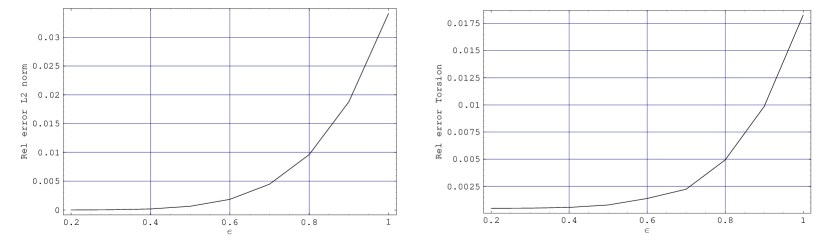
Figure 1. Graphs of the relative errors for the $L^{2}$ norm and the torsion in the case of the folium; the comparison is between the numerical solution obtained by the MFS and the asymptotic expansion given by equations (6.1) and (6.2).

6.2. Lemniscate

We consider the domain $\Omega_{\varepsilon}$ whose boundary is the lemniscate defined by

$$\left(x^{2}+\varepsilon^{-2}y^{2}\right)^{2}=x^{2}-\varepsilon^{-2}y^{2},\quad x>0.$$

The functions $H$, $h_{\pm}$, $d$ and $p$ are given by the formulas

$$H(x)=2h_{+}(x)=2h_{-}(x)=2\left[-\frac{1}{2}-x^{2}+\frac{1}{2}(1+8x^{2})^{1/2}\right]^{1/2},$$

$$d(x)\equiv 0,\quad p=-\frac{1}{2}-x^{2}+\frac{1}{2}(1+8x^{2})^{1/2},\quad\omega=(0,1).$$

Some straightforward calculations give

$$u^{\varepsilon}(x,\xi) =\left(-\frac{1}{2}-x^{2}+\frac{1}{2}(1+8x^{2})^{1/2}-\xi^{2}\right)\varepsilon^{2}+$$

$$+\frac{\left[(1+8x^{2})^{3/2}-2\right]\left(1+2x^{2}-\sqrt{1+8x^{2}}+2\xi^{2}\right)}{\displaystyle 2(1+8x^{2})^{3/2}}\varepsilon^{4}$$

$$+\Bigg{(}4\xi^{4}\frac{32x^{2}-1}{(1+8x^{2})^{7/2}}$$

$$+\xi^{2}\frac{(-512x^{6}-192x^{4}-216x^{2}+7)\sqrt{1+8x^{2}}+256x^{4}+328x^{2}-8}{(1+8x^{2})^{7/2}}$$

$$-\frac{\big{(}1+2x^{2}-\sqrt{1+8x^{2}}\big{)}p_{2}(x)}{2(1+8x^{2})^{7/2}}\Bigg{)}\varepsilon^{6}+\mathcal{O}(\varepsilon^{8}),$$

$$p_{2}(x) :=\sqrt{1+8x^{2}}(512x^{6}+192x^{4}+152x^{2}-5)-128x^{4}-268x^{2}+6.$$

The maximum of $H$ is now situated at $\overline{x}=\sqrt{3}/(2\sqrt{2})$ and using

$$H_{0}=\frac{\sqrt{2}}{2},\quad d_{0}=\operatorname{tr}D_{2}=0,\quad 2\operatorname{tr}P_{2}=-\frac{3}{2},$$

in Theorem 2 then yields

$$\max_{x\in\Omega_{\varepsilon}}u^{\varepsilon}(x)=\frac{\varepsilon^{2}}{8}-\frac{3\varepsilon^{4}}{32}+\mathcal{O}(\varepsilon^{5}).$$

By applying Theorem 3 we arrive at the asymptotics for the torsional rigidity

$$\int_{\Omega_{\varepsilon}}u^{\varepsilon}(x)\,\mathrm{d}x= \frac{3\pi-8}{48}\varepsilon^{3}+\left[\frac{\sqrt{3}}{4}\ln(2+\sqrt{3})-\frac{3\pi}{16}\right]\varepsilon^{5}$$

$$+\left[\frac{13}{18}+\frac{5\pi}{16}-\frac{20\sqrt{3}}{27}\ln(2+\sqrt{3})\right]\varepsilon^{7}+\mathcal{O}(\varepsilon^{9}),$$

where the integrals appearing in the coefficients can be calculated by the Euler substitution

$$\sqrt{1+8x^{2}}=xt+1,\quad x=\frac{2t}{8-t^{2}},\quad t=\frac{\sqrt{1+8x^{2}}-1}{x}.$$

As in the previous example, we show in Figure 2 the relative errors for the $L^{2}$ norm and the torsion in this case. However, comparing the two examples gives that for $\varepsilon$ larger than approximately $0.4$ the errors become much larger than in the case of the folium.

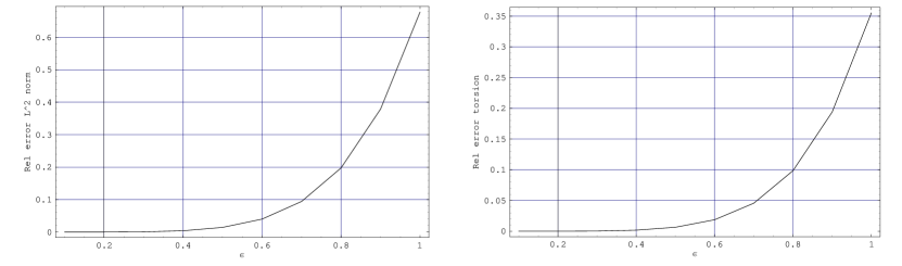
Figure 2. Graphs of the relative errors for the $L^{2}$ norm and the torsion in the case of the lemniscate, with the different quantities computed in a similar way to what was done for the folium.

6.3. Ellipsoids

As mentioned in the Introduction, these are one of the few examples where the explicit solution of the corresponding equation (1.1) is known. More precisely, if we consider ellipsoids defined by

$$E=\left\{x\in\mathbb{R}^{n}:\left(\frac{\displaystyle x_{1}}{\displaystyle a_{1}}\right)^{2}+\dots+\left(\frac{\displaystyle x_{n}}{\displaystyle a_{n}}\right)^{2}=1\right\}$$

we have that the solution of equation (1.1) in this case is given by

$$u(x)=\frac{\displaystyle 1}{\displaystyle\frac{\displaystyle 1}{\displaystyle a_{1}^{2}}+\dots+\frac{\displaystyle 1}{\displaystyle a_{n}^{2}}}\left[1-\left(\frac{\displaystyle x_{1}}{\displaystyle a_{1}}\right)^{2}-\dots-\left(\frac{\displaystyle x_{n}}{\displaystyle a_{n}}\right)^{2}\right]$$

The maximum is thus localized at the origin and is given by

$$M=\frac{\displaystyle 1}{\displaystyle\frac{\displaystyle 1}{\displaystyle a_{1}^{2}}+\dots+\frac{\displaystyle 1}{\displaystyle a_{n}^{2}}}.$$

Let’s assume that $a_{n}$ is the smallest of the $a_{j}$’s, and we thus pick this direction to be that along which we scale the domain. We then have

$$H(x^{\prime})=2h_{+}(x^{\prime})=2h_{-}(x^{\prime})=2a_{n}\left[1-\left(\frac{\displaystyle x_{1}}{\displaystyle a_{1}}\right)^{2}-\dots-\left(\frac{\displaystyle x_{n-1}}{\displaystyle a_{n-1}}\right)^{2}\right]^{1/2},$$

while $d$ vanishes and

$$p(x^{\prime})=a_{n}^{2}\left[1-\left(\frac{\displaystyle x_{1}}{\displaystyle a_{1}}\right)^{2}-\dots-\left(\frac{\displaystyle x_{n-1}}{\displaystyle a_{n-1}}\right)^{2}\right].$$

From this it follows that the maximizer is $\mathcal{O}(\varepsilon^{3})$, while the maximum has the expansion

$$M=a_{n}^{2}\varepsilon^{2}-a_{n}^{4}\displaystyle\sum_{j=1}^{n-1}\frac{\displaystyle 1}{\displaystyle a_{j}^{2}}\varepsilon^{4}+\mathcal{O}(\varepsilon^{6}).$$

A straightforward analysis of the error

$$\mathcal{E}_{M}=\left[\frac{\displaystyle 1}{\displaystyle\frac{\displaystyle 1}{\displaystyle a_{1}^{2}}+\dots+\frac{\displaystyle 1}{\displaystyle\varepsilon^{2}a_{n}^{2}}}-a_{n}^{2}\varepsilon^{2}+a_{n}^{4}\displaystyle\sum_{j=1}^{n-1}\frac{\displaystyle 1}{\displaystyle a_{j}^{2}}\varepsilon^{4}\right]\left(\frac{\displaystyle 1}{\displaystyle\frac{\displaystyle 1}{\displaystyle a_{1}^{2}}+\dots+\frac{\displaystyle 1}{\displaystyle\varepsilon^{2}a_{n}^{2}}}\right)^{-1}$$

yields that this satisfies

$$0\leq\mathcal{E}_{M}\leq\varepsilon^{4}(n-1)^{2},$$

with equality on the right-hand side being achieved for the ball.

For the sake of comparison with the previous two-dimensional examples, we shall now consider the case of the planar disc (in the above notation, $n=2,a_{1}=1,a_{2}=\varepsilon$). In this case the above expressions yield that the relative error of the $L^{2}$ norm and of the torsion are, respectively, $\varepsilon^{12}+\mathcal{O}(\varepsilon^{13})$ and $\varepsilon^{6}+\mathcal{O}(\varepsilon^{7})$. Thus, although the approximation is very good for sufficiently small values of $\varepsilon$, the error does become quite large as $\varepsilon$ reaches one.

References

- [AFR] A. Alabert, M. Farré and R. Roy, Exit times from equilateral triangles, Appl. Math. Optim. 49 (2004), 43-53.
- [BBC] R. Bañuelos, M. van den Berg and T. Carroll, Torsional rigidity and expected lifetime of Brownian motion, J. London Math. Soc. 66 (2002), 499-512.
- [BF1] D. Borisov and P. Freitas, Singular asymptotic expansions for Dirichlet eigenvalues and eigenfunctions of the Laplacian on thin planar domains, Ann. Inst. H. Poincaré Anal. Non Linéaire 26 (2009) 547-560.
- [BF2] D. Borisov and P. Freitas, Asymptotics of Dirichlet eigenvalues and eigenfunctions of the Laplacian on thin domains in , J. Funct. Anal. 258 (2010), 893–912, doi:10.1016/j.jfa.2009.07.014.
- [BEGK] A. Bovier, M. Eckhoff, Gayrard and M. Klein, Metastability in reversible diffusion processes I. Sharp asymptotics for capacities and exit times, J. European Math. Soc. 6 (2004), 399–424.
- [GT] D. Gilbarg and N.S. Trudinger, Elliptic Partial Differential Equations of Second Order, Second Edition. Springer-Verlag, Berlin, 1983.
- [GvH] J. Grasman and O.A. van Herwaarden, Asymptotic methods for the Fokker-Planck equation and the exit problem in applications, Springer Series in Synergetics. Springer-Verlag, Berlin, 1999.
- [GKP] A. Gray, L. Karp and M.A. Pinsky, The mean exit time from a tube in a Riemannian manifold. Probability theory and harmonic analysis (Cleveland, Ohio, 1983), 113–137, Monogr. Textbooks Pure Appl. Math. 98, Dekker, New York, 1986.
- [LU] O. A. Ladyzhenskaya and N. N. Uraltseva, Linear and quasilinear elliptic equations, Academic Press, New York-London, 1968.
- [MP] P. Mörters and Y. Peres, Brownian motion, Cambridge Series in Statistical and Probabilistic Mathematics, V. 30, Cambridge University Press, Cambridge, 2010.
- [N] S. A. Nazarov, Asymptotic analysis of thin plates and rods. V. 1. Reduction of the dimension and integral estimates, Nauchnaya kniga, Novosibirsk, 2002 (in Russian).
- [NT] S. A. Nazarov, J. Taskinen, Asymptotics of the solution to the Neumann problem in a thin domain with sharp edge, J. Math. Sciences 142 (2007), 2630-2644.
- [U] K. Uchiyama, Asymptotic estimates of the distribution of Brwonian hitting time of a disc, J. Theor. Prob. (2010), DOI 10.1007/s10959-010-0305-8.