Core reconstruction in pseudopotential calculations

Abstract

A new method is presented for obtaining all-electron results from a pseudopotential calculation. This is achieved by carrying out a localised calculation in the region of an atomic nucleus using the embedding potential method of Inglesfield [J.Phys. C 14, 3795 (1981)]. In this method the core region is reconstructed, and none of the simplifying approximations (such as spherical symmetry of the charge density/potential or frozen core electrons) that previous solutions to this problem have required are made. The embedding method requires an accurate real space Green function, and an analysis of the errors introduced in constructing this from a set of numerical eigenstates is given. Results are presented for an all-electron reconstruction of bulk aluminium, for both the charge density and the density of states.

I Introduction

Total energy pseudopotential methods have taken pride of place in the first principles simulation of condensed matter in recent years due to their efficient use of computing resources and their suitability for structural optimisation payne92 . However, the charge density resulting from a pseudopotential calculation is incorrect in the region near the atomic nuclei - it does not include core states, and the valence states have the wrong structure. In order to obtain accurate values for any quantity that depends on the true charge density, such as hyperfine interactions or X-ray structure factors, we must obtain the correct electron charge density from the pseudopotential calculation. Other methods are available that calculate the states of all the electrons in the system (Full-potential Linear Augmented Plane Wave (FLAPW)hill98 , Projector Augmented Plane Wave (PAW)blochl94 , Linear Muffin Tin Orbital (LMTO)turzhevsky94 , KKR Green function huhne98 and Tight Binding goringe97 ), but these methods tend to be more computationally expensive, not as well suited to structural optimisation, or are less accurate than pseudopotential methods.

In view of this it is desirable to extend the pseudopotential method by adding an extra step after the pseudo-system has been solved, ie to choose an atom for which we require the core and correct valence states, and reconstruct these correct states. It would be hoped that solving for one atom with different boundary conditions on a sphere surrounding it would be fairly straightforward. However, a number of difficulties quickly present themselves. The purpose of this paper is to describe and validate a new procedure for carrying out this core reconstruction that makes essentially the same physical approximations as the FLAPW method, and so can be expected to provide the same accuracy.

This problem has been addressed by several previous workers. In their paper Gardner and Holzworth gardner86 reconstruct the correct states for isolated Si and Ru atoms from the pseudo-atom, by applying direct integration, effectively ‘inverting’ the pseudopotential. They obtain good results, showing that this reconstruction approach is at least possible. However, reconstructing the states of an atom in a lattice is considerably more complex. For this case the valence states form a continuum, so the reconstruction must be fitted into the band structure of the lattice, and in addition to this the potential is not spherically symmetric. Vackář and Šimu̇nek vackar94 describe a method for reconstructing the states for a pseudo-atom within a lattice. Their method relies on direct integration and assumes the charge density, boundary conditions and self-consistent potential are spherically symmetric, although the core states are allowed to relax. The errors in the resulting eigenfunctions are fairly large, although they do obtain the correct nodal form for the eigenstates. Kuzmiak et alkuzmiak91 perform a pseudopotential calculation, and orthogonalise the resultant pseudo-states to the original core states. This would work for the original formulation of pseudopotential methods, where the pseudopotential is defined in this way, but for modern norm-conserving pseudopotentials this does not give the correct solution to the problem and the errors present are difficult to control or even quantify. The most complete solution to the problem presented so far is that due to Meyer et al meyer95 . In their method the correct states are reconstructed by direct integration. In order to decouple the radial wave equations for the reconstruction calculation they make the assumption of spherical symmetry of the self consistent potential, but asymmetric boundary conditions for the valence states are allowed. Within their scheme the core is still frozen.

In this paper a new method for performing this kind of core reconstruction is described that does not make any of the assumptions of previous approaches. The method presented here follows a different path to achieving the reconstruction, does not require spherical averaging of the self-consistent potential, provides an aspherical charge density, and does not assume a frozen core. The first step is to carry out a plane-wave pseudopotential calculation for the system of interest, and construct the single particle Green function for the valence electrons present in this system. This Green function is then used to create an embedding potential, as described by Inglesfield inglesfield81 . An all-electron localised atomic calculation is then carried out in a space containing the core region of the atom of interest, with the embedding potential taking into account the rest of the atoms in the lattice. Effectively the system that is solved for is one all-electron atom in a lattice of pseudo-atoms. This approach preserves the full generality and flexibility of the pseudopotential method. In addition, the all-electron calculation is carried out only for the atom(s) of interest, so computational effort can be applied sparingly.

In the next section a brief description is given of the embedding approach, how it is applied in this case, and how it relies on an accurate knowledge of the Green function for the substrate system. Appendix A gives a more complete description of the method and its properties. In section III we describe how the spectral representation can be efficiently applied in order to construct an accurate Green function, and how the incompleteness of the available set of states introduces a significant error that must be corrected. Combining the results of these two sections we then obtain the embedding potential from the Green function and perform a localised calculation using the embedding terms to take into account the rest of the lattice, as described in section IV. Section V gives the results of a reconstruction carried out for bulk FCC aluminium, and the convergence of the method is discussed. Rydberg atomic units are used throughout the paper.

II Embedding

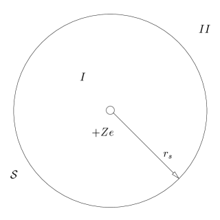
Figure 1: Geometry of embedding calculation. Region $II$ is the substrate region, region $I$ is the embedded region, and the all-electron states are reconstructed from a knowledge of the pseudo-states on the surface $\mathcal{S}$.

An embedding method can be thought of as solving for a system in a sub-domain of space, denoted region $I$ in what follows, where the influence of the system outside of this sub-domain (region $II$) is taken into account from a previous solution, and is not recalculated. This is shown in Fig. 1 for the core reconstruction case considered here. The embedding surface, $\mathcal{S}$, separates regions $I$ and $II$. Region $I$ is a sphere of radius $r_{s}$ enclosing the core region of the atom where the pseudo-states are incorrect and region $II$ is the remainder of the lattice of pseudo-atoms. It is implicitly assumed throughout this work that norm-conserving pseudopotentials are used, so that wavefunctions between core regions are correct. The embedding surface $\mathcal{S}$ is assumed to be in such a region; it follows that core regions do not overlap, hence $r_{s}>r_{c}$ where $r_{c}$ is the largest pseudopotential core radius.

Using Inglesfield’s method inglesfield81 an ‘embedding potential’ is obtained from the substrate system, and added to the Hamiltonian for the embedded region. This embedding potential ensures that the states of the system in the embedded region satisfy the correct boundary conditions. Inglesfield’s method has the advantage that it requires knowledge of the properties of the substrate system only on the surface separating the embedded and substrate regions. In appendix A a brief description of the derivation of the embedding method is given, followed by two expressions for the embedding potential in terms of the Green function for the substrate system, one of which has not appeared in the literature before.

Within a continuum the Hamiltonian of the embedded system takes the form

$$H_{emb}(E)=H_{I}+\delta({\mathbf{r}}_{s}-{\mathbf{r}})\left[\frac{\partial}{\partial n_{s}}-\Gamma({\mathbf{r}}_{s},{\mathbf{r}}^{\prime}_{s};E)\right]$$ (1)

where $H_{emb}(E)$ is the embedded Hamiltonian that yields the states with correct boundary conditions, $H_{I}$ is the normal Hamiltonian for the embedded region, and $\Gamma$ is the embedding potential. It should be understood at this point that $\Gamma({\mathbf{r}}_{s},{\mathbf{r}}^{\prime}_{s};E)$ acting on a function denotes the integration over the surface $\mathcal{S}$, as described in appendix A. Equation (1), when solved in region $I$, will give the correct solution for the system represented by regions $I$ and $II$, with region $II$ represented entirely through the embedding potential term. The embedding potential required in equation (Eq. (1)) is given by the operator

$$\Gamma=-{\mathcal{G}}^{-1}.\left({\mathcal{I}}-\frac{\partial{\mathcal{G}}}{\partial n_{s}^{\prime}}\right)$$ (2)

where $\mathcal{G}$ is the matrix representation of the Green function on the surface $\mathcal{S}$ in terms of a set of basis functions orthonormal over the surface, and the derivative is the normal derivative of $\mathcal{G}$ outward from the surface and with respect to the second spatial variable of the Green function. A derivation of Eqs. (1) and (2) is given in appendix A.

III Green Function and Embedding potential

The embedding method of the previous section is to be applied with the substrate system represented by the results of a plane-wave pseudopotential calculation, hence the Green function on the embedding surface must be obtained from the Bloch states expanded in plane-waves. The natural way of constructing this Green function is via the spectral representation, and a finding good approximation to this spectral representation is the concern of this section.

For the periodic system the states are characterised by two quantum numbers, the discrete band index $n$ and the continuous crystal momentum $\mathbf{k}$, so the spectral representation takes the form

$$G({\mathbf{r}},{\mathbf{r}}^{\prime};E)=\sum_{n}\int_{BZ}\frac{\Psi_{\mathbf{k}}^{n}({\mathbf{r}})\Psi^{n*}_{\mathbf{k}}({\mathbf{r}}^{\prime})}{E_{n}({\mathbf{k}})-E}d^{3}{\mathbf{k}}$$ (3)

where $\Psi_{\mathbf{k}}^{n}({\mathbf{r}})$ is a Bloch state, $E_{n}({\mathbf{k}})$ is its eigenenergy and $E$ is complex in general. For the periodic lattice both the total number of states and the number of states within a given energy interval (in a band) is infinite, but any numerical calculation can only provide states at a finite number of ${\mathbf{k}}$-points, and for a finite number of bands payne92 . In view of these restrictions the approximation of the spectral representation falls naturally into two parts - approximating the Brillouin zone integral from a finite number of $\mathbf{k}$-points, and approximating the infinite band sum. It should be noted that although it is well established that Green function methods and the spectral representation can be defined within a limited basis set williams82 , the embedding method cannot be applied in this way since it relies on the properties of the Green function in real space fisher88 .

III.1 The Spectral function

The simplest way to apply the defining equations for the embedding potential is to expand the Green function in a set of basis functions that are orthogonal over the embedding surface. For the core reconstruction considered here the embedding surface is a sphere centred on the atomic site of interest, hence a natural set of basis states are the spherical harmonics. First the Kohn-Sham wavefunctions are expanded on the surface $\mathcal{S}$,

$$\Psi^{n}_{\mathbf{k}}({\mathbf{r}}_{s})=\sum_{\mathbf{g}}C_{\mathbf{g}}^{n}({\mathbf{k}})e^{i({\mathbf{k}}+{\mathbf{g}}).{\mathbf{r}}_{s}}=\sum_{L}\alpha^{(n)}_{L}({\mathbf{k}})Y_{L}(\hat{\mathbf{r}})$$ (4)

where $L=(lm)$, the combined index of the spherical harmonic $Y_{L}$, and $C_{\mathbf{g}}^{n}({\mathbf{k}})$ are the expansion coefficients of the eigenstates in the plane-wave representation. The expansion coefficients $\alpha^{(n)}_{L}({\mathbf{k}})$ can be found using the identity morse53

$$e^{i{\mathbf{q}}.{\mathbf{r}}}=4\pi\sum_{L}i^{l}j_{l}(qr)Y_{L}^{*}(\hat{\mathbf{q}})Y_{L}(\hat{{\mathbf{r}}})$$ (5)

hence

$$\alpha^{(n)}_{L}({\mathbf{k}})=4\pi i^{l}\sum_{\mathbf{g}}j_{l}(|{\mathbf{k}}+{\mathbf{g}}|r_{s})Y^{*}_{L}(\widehat{{\mathbf{k}}+{\mathbf{g}}})C_{\mathbf{g}}^{n}({\mathbf{k}}).$$ (6)

From these a ‘spectral function’ ${\mathcal{F}}_{LL^{\prime}}(E)=\frac{1}{\pi}\text{Im }[{\mathcal{G}}_{LL^{\prime}}(E)]$ can be defined, where ${\mathcal{G}}_{LL^{\prime}}(E)$ are the expansion coefficients for the Green function. This spectral function is given by the equation

$${\mathcal{F}}_{LL^{\prime}}(E)=\sum_{n}\int_{BZ}d^{3}{\mathbf{k}}\ \alpha^{(n)}_{L}({\mathbf{k}})\alpha^{(n)*}_{L^{\prime}}({\mathbf{k}})\delta(E-E_{n}({\mathbf{k}}))$$ (7)

and is related to the Green function by the convolution integral

$${\mathcal{G}}_{LL^{\prime}}(E)=\int_{-\infty}^{\infty}dE^{\prime}\ \frac{{\mathcal{F}}_{LL^{\prime}}(E^{\prime})}{E^{\prime}-E}.$$ (8)

In Eq. (7) the integral on the right hand side reduces to the surface integral

$${\mathcal{F}}_{LL^{\prime}}(E)=\sum_{n}\int_{E=E_{n}({\mathbf{k}})}\frac{\alpha^{(n)}_{L}({\mathbf{k}})\alpha^{(n)*}_{L^{\prime}}({\mathbf{k}})}{|\nabla_{\mathbf{k}}E|}dS$$ (9)

due to the delta function, hence evaluation of the spectral representation reduces to the evaluation of a surface integral in ${\mathbf{k}}$-space and a singular convolution integral in energy space. The surface integral is carried out using the linear analytic tetrahedron method lehmann72 ; jepson71 ; macdonald79 ; rath75 ; kaprzyk86 , which results in a spectral function that has the correct analytic structure in that it is continuous in energy. Only the irreducible wedge need be sampled with the symmetry of the crystal used to complete the rest of the integral trail98 .

In order to evaluate Eq. (8) the singular integral itself must be approximated from a sampling of the function at a finite number of energy values. Here the spectral function is interpolated between consecutive energy values, and the contribution to the integral from each of these ranges calculated. We use a polynomial interpolation, so the integrals can be evaluated analytically davis67 . This results in an approximation to the Green function that can be evaluated for complex $E$ and which has the analytic properties appropriate for a continuum of states; it is essentially a generalisation of the approach used by Kuzmiak et al kuzmiak91 to complex energies. An alternative application of the linear analytic tetrahedron method to the calculation of Green functions is given Lambin and Vigneron lambin84 where Eq. (3) is evaluated for each tetrahedron analytically, within the linear interpolation scheme. Although this approach is more direct and introduces none of the errors due to approximating Eq. (8), it requires the interpolation to be applied to all tetrahedra, whereas the surface integral in Eq. (9) requires only a sub-set of tetrahedra to be considered for each energy. In addition to this the surface integral and convolution route allows a greater flexibility in the degree of approximation applied, as discussed below.

III.2 Completing the Incomplete Set of States

So far the evaluation of the Green function takes into account the continuum nature of the band states, but for the spectral representation to describe a real space Green function the set of states used in Eq. (3) must be complete. We have found that in order to obtain accurate Green functions using the spectral representation, we must include the complete set of $n_{\mathbf{g}}$ states associated with the plane-wave basis set (for further discussion see Trailtrail98 ). $n_{\mathbf{g}}$ is the number of plane-waves in the basis set, determined by the plane-wave energy cut-off, and these states will be obtained by direct matrix diagonalisation of the Kohn-Sham Hamiltonian. This set of states is still not complete in real space, hence we must consider the errors introduced by not including the energy bands that are not available in a finite plane-wave calculation. In what follows we refer to the spectral representation that includes only the $n_{\mathbf{g}}$ lowest energy bands as the incomplete spectral representation. It is important to realise that we mean the states are incomplete in real space, they are, of course, complete in the sub-space spanned by the plane-wave basis set.

It is not immediately apparent that this incompleteness will have a significant effect, and it could be hoped that the ‘missing’ high energy states are so far above the energies of interest (ie at or below the Fermi energy) that any error introduced by their absence will be negligible. This is only partly true, and the properties of the error introduced by incompleteness are derived in appendix B for a free electron gas. Correcting for this incompleteness not only speeds convergence with respect to $n_{\mathbf{g}}$, it also ensures that the approximation of the Green function has the correct analytic form. We follow James and Woodley james96 and approximate the high energy states ‘missing’ from the incomplete spectral representation by free electron states. The plane-wave basis set used to represent the lowest $n_{\mathbf{g}}$ bands is described by $|{\mathbf{g}}|^{2}<E_{max}$, where ${\mathbf{g}}$ are reciprocal lattice vectors and $E_{max}$ is the standard plane-wave cut-off energy. Consequently, the free electron states required to ‘top up’ the incomplete spectral representation are those described in the reduced zone scheme by $|{\mathbf{g}}|^{2}\geq E_{max}$ and ${\mathbf{k}}$ in the first Brillouin zone.

In order to calculate the required correction we calculate an incomplete spectral representation for free electrons with exactly the same basis as for the pseudopotential states, and subtract this from the analytic free electron Green function. This yields the approximation

$${\mathcal{G}}\approx{\mathcal{G}}^{pseudo}_{E_{max}}-{\mathcal{G}}^{free}_{E_{max}}+{\mathcal{G}}^{free}_{\infty}$$ (10)

where the first term on the right hand side is the incomplete spectral representation of the pseudo-states, the second is the incomplete spectral representation of free electron states and the final term the complete spectral representation for free electron states (ie the analytic free electron Green function). In terms of the spectral function, ${\mathcal{F}}$, and the convolution integral used to transform this into the spectral representation, Eq. (8) becomes

$${\mathcal{G}}_{LL^{\prime}}(E)=\int\frac{{\mathcal{F}}^{pseudo}_{LL^{\prime}}(E^{\prime})-{\mathcal{F}}^{free}_{LL^{\prime}}(E^{\prime})}{E^{\prime}-E}dE^{\prime}+{\mathcal{G}}^{\infty}_{LL^{\prime}}(E)$$ (11)

where ${\mathcal{G}}$ is now a Green function with the correct analytic form, $E$ is complex and $E^{\prime}$ is real. ${\mathcal{F}}^{pseudo}$ and ${\mathcal{F}}^{free}$ are the spectral functions associated with the pseudo-states and the free space states respectively, calculated with $n_{\mathbf{g}}$ basis functions. The last term, ${\mathcal{G}}^{\infty}$, is the analytic free space Green function given by morse53 ; abramowitz64

$${\mathcal{G}}^{\infty}_{LL^{\prime}}=ikj_{l}(kr_{s})h_{l}(kr_{s})\delta_{ll^{\prime}}$$ (12)

where $j_{l}$ is the spherical Bessel function of the first kind, $h_{l}$ is the spherical Hankel function of the first kind and $E=k^{2}+V_{0}$, where $V_{0}$ is the average potential within the unit cell. In practice the specific value of $V_{0}$ is not critical since the error term varies only slowly with the Green function energy, as discussed in appendix B. The normal derivative of the Green function can be obtained by taking the radial derivative of the Green function, and Eq. (2) directly applied to give the embedding potential (a factor of $\frac{1}{r_{s}^{2}}$ must be included to normalise the spherical harmonics over the embedding sphere). Eq. (38) was not used due to problems with small errors in the Green function introducing anomalous poles at the bottom of the lowest band.

IV Embedding Calculation

In this section we describe the all-electron calculation carried out in the region near the nucleus, using the embedding potential described above. The normal density functional framework is used, with the Kohn-Sham Hamiltonian extended by the addition of the embedding terms. Since these extra terms are functions of energy the eigenvalue solution of the Hamiltonian is not simple, hence the charge density is obtained directly from the Hamiltonian via the Green function method as described by Williams et al williams82 . The method employed in the all-electron calculation is similar to that used by other workers (eg Trioni et al trioni96 ), but generalised so as not to require any particular symmetry of the charge density or self-consistent potential, and to include core electrons.

IV.1 The Embedded Hamiltonian

Each basis function is a product of a radial function and a spherical harmonic, with the radial part defined as an augmented plane-wave for $r<s$ (region $B$) and a spherical Bessel function for $s<r<r_{s}$ (region $A$), where $s$ is a parameter of the calculation. These are chosen since Linearised Augmented Plane Waves (LAPW) orbitals describe the all-electron valence states well near the nucleus, and in the region nearer the embedding radius the spherical Bessel functions provide the flexibility required to satisfy the boundary conditions.

The basis functions in region $B$ are found by solving the Dirac equation using numerical integration in the spherical part of the Kohn-Sham potential. The method used is that described by Koelling and Harmon koelling77 , where the Dirac equation is approximated in the form of a Schrödinger equation which does not include spin-orbit interaction but takes other relativistic effects into account. A solution is found at a fixed ‘pivot’ energy, $E_{p}$, and the resultant radial functions are denoted $u_{l}(r)$. The energy derivative of these functions are also obtained and orthogonalised to the associated $u_{l}(r)$, and these orthogonalised energy derivatives are denoted $\dot{u}_{l}(r)$ (see Krasovskii krasovskii97 , or Takeda and Kübler takeda79 ). In $A$ the radial basis functions used are spherical Bessel functions of the first kind, defined as $j_{l}(g_{i}r)$ where $g_{i}=\frac{\pi i}{d}$. The index $i$ is chosen to take integer values, to give a set of functions, and $d$ is a parameter of the calculation (larger than $r_{s}$ to allow sufficient flexibility for the basis function to satisfy arbitrary boundary conditions). The radial parts of the basis functions, $\chi_{il}(r)$ are therefore

$$\chi_{il}(r)=\left\{\begin{array}[]{ll}a_{il}u_{l}(r)+b_{il}\dot{u}_{l}(r)&0\leq r\leq s\\ j_{l}(g_{i}r)&s<r\leq r_{s}\ .\end{array}\right.$$ (13)

Parameters $a_{il}$ and $b_{il}$ are chosen to ensure $\chi_{il}$ is continuous in amplitude and derivative at the $AB$ boundary. Typically $r_{s}$ is chosen to be half the distance between nearest neighbour atoms in the lattice, $s\sim 0.9r_{s}$ and $d\sim 2r_{s}$ to give a good description of the valence electrons. For $i$ the range $1\ldots 4$ is typical.

The embedded Hamiltonian matrix is then expanded in terms of these basis functions, for a Kohn-Sham potential given by

$$V({\mathbf{r}})=\sum_{L}V_{L}(r)Y_{L}(\hat{\mathbf{r}})$$ (14)

where $L=(lm)$, the index of the spherical harmonic. We write Hamiltonian matrix, ${\mathbf{H}}_{emb}$, as the sum of $3$ parts,

$${\mathbf{H}}_{emb}={\mathbf{H}}^{A}+{\mathbf{H}}^{B}+{\mathbf{\Sigma}}$$ (15)

with ${\mathbf{H}}^{A}$ the contribution from region $A$, ${\mathbf{H}}^{B}$ the contribution from region $B$, and ${\mathbf{\Sigma}}$ the contribution from the embedding terms at the surface ${\mathcal{S}}$. Integrating over region $A$ results in

$$H^{A}_{iL,jL^{\prime}}=g_{j}^{2}\int_{s}^{r_{s}}r^{2}dr\left[j_{l}(g_{i}r)j_{l}(g_{j}r)\right]\delta_{LL^{\prime}}$$

$$+\sum_{L^{\prime\prime}}S^{L}_{L^{\prime}L^{\prime\prime}}\int_{s}^{r_{s}}r^{2}dr\left[j_{l}(g_{i}r)V_{L^{\prime\prime}}(r)j_{l^{\prime}}(g_{j}r)\right],$$ (16)

where $S^{L}_{L^{\prime}L^{\prime\prime}}=\int Y_{L}^{*}Y_{L^{\prime}}Y_{L^{\prime\prime}}d\Omega$ are Gaunt coefficients. For region $B$ we find a sum of spherical and aspherical terms

$$H^{B}_{iL,jL^{\prime}}= \left[a_{il}a_{jl}E_{p}\langle u_{l}\mid u_{l}\rangle\right.$$ (17)

$$\left.+a_{il}b_{jl}\langle u_{l}\mid\dot{u}_{l}\rangle+b_{il}b_{jl}E_{p}\langle\dot{u}_{l}\mid\dot{u}_{l}\rangle\right]\delta_{LL^{\prime}}$$

$$+\sum_{L^{\prime\prime}\neq 0}S^{L}_{L^{\prime}L^{\prime\prime}}\int_{0}^{s}r^{2}dr\chi_{il}(r)V_{L^{\prime\prime}}(r)\chi_{jl^{\prime}}(r)$$

where $E_{p}$ is the ‘pivot’ energy at which $u_{l}(r)$ is calculated, and the bra-ket’s denote integration over region $B$ only. The integrals in the above expressions are carried out analytically or numerically as appropriate. Taking the normal derivative and embedding potential terms in Eq. (1) we obtain the contribution from the embedding terms, ${\mathbf{\Sigma}}$, as

$$\Sigma_{iL,jL^{\prime}}= j_{l}(g_{i}r_{s})\Gamma_{LL^{\prime}}(E)j_{l^{\prime}}(g_{j}r_{s})$$ (18)

$$+g_{j}j_{l}(g_{i}r_{s})j^{\prime}_{l^{\prime}}(g_{j}r_{s})\delta_{L,L^{\prime}}.$$

In addition to the Hamiltonian matrix the overlap matrix of the basis functions, $\mathbf{O}$, is also required. This is given by

$$O_{iL,jL^{\prime}}=\delta_{LL^{\prime}}\int_{s}^{r_{s}}j_{l}(g_{i}r)j_{l}(g_{j}r)r^{2}dr$$

$$+\left[a_{il}a_{jl}\langle u_{l}\mid u_{l}\rangle+b_{il}b_{jl}\langle\dot{u}_{l}\mid\dot{u}_{l}\rangle\right]\delta_{LL^{\prime}}$$ (19)

where the first integral on the right hand side can be performed analytically abramowitz64 and the second numerically.

IV.2 The Embedded Green function and Charge Density

The Green function of the embedded system is obtained directly by matrix inversion,

$${\mathbf{G}}(E)=\left({\mathbf{H}}_{emb}(E)-E{\mathbf{O}}\right)^{-1},$$ (20)

where ${\mathbf{H}}_{emb}$ is the embedded Hamiltonian described above. To obtain the local density of states, $n({\mathbf{r}};E)$, we apply the identity economou90

$$n({\mathbf{r}};E)=\frac{1}{\pi}\text{Im }G({\mathbf{r}},{\mathbf{r}};E).$$ (21)

By filling all states to the Fermi energy (which is obtained from the original pseudopotential calculation using the linear analytic tetrahedron method) we can obtain the valence charge density. Unfortunately the number of points required to evaluate the charge density by integrating the local density of states is fairly high, due to its fine structure. This can be avoided be taking advantage of Cauchy’s theorem williams82 ; morse53 and the analytic properties of the Green function. We choose a contour $C$ from some energy below the lowest eigenvalue, following a half circle into the positive complex plane and terminating on the real axis at the Fermi energy, so the charge density expanded in spherical harmonics is given by

$$\rho^{val}_{L^{\prime\prime}}(r)= \frac{1}{2\pi}\sum_{ijLL^{\prime}}\chi_{il}(r)\chi_{jl^{\prime}}(r)$$ (22)

$$\times\int_{C}\left(G_{iLjL^{\prime}}S^{L^{\prime}}_{LL^{\prime\prime}}-G^{*}_{iLjL^{\prime}}S^{L}_{L^{\prime}L^{\prime\prime}}\right)$$

where the $G_{iLjL^{\prime}}$ are evaluated at the complex energies on the contour. In this equation $S^{L}_{L^{\prime}L^{\prime\prime}}$ is a Gaunt coefficient, and is zero for $l^{\prime\prime}>2l$ or $2l^{\prime}$, so a $l_{max}\times l_{max}$ Hamiltonian matrix will result in a charge density containing components $l\leq 2l_{max}$. It is due to the basis functions being complex that this expression does not simply involve the imaginary part of the Green function matrix. As the imaginary part of the energy increases the Green function becomes smoother and more featureless, hence a more sparse sampling is sufficient to approximate this integral accurately. Gaussian integration press94 is used to perform the integral along contour $C$, and converged integrals are typically obtained for around $16$ points on the contour.

The core states could be obtained by finding the discrete states of the embedded Hamiltonian, but this would be cumbersome (see appendix A). Core states are therefore obtained using the Kohn-Sham potential within the embedding sphere, and a constant potential outside of the sphere. This gives accurate results as the core states are strongly localised within the core region, so the potential outside of the embedding sphere is largely irrelevant. Only the spherically symmetric part of the potential is used to obtain the states, and the constant potential outside the sphere is taken to be continuous with the spherical part. This spherically symmetric approximation has been used by many workers (eg Blaha et al blaha88 ; Methfessel and Frota-Pessô methfessel90 ), and can easily be extended to included aspherical effects perturbatively as described by Ehmann and Fähnle ehmann97 , Sternheimer sternheimer86 and Lauer et al lauer79 . To obtain the core charge density a fully relativistic treatment is used, solving the Dirac equation within the embedding region.

This approach allows the construction of core-states that are self-consistent within the embedded system, however the influence of core relaxation on the substrate system (and so on the embedding potential) is not considered. Essentially we are assuming that the original pseudopotential approximation is valid, and that the valence pseudo-states are accurate outside of the core region. In order to go beyond this assumption it should be possible to obtain a new pseudopotential from the embedded core states and to iterate to full self-consistency, but this has not been implemented. Similar considerations are discussed by Blöchl blochl94 . It should be noted that for the embedding method applied here the core states are truly localised, since we are embedding an all-electron atom at one site within a lattice of pseudo-atoms.

IV.3 Self Consistency

The Kohn-Sham potential, $V^{KS}({\mathbf{r}})$, is calculated from the total charge density via the Local Density Approximation (LDA), and takes the form

$$V^{KS}_{L}(r)=V^{Nuc}_{L}(r)+V^{Hart}_{L}(r)+V^{XC}_{L}(r),$$ (23)

a sum of the nuclear potential, the Hartree potential, and the exchange-correlation potential respectively. The nuclear potential is assumed to be that of a point charge centred at the nucleus, and the Hartree potential,

$$V^{Hart}_{L}(r)= \frac{4\pi}{2l+1}\frac{1}{r^{l+1}}\int_{0}^{r}\left[r^{\prime l}\rho_{L}(r^{\prime})\right]r^{\prime 2}dr^{\prime}$$ (24)

$$+\frac{4\pi}{2l+1}r^{l}\int_{r}^{r_{s}}\left[\frac{1}{r^{\prime l+1}}\rho_{L}(r^{\prime})\right]r^{\prime 2}dr^{\prime}$$

$$+a_{L}r^{l},$$

is obtained from Poisson’s equation. The constants $a_{L}$ are defined by the boundary condition that the Kohn-Sham potential, $V^{KS}_{L}(r)$, be equal to the self-consistent potential of the original pseudopotential calculation on the embedding sphere.

The LDA is used to obtain the exchange-correlation potential from the charge density using the Perdew and Zunger parameterisation perdew81 of the results of Ceperly and Alder ceperly80 (this was also used in the original pseudopotential calculation). $V^{XC}({\mathbf{r}})$ is a non-linear function of the charge density, so $V^{XC}_{L}(r)$ cannot be directly obtained from $\rho_{L}(r)$. However, deviations from a spherical density are expected to be small, so we expand the exchange-correlation potential as a Taylor series

$$V^{XC}(\rho)=V^{XC}(\rho_{0})+\left.\frac{\partial V^{XC}}{\partial\rho}\right|_{\rho_{0}}(\rho-\rho_{0})+\cdots$$ (25)

with $\rho_{0}$ the spherical part of the charge density. A truncation to linear order is sufficiently accurate (the quadratic terms are negligible for the systems considered to date) and can be applied directly. Convergence to self-consistency is achieved, with instabilities controlled and convergence speed increased by applying Broyden mixing broyden65 ; johnson88 .

V Results

In order to test the effectiveness of the embedding method for core reconstruction we examine aluminium in the FCC structure. We begin by giving an example of the calculated embedding potentials, and some concrete evidence that the approximations made can give an accurate embedding potential. The initial self-consistent plane-wave calculation is carried using the LDA, a plane-wave cut-off of $400$ eV and 60 $\mathbf{k}$-points within the FCC irreducible wedge. These parameters are more than adequate to obtain effectively perfect convergence, so we can attribute any errors in the reconstruction to the embedding method. A Kerker kerker80 pseudopotential is used with a core radius $r_{c}=2.19\ au$, small enough for the core regions not to overlap. The resulting self-consistent potential is then used to obtain the full set of eigenstates by matrix diagonalisation for a plane-wave basis set $|{\mathbf{g}}|^{2}<E_{max}$, and at the $\mathbf{k}$-points required to carry out the Brillouin zone integral using the linear analytic tetrahedron method. These states are then used to construct the embedding potential, with the embedded sphere taken as the ‘touching sphere’ radius, $r_{s}=2.705\ au$. The convergence behaviour of the embedding potential depends on the number of plane-waves in the basis, $n_{\mathbf{g}}$, the number of ${\mathbf{k}}$-points in the irreducible wedge of the FCC Brillouin zone, $n_{\mathbf{k}}$, and the spacing of energy points ($\Delta E$) used to sample the spectral function, ${\mathcal{F}}$ (see Eq. (8)).

Figure 2: (a) Real part, (b) imaginary part of aluminium embedding potential matrix element, $\Gamma_{(10,10)}$, for $n_{\mathbf{k}}=240$ (solid line, for clarity shown offset by $-0.02$ for both real and imaginary parts) and $n_{\mathbf{k}}=505$ (dashed line). The difference is also shown as the solid line near $\Gamma_{(10,10)}=0.0$.

Fig. 2 shows the $\Gamma_{(10,10)}$ matrix element for the imaginary part of the energy equal to $0.1$ eV. Results are shown for $E_{max}=200$ eV and $\Delta E=0.3$ eV with linear interpolation of the spectral function, and for both $240$ and $505$ $\mathbf{k}$-points in the irreducible wedge of the Brillouin zone. There is very little discernable difference between the two results, $<0.002$ for both the real and imaginary parts, hence we consider $505$ $\mathbf{k}$-points as effectively converged. Using $89$ $\mathbf{k}$-points results in larger errors ($<0.01$), but was found to be adequate for performing an accurate reconstruction, as discussed below. The difference between $E_{max}=200$ and $400$ eV is even smaller ($<0.001$), and comparing $\Delta E=0.3$ eV to $0.1$ eV again gives a difference of $<0.001$. The other matrix elements show a similar convergence behaviour. Embedding potentials for use in the reconstructions were therefore calculated with $E_{max}=200$ eV, $\Delta E=0.3$ eV and $240$ $\mathbf{k}$-points, for energies required on the contour of integration (Eq. (22)). Reconstructions were performed for $l_{max}=6$, $d=4.0$, $4$ Bessel functions in the basis (Eq. (13)), and 16 points along the contour of integration. These provided the total charge density within the radius $r_{s}$, the density of states within the embedded region, the self consistent potential and the core eigenstates.

V.1 Embedding with a Pseudopotential

Before reconstructing the all-electron charge density, we carry out a reconstruction in which no core states are included and the core and nucleus are described by a pseudopotential, the same Kerker pseudopotential used in the original plane-wave calculations. This provides a stringent test of the accuracy and reliability of the entire embedding approach, since for a successful implementation the resulting valence charge density should be the same as the original plane-wave charge density throughout the embedding sphere. The Fermi energy used within the reconstruction is obtained from the original plane-wave calculation, hence the total valence charge within the embedding sphere will be different from the plane-wave calculation, and the size of this difference provides a first indication of how accurate the reconstruction is. The original plane-wave calculation has $2.298$ electrons within the embedding sphere, whereas the reconstruction gives $2.300$ - an error of $0.08$ %. This close agreement suggests a successful reconstruction, however this is a fairly gross measure of success since it takes no account of the structure of the electron states within the embedding sphere and compares only the spherical part of the charge density.

	range	peak $(\times 10^{-4}e\textrm{ }au^{-3})$	$R(\%)$
Pseudo	$r<r_{s}$	-5.56	0.49
Pseudo	$r_{c}<r<r_{s}$	-5.56	0.48
All-electron	$r_{c}<r<r_{s}$	-5.47	0.46

Table 1: Errors in charge density for each reconstruction. Pseudo refers to the reconstruction performed using a pseudopotential to represent core states, and All-electron refers to the full all-electron reconstruction. The pseudopotential core radius is $r_{c}=2.19\ au$, and the embedding sphere radius is $r_{s}=2.705\ au$.

A more demanding measure of the accuracy of the reconstruction is to compare the charge density and/or self consistent potential of the original pseudopotential calculation with the reconstruction. The error in the charge density is quantified as the peak error and the $R$ factor press94 defined as

$$R=\int|\rho^{recon}({\mathbf{r}})-\rho^{pseud}({\mathbf{r}})|d^{3}{\mathbf{r}}/\int|\rho^{pseud}({\mathbf{r}})|d^{3}{\mathbf{r}},$$ (26)

and the errors over the whole embedding region are given in Table 1. We also give the error within the shell between the core radius of the pseudopotential and the embedding sphere, which will allow comparison with the all-electron results.

Figure 3: (a) Contours of constant valence charge density in the {100} plane for the original plane-wave (dashed line) and reconstructed pseudopotential (solid line) results. The reconstructed atom is at the centre and the square just encloses the embedding sphere. Contour levels are $0.01$, $0.02$, $0.025$, $0.030$ and $0.032$ $e\textrm{ }au^{-3}$, chosen to emphasise the differences between the original and reconstructed charge densities. (b) Valence charge density along a line in the [011] direction, with the reconstructed atom at the origin. Original plane-wave (dotted line) and reconstructed all-electron results (solid line) are shown. The vertical dashed lines are at the core radius of the pseudopotential.

Fig. 3a shows a contour plot of $\rho({\mathbf{r}})$, for both the original plane-wave and reconstructed charge density. These are taken in the $\{100\}$ plane, with the embedded atom at the centre and the square shown just enclosing the embedding sphere. There is excellent agreement between the original and reconstructed densities, again demonstrating a successful reconstruction.

V.2 The Reconstructed All-electron Charge Density

The total valence charge within the embedding sphere is $2.299$ electrons for the all-electron reconstruction, which again agrees very well with the original plane-wave result. As above we also compare the charge density of the original pseudopotential calculation with the reconstruction. For a successful reconstruction, the original pseudopotential charge density should agree with the reconstructed charge density for $r_{c}<r<r_{s}$. Fig. 3b shows $\rho^{val}({\mathbf{r}})$ along a line in the $[011]$ direction for both the original plane-wave and all-electron reconstruction calculations, with the reconstructed atom at the origin. Agreement between the two results is excellent in the region $r>r_{c}$. The errors between $r_{c}$ and $r_{s}$ are given in Table 1, and these are similar to those of the pseudopotential reconstruction over the same region.

As well as the charge density, errors in the self-consistent potential have also been considered. The reconstructed potential should agree with the original (plane-wave) potential outside of the core radius. The R-factor is smaller than for the charge density ($\sim 0.06\%$), largely due to the fact that the reconstructed and original self consistent potential are forced to agree at the embedding sphere.

V.3 Original Pseudo and Reconstructed Density of States

Another quantity whose accuracy is important is the Density of States (DOS). Since there is a $1:1$ correspondence between the all-electron valence and pseudo-states, the eigenvalues are equal and the pseudopotential is norm conserving, then a successful reconstruction should yield an identical DOS to the original results.

The DOS within $r_{s}$ is calculated from the plane-wave results by applying the tetrahedron method to obtain the local density of states, and integrating this over the volume contained by the embedding sphere. For the reconstructed DOS a self consistent calculation is carried out, and the embedded Green function obtained along a contour parallel to the real axis, with an imaginary energy of $0.1$ eV. The LDOS is taken from the imaginary part of this Green function, and integrated over the volume of the embedding sphere, hence the reconstructed DOS is smoothed by a Lorentzian of width $0.1$ eV, small enough for the fine structure to be apparent. In Fig. 4 the DOS within the embedding sphere is shown, for pseudo and all-electron reconstructed states. Agreement is excellent, with a maximum error of $\sim 1$ %.

Figure 4: Reconstructed all-electron (solid line) and original (dashed line, for clarity shown offset by $0.5\mbox{ }e\mbox{ }Ryd^{-1}$) density of states within the embedding sphere. Fermi energy is $0.207Ryd$.

V.4 Convergence

The results given above for the all-electron reconstruction were reproduced for a number of different parameters of the embedding potential and reconstruction calculation to assess the convergence of the reconstructed results. In what follows we define a charge density as ‘well converged’ when the associated $R$ value is less than $0.5$ %.

First we consider the reconstruction calculation itself. Convergence was easily achieved with respect to the parameters of the reconstruction calculation, that is, the number of basis functions in Eq. (13) and the number of points on the contour integral in Eq. (22). The critical source of error in the reconstruction was found to be the number of spherical harmonics used in the basis, $l_{max}$. A large enough value must be chosen for the Green function within the reconstruction calculation to be converged, and so to provide an accurate valence charge density. For $l_{max}=6$ and $10$, $R=0.46$ % and $0.18$ % respectively, and although this represents an improvement in the reconstruction the difference between these two results very small. It should also be noted that the error introduced by a low $l_{max}$ is largely in the higher order aspherical components of the charge density - the lowest order terms present for aluminium ($L=(00),(4m)$) are very well converged for $l_{max}=6$.

Second we consider the convergence of the reconstruction with respect to the parameters of the embedding potential calculation. These are the number of $\mathbf{k}$-points at which the ‘band-structure’ is calculated, $n_{\mathbf{k}}$; the plane-wave cut-off energy used in the calculations, $E_{max}$; and the interpolation of the spectral function applied in Eq. (8). In general it was found that the reconstructed charge density was well converged provided the embedding potential was well converged, as discussed at the beginning of this section. The two main points of interest are the convergence with respect to $n_{\mathbf{k}}$, and the sampling of the spectral function used to carry out the convolution integral.

Reconstructions were performed for the smallest four $n_{\mathbf{k}}$ allowed within the linear analytic tetrahedron method, $n_{\mathbf{k}}=20$, $89$, $240$ and $505$ in the irreducible wedge. For these, $R$ takes the values $2.30$, $0.47$, $0.44$ and $0.45$ % respectively, and there is no discernable difference between the charge densities for $n_{\mathbf{k}}=89$ and $505$, suggesting that convergence has been achieved for $89$ $\mathbf{k}$-points. This results is significant since the embedding potential itself was not found to be particularly well converged for $89$ $\mathbf{k}$-points. Turning to the convolution integral, it was found that by sampling at energy intervals of $0.3$ eV below $5$ eV and $2.0$ eV above in Eq. (8), the reconstructed results are indistinguishable from those obtained by sampling at $0.1$ eV intervals throughout the energy range - $R$ takes the value $0.57$ % for the more sparse sampling and $0.35$ % for the finer sampling, and this difference is negligible. This coarse sampling reduces the number of points required from $2878$ to $281$, significantly reducing the computational effort required to construct the embedding potential. With this sampling, if, for example, the energy cut-off is increased from $200$ eV to $1000$ eV the computational requirements are increased only by a factor of $\sim 3$, no matter how many bands are included in the calculation.

So far we have not justified using a linear interpolation of the spectral function in order to carry out the convolution integral in Sec. III. When reconstruction results are compared for a linear and cubic interpolation, and for a range of sampling intervals, it is found that in the useful range (ie a fine enough sampling for accurate results) cubic interpolation gives results only marginally better, or even slightly worse than linear interpolation. This is probably due to the spectral function not being well approximated by a polynomial, so a higher order interpolation can give worse results than a low order method press94 . It would be desirable to find a better interpolating function, but the diverse analytic structure due to van Hove singularities, and the requirement that an integral of the form Eq. (8) must be solved analytically, makes this a non-trivial task.

VI Conclusion

A general method has been described for taking the results of a pseudopotential calculation for a given system and obtaining the correct all-electron charge density in the core region of a single atom. The reconstruction method provides correctly relaxed core states (they are not frozen to the isolated atom core states) and is in principle applicable to any system that can be analysed with plane-wave pseudopotential methods.

The embedding potential method derived by Inglesfield inglesfield81 is used, and a new analytic expression for the embedding potential is given here. Past applications of the embedding potential method have generally been limited to models where the embedding potential is that of free space, or an arbitrary model embedding potential. This is essentially due to the difficulty of obtaining an accurate real space Green function for a realistic system - the handful of cases where a Green function (and so embedding potential) have been obtained from ab initio calculations rely on the properties of electron structure calculations that themselves employ a Green function (for example see Thisjssen and Inglesfieldthijssen94 , Miller et almiller85 , Inglesfieldinglesfield81b , Crampin et alcrampin92 or Ishidaishida97 ). It has been found that in order to construct an accurate real space Green function (and so embedding potential) using the spectral representation a complete set of eigenstates must be included, and here this has been taken into account by a linear interpolation of the band structure in ${\mathbf{k}}$-space and approximating the infinite number of high energy bands that are not available as plane-wave states. This results in an approximation that will converge to the correct form and is accurate for a realisable number of bands and ${\mathbf{k}}$-points.

Using this embedding method a localised all-electron atomic calculation is carried out that does not require any assumption of spherical symmetry in the potential necessary for previous solutions to this problem, and in essence makes the same physical and mathematical approximations as state of the art all-electron density-functional methods such as the FLAPW method. Results of tests for aluminium are good - the original pseudopotential results can be reconstructed with negligible error, and the all-electron results are as accurate. In addition to this the reconstruction accurately reproduces the density of states of the original substrate system.

The major computational cost of performing a reconstruction lies not in the reconstruction itself, but in the calculation of the full set of states (ie band-structure) required to obtain an accurate real space Green function. For larger systems the computational cost of obtaining the embedding potential from these states and performing the reconstruction calculation are not expected to increase significantly, but the cost of performing the matrix diagonalisation used to obtain the full set of states could become prohibitive, scaling as $n^{3}_{\mathbf{g}}$. It would be advantageous to calculate the real space Green function more efficiently, and it may be possible to achieve this by applying iterative diagonalisation methods. Provided a full set of states of the self-consistent potential can be obtained, we expect the method presented here to be applicable to any system.

In a future paper trail99 this method will be applied to the all-electron reconstruction of the core region for bulk Si, with the resulting charge density compared with accurate experimental measurements of the structure factors and the results of FLAPW calculations.

Appendix A Embedding Method

Here we give a brief derivation of the embedding potential method of Inglesfield inglesfield81 . This is presented to shed some light on the properties of the method, specifically the requirement that the embedding potential be an analytic function defined even where no states exist in the substrate system. A slightly different route is taken in the derivation of the embedding potential itself, which yields the same expressions found previouslyinglesfield81 ; fisher90 , together with a new expression.

A.1 The Embedded Hamiltonian

Fig. 1 shows the regions $I$, where the new embedded states are obtained, and region $II$, the original substrate. Although the diagram shows the surface $\mathcal{S}$ as a sphere, this derivation also applies to any other surface. We proceed by finding the expectation value of the energy of a trial function defined in $II$ as the solution of the Schrödinger equation for the substrate at some energy $\varepsilon$, $\psi({\bf r})$, and in $I$ as a trial function ${\phi({\bf r})}$. This energy is then expressed in a form that is dependent only on $\phi$ within region $I$ and the substrate Green function on the surface, $\mathcal{S}$. The variational principle is then applied to obtain a Schrödinger equation which gives a solution in region $I$ that correctly matches onto the solution in region $II$. This is a normal Schrödinger equation defined in $I$ only and with the addition of terms that are non-zero only at the surface $\mathcal{S}$.

The equation for $\psi({\bf r})$ in $II$ is

$$(-\nabla^{2}+V({\bf r})-\varepsilon)\psi({\bf r})=0\text{ }{\mathbf{r}}\in II,\\$$ (27)

hence the expectation value of the energy is given by

$$E={\frac{{\int_{I}d^{3}{\bf r}\phi^{*}H\phi}+{\varepsilon\int_{II}d^{3}{\bf r}\psi^{*}\psi}+{\int_{\mathcal{S}}d^{2}{\bf r}_{s}\left(\psi^{*}\left.\frac{\partial\phi}{\partial n_{s}}\right|_{\bf{r}=\bf{r}_{s}}-\phi^{*}\left.\frac{\partial\psi}{\partial n_{s}}\right|_{\bf{r}=\bf{r}_{s}}\right)}}{{\int_{I}d^{3}{\bf r}\phi^{*}\phi}+{\int_{II}d^{3}{\bf r}\psi^{*}\psi}}}$$ (28)

where $H$ is the Hamiltonian and the spatial variable is suppressed. The surface integral in the numerator is a consequence of the discontinuity in the trial function at $\mathcal{S}$ and Green’s theorem, and can be interpreted as the contribution to the kinetic energy from this discontinuity. This expression has been used to apply the variational method to trial functions with discontinuities at a surface brownstein95 , but an additional condition

$$\phi(\bf{r_{s}})=\psi(\bf{r_{s}})$$ (29)

is chosen here. It should be noted that no reduction in generality is introduced by requiring this condition to be satisfied since the solution in $II$ is not explicitly described at any point in the derivation.

In order to carry out a calculation localised to region $I$ all explicit dependence of $E$ on $\psi$ must be removed. First we remove the integral of $\psi$ over region $II$ using the expression inglesfield81

$$\int_{II}d^{3}{\bf r}|\psi({\bf r})|^{2}=\int_{S}d^{2}{\bf r}_{s}\left[\psi^{*}({\bf r}_{s})\frac{\partial}{\partial\varepsilon}\frac{\partial\psi({\bf r}_{s})}{\partial n_{s}}\right]$$ (30)

which is an aspherical generalisation of the similar expression that describes the transferability of norm-conserving pseudopotentials bachelet82 . This leaves the energy $E$ dependent on $\psi$ only through the normal derivative at the surface. We express this normal derivative in terms of $\psi$ on the surface $\mathcal{S}$ as inglesfield81

$$\frac{\partial\psi({\bf r}_{s})}{\partial n_{s}}=\int_{S}d^{2}{\bf r}_{s}^{\prime}\Gamma({\bf r}_{s},{\bf r}_{s}^{\prime};\varepsilon)\psi({\bf r}_{s}^{\prime}).$$ (31)

The function $\Gamma({\bf r}_{s},{\bf r}_{s}^{\prime};\varepsilon)$ is the embedding potential, and by inserting Eq. (29,30,31) into Eq. (28) we obtain the energy of the entire system expressed entirely in terms of the trial function $\phi$ in region $I$. The fact that an expression of the form Eq. (31) exists is the heart of the embedding method.

The condition that $E$ is stationary with respect to small changes $\delta\phi$ gives the equation

$$\left(H+\delta({\bf r}-{\bf r}_{s})\frac{\partial}{\partial n_{s}}\right)\phi({\bf r})-$$

$${\delta({\bf r}-{\bf r}_{s})\int_{\mathcal{S}}d^{2}{\bf r}_{s}^{\prime}\left(\Gamma({\bf r}_{s},{\bf r}_{s}^{\prime};\varepsilon)+(E-\varepsilon)\frac{\partial\Gamma({\bf r}_{s},{\bf r}_{s}^{\prime};\varepsilon)}{\partial\varepsilon}\right)\phi({\bf r}_{s}^{\prime})}$$

$${=E\phi({\bf r})\ \ {\bf r}\in I}.$$ (32)

for $\phi$. This takes the form of a normal Schrödinger equation with three additional terms - the derivative term and the two surface integrals on the left hand side. These extra terms take the form of a non-local potential that acts only at the surface $\mathcal{S}$.

In deriving Eq. (32) the energy $E$ has not been minimised with respect to variations in $\varepsilon$, hence $\varepsilon$ still appears in the effective Schrödinger equation as a free parameter. As a consequence of this the energy derivative term is present, a first order correction to the energy at which the embedding potential is evaluated. This embedded Schrödinger equation will give the $\phi$ in region $I$ that is continuous with a solution in region $II$ of energy $\varepsilon$ such that the combined trial function has the lowest expectation value of energy. If the expectation value of the energy is further minimised with respect to $\varepsilon$, then the combined trial function will be the eigenfunction of the complete system of eigenenergy $E=\varepsilon$ trail98 . In practice this requires the eigenenergy of the solution to be known before the equation can be directly solved, or iterative methods to be applied.

Within a continuum Eq. (32) takes a simpler form as the energy of the state required can be chosen from the outset, and the first order correction is zero. In this case the embedded Hamiltonian for a state of energy $E$ can be written

$$H_{emb}(E)=H_{I}+\delta({\mathbf{r}}_{s}-{\mathbf{r}})\left[\frac{\partial}{\partial n_{s}}-\Gamma({\mathbf{r}}_{s},{\mathbf{r}}^{\prime}_{s};E)\right]$$ (33)

where $H_{emb}(E)$ is the embedded Hamiltonian that yields the states with correct boundary conditions, and $H_{I}$ is the normal Hamiltonian for region $I$. The notation has been modified at this point such that $\Gamma({\mathbf{r}}_{s},{\mathbf{r}}^{\prime}_{s};E)$ acting on a function denotes the integration over the surface $\mathcal{S}$, as in Eq. (32).

A.2 Explicit Forms for the Embedding Potential

In the above discussion the embedding potential, $\Gamma$, is defined only implicitly with no explicit form given (or proof that any such operator exists). We now derive general forms for the embedding potential in terms of the single particle Green function in region $II$. We start with the defining equation for the Green function in region $II$,

$$(-\nabla^{2}_{r}+V({\bf r})-\varepsilon)G({\bf r},{\bf r}^{\prime};\varepsilon)=\delta({\bf r}-{\bf r}^{\prime})\ \ {\bf r},{\bf r}^{\prime}\in II.$$ (34)

Multiplying this by $\psi$, and the Schrödinger equation for $\psi$ by $G({\bf r},{\bf r}^{\prime};\varepsilon)$, subtracting the two, integrating over region $II$ and applying Green’s theorem gives inglesfield81

$$\psi=-{\mathcal{G}}.\frac{\partial\psi}{\partial n_{s}}+\frac{\partial{\mathcal{G}}}{\partial n^{\prime}_{s}}.\psi$$ (35)

where the surface integrals are represented as matrix multiplications. This implies a representation of the spatial dependence in terms of a set of basis functions which are orthonormal over the surface $\mathcal{S}$; $\mathcal{G}$ denotes this representation. It is straightforward to show that for this representation the matrix product corresponds to the integration over the surface $\mathcal{S}$. The prime indicates that the normal derivative of the Green function is taken with respect to the second spatial variable.

The embedding potential required for the embedded Schrödinger equation (Eq. (33)) is the operator that gives the normal derivative of a wavefunction on $\mathcal{S}$ in terms of its value on $\mathcal{S}$, or

$$\frac{\partial\psi}{\partial n_{s}}=\Gamma.\psi$$ (36)

where $\Gamma$ is the matrix representation of the embedding potential operator. Equations (35) and (36) lead immediately to the expression

$$\Gamma=-{\mathcal{G}}^{-1}.\left({\mathcal{I}}-\frac{\partial{\mathcal{G}}}{\partial n^{\prime}_{s}}\right).$$ (37)

This general expression for $\Gamma$ is the same as that originally derived by Green function matching techniques inglesfield81 ; garcia69 ; inglesfield71 and for von Neumann boundary conditions reduces to the definition given by Inglesfield in his original paper.

A second expression may be obtained by taking the normal derivative of Eq. (35) with respect to the $1^{st}$ spatial variable, and rearranging this to give

$$\Gamma=\left({\mathcal{I}}+\frac{\partial{\mathcal{G}}}{\partial n_{s}}\right)^{-1}.\frac{\partial^{2}{\mathcal{G}}}{\partial n_{s}\partial n^{\prime}_{s}},$$ (38)

which is an alternative and equally valid expression to Eq. (37) for the embedding potential in terms of a Green function satisfying arbitrary boundary conditions on $\mathcal{S}$. For Dirichlet boundary conditions (${\mathcal{G}}=0$ for $\mathbf{r}$ or $\mathbf{r^{\prime}}$ $\in$ $\mathcal{S}$) this reduces to the form given by Fisher fisher90 .

Finally, we note that at first glance the defining equation (36) appears to suggest that the embedding potential can be defined in terms of the eigenstates of the substrate system. However, this is not the case as Eq. (36) must be true for all energies in order to apply the variational principle, even where there are no substrate eigenstates. In addition to this the eigenstates of the embedded system are complex in the presence of a continuum of substrate states, hence the embedding potential must be an analytic function (for further discussion see Trailtrail98 ).

Appendix B Error in the Incomplete Spectral Representation for a Free Electron Gas

In order to assess the properties of the error introduced by lack of completeness of the spectral representation, the free electron case is examined. Since the high energy Bloch states should be essentially free in character, it seems reasonable that this should give an indication of the error introduced by applying the incomplete spectral representation to a real system. We calculate the error as the contribution to the Green function from states of energy greater than some maximum value, $E_{cut}=k_{0}^{2}$, using an extended zone scheme and an expansion in spherical harmonics.

Figure 5: (a) Real part of free electron Green function, ${\mathcal{G}}_{(00,00)}$, (solid line) and its normal derivative (dashed line) as a function of $E$. (b) Error in ${\mathcal{G}}_{(00,00)}$ (solid line) and its normal derivative (dashed line) at $E+i\varepsilon=0.0$ as a function of $E_{cut}$.

The free electron Green function is spherically symmetric, this is also the case for the error, so both matrices are diagonal and independent of the $m$ index. In what follows only one index is shown, the $m$ index is suppressed and the error term is denoted $\xi_{l}(E,E_{cut})$. The ${\mathcal{F}}$ matrix for free space is given by the imaginary part of the Green function for a free electron, or

$${\mathcal{F}}_{l}(E^{\prime})=\frac{1}{\pi}kj_{l}(kr)j_{l}(kr^{\prime})$$ (39)

where $E^{\prime}=k^{2}$ and is real morse53 . From this the error in the Green function, $\xi_{l}(E,E_{cut})$, can be calculated by applying the convolution integral (Eq. (8)) to the high energy states to give

$$\xi_{l}(E+i\varepsilon,E_{cut})=\frac{2}{\pi}\int_{k_{0}}^{\infty}k^{2}\frac{j_{l}^{2}(kr_{s})}{k^{2}-(E+i\varepsilon)}dk,$$ (40)

where the radial variables have been set equal to the embedding sphere radius, $r_{s}$. For $E_{cut}\gg|E+i\varepsilon|$ (true for all $E+i\varepsilon$ we are interested in) a Taylor expansion can be used to give the series

$$\xi_{l}(E+i\varepsilon,E_{cut})=\sum_{n}a_{l}^{n}(E+i\varepsilon)^{n}$$ (41)

where

$$a_{l}^{n}(E_{cut})=\frac{2}{\pi}r_{s}^{2n-1}\int_{k_{0}r_{s}}^{\infty}\frac{j_{l}^{2}(x)}{x^{2n}}dx.$$ (42)

These integrals can be carried out analytically by repeated integration by parts, to give solutions of the form

$$a_{l}^{n}(E_{cut})=\frac{1}{\pi}\frac{1}{2n+1}\frac{1}{r_{s}^{2}}\frac{1}{k_{0}^{2n+1}}+O\left(\frac{1}{k_{0}^{2n+2}}\right)$$ (43)

where the second term is small for $|E+i\varepsilon|\ll E_{cut}$.

Since we also require the normal derivative of the Green function at the surface (see Sec. II), the error in this is derived in the same way. We denote the coefficients of the normal derivative series expansion by $b^{n}_{l}$, and find

$$b^{n}_{l}(E_{cut})=-\frac{1}{\pi}\frac{1}{2n+1}\frac{1}{r_{s}^{3}}\left[1-\frac{2n+1}{2}(-1)^{l}\cos 2k_{0}r_{s}\right]\frac{1}{k_{0}^{2n+1}}$$

$$+O\left(\frac{1}{k_{0}^{2n+2}}\right)+\delta_{n,0}\left\{\begin{array}[]{ll}-1/2r_{s}^{2}&r^{\prime}=r_{s}+0^{+}\\ \ 1/2r_{s}^{2}&r^{\prime}=r_{s}+0^{-}\end{array}\right.$$ (46)

where $r=r_{s}$ and the last term on the right hand side is a step function whose value depends on which side we take the limit of $r^{\prime}-r\rightarrow 0$ in Eq. (39). This step function is the source of the cusp necessary for the correct analytic form of a Green function, and will not be present in the incomplete spectral representation.

For reasonable values of $E_{cut}$ we find that the errors in both $\mathcal{G}$ and $\frac{\partial{\mathcal{G}}}{\partial n_{s}^{\prime}}$ are nearly constant in $E+i\varepsilon$, so for convenience we examine the errors at $E+i\varepsilon=0$ and $l=0$. Fig. 5a shows the real part of the analytic Green function and its normal derivative, as a function of real $E$ and for $l=0$. Alongside this, in Fig. 5b, the error in the Green function and its normal derivative are shown as a function of $E_{cut}$, and at $E+i\varepsilon=0$. These are obtained by evaluating $a_{0}^{0}$ and $b^{0}_{0}$ analytically. It is apparent that the errors are significant and that convergence with respect to the energy cut-off is slow. For the normal derivative the error does not converge to zero with increasing $E_{cut}$ due to the step function in Eq. (46). For $l>0$ the errors show a similar behaviour.

References

- (1) M. C. Payne, M. P. Teter, D. C. Allan, T. A. Arias and J. D. Joannopoulos, Rev. Mod. Phys. 64, 4 1045 (1992).
- (2) G. J. Hill, J. M. Keartland, M. J. R. Hoch and H. Haas, Phys. Rev. B 58, 13614 (1998).
- (3) P. E. Blöchl, Phys. Rev. B 50, 17953 (1994).
- (4) S. A. Turzhevsky, D. L. Novikov, V. A. Gubanov and A. J. Freeman, Phys. Rev. B 50, 3200 (1994).
- (5) T. Huhne, C. Zecha, H. Ebert, P. H. Dederichs and R. Zeller, Phys. Rev. B 58, 10236 (1998).
- (6) C. M. Goringe, D. R. Bowler and E. Hernández, Rep. Prog. Phys. 60, 1447 (1997).
- (7) J. R. Gardner and N. A. W. Holzwarth, Phys. Rev. B 33, 10 7139 (1986).
- (8) J. Vackář and A. Šimu̇nek, J.Phys.: Condens. Matter 6, 3025 (1994).
- (9) V. Kuzmiak, J.Zavadil and K. Žďánský, Phys. Stat. Sol.(b) 168, 547 (1991).
- (10) B. Meyer, K. Hummler, C. Elsässer and M. Fähnle, J.Phys.: Condens. Matter 7, 9201 (1995).
- (11) J. E. Inglesfield, J.Phys. C 14, 3795 (1981).
- (12) A. R. Williams, P. J. Feibelman and N. D. Lang, Phys. Rev. B 26, 10 5433 (1982).
- (13) A. J. Fisher J.Phys. C 21, 3229 (1988).
- (14) P. M. Morse and H. Feshbach, Methods of Theoretical Physics (Plenum Press, New York, 1953).
- (15) G. Lehman and M. Taut, Phys. Stat. Sol.(b) 54, 469 (1972).
- (16) O. Jepson and O. K. Anderson, Solid State Commun. 9, 1763 (1971).
- (17) A. H. MacDonald, S. H. Vosko and P.T. Coleridge, J.Phys. C 12, 2991 (1978).
- (18) J. Rath and A. J. Freeman, Phys. Rev. B 11, 6 2109 (1975).
- (19) S. Kaprzyk and P. E. Mijnarends, J.Phys. C 19, 1283 (1986).
- (20) J. R. Trail, Core Reconstruction in Pseudopotential Calculations, Phd Thesis, University of Bath, 1998.
- (21) P. J. Davis and P. Rabinowitz, Numerical Integration (Academic Press, New York, 1967).
- (22) Ph. Lambin and J. P. Vigneron, Phys. Rev. B 29, 6 3430 (1984).
- (23) R. James and S. M. Woodley, Solid State Commun. 97, 11 935 (1996).
- (24) M. Abramowitz and I. A. Stegun, Handbook of Mathematical Functions (U.S. Government Printing Office, Washington D.C., 1964).
- (25) M. I. Trioni, G. P. Brivio, S. Crampin and J. E. Inglesfield, Phys. Rev. B 53, 12 8052 (1996).
- (26) D. D. Koelling and B. N. Harmon, J.Phys. C 10, 3107 (1977).
- (27) E. E. Krasovskii, Phys. Rev. B 56, 20 12866 (1997).
- (28) T. Takeda and J. Kübler, J.Phys. F 9, 4 661 (1979).
- (29) E. N. Economou, Green’s Functions in Quantum Physics (Springer-Verlag, Berlin, 1990)
- (30) W. H. Press, S. A. Teukolsky, W. T. Vetterling and B. P. Flannery, Numerical Recipes (Cambridge University Press, Cambridge, 1994).
- (31) P. Blaha, K. Schwarz and P. H. Dederichs, Phys. Rev. B 37, 2792 (1988).
- (32) M. S. Methfessel and S. Frota-Pessô, J.Phys.: Condens. Matter 2, 149 (1990).
- (33) J. Ehmann and M. Fähnle, Phys. Rev. B 55, 12 7478 (1997).
- (34) R. M. Sternheimer, Z. Naturforsch 41a, 24 (1986).
- (35) S. Lauer, V. R. Marathe and A. Trautwein, Phys. Rev. A 19, 5 1852 (1979).
- (36) J. P. Perdew and A. Zunger, Phys. Rev. B 23, 10 5048 (1981).
- (37) D. M. Ceperly and B. J. Alder, Phys. Rev. Lett. 45, 566 (1980).
- (38) C. G. Broyden, Math. Comput. 19, 577 (1965).
- (39) D. D. Johnson, Phys. Rev. B 38, 18 12807 (1988).
- (40) G. P. Kerker, J.Phys. C 13, L189 (1980).
- (41) J. M. Thisjssen and J. E. Inglesfield, Europhys. Lett. 23, 65 (1994).
- (42) N. C. Miller, P. M. Lee and J. E. Inglesfield, Phil. Mag. 51, 209 (1985).
- (43) J. E. Inglesfield, J. Phys. F 11, L287 (1981).
- (44) S. Crampin, J. B. A. N. Van Hoof, M. Nekovee, J. E. Inglesfield, J. Phys.: Condens. Matter 4 1475 (1992).
- (45) H. Ishida, Surf. Science 388, 71 (1997).
- (46) J. R. Trail and D. M. Bird, Phys. Rev. B 60, 7875 (1999).
- (47) A. J. Fisher, J.Phys.: Condens. Matter 2, 6079 (1990).
- (48) K. R. Brownstein, J.Math. Phys. 36, 1 76 (1995).
- (49) G. B. Bachelet, D. R. Hamann and M. Schlüter, Phys. Rev. B 26, 8 4199 (1982).
- (50) F. Garcia-Moliner and J. Rubio, J.Phys. C 2, 1789 (1969).
- (51) J. E. Inglesfield, J.Phys. C 4, L14 (1971).