OCU-PHYS 320

YITP-09-58

September, 2009

Low Energy Processes Associated with

Spontaneously Broken ${\mathcal{N}}=2$ Supersymmetry

H. Itoyama^a,b, K. Maruyoshi^c and S. Minato^a

^a Department of Mathematics and Physics, Graduate School of Science
Osaka City University

^b Osaka City University Advanced Mathematical Institute (OCAMI)

3-3-138, Sugimoto, Sumiyoshi-ku, Osaka, 558-8585, Japan

^c Yukawa Institute for Theoretical Physics, Kyoto University, Kyoto 606-8502, Japan

Abstract

We consider low energy processes described by the ${\mathcal{N}}=2$ supercurrent on its partially (to ${\mathcal{N}}=1$) and spontaneously broken vacuum and the attendant Nambu-Goldstone fermion (NGF), which the presence of the electric and magnetic Fayet-Iliopoulos (FI) terms is responsible for. We show suppressions of amplitudes decaying into the NGF as its momentum becomes small. In the lagrangian realization (namely, the model of arXiv:hep-th/0409060) of the conserved supercurrent, the NGF resides in the overall $U(1)$, which is nonetheless not decoupled, and interacts with the $SU(N)$ sector through nonderivative as well as derivative couplings. The low energy suppression is instead accomplished by a cancellation between the annihilation diagram from the Yukawa couplings and the contact four-Fermi terms. We give a complete form of the supercurrent and the model is recast in more transparent notation.

1 Introduction

Notion of spontaneously broken symmetry [1, 2] and the current algebras of sixties [3] had successes in investigating some of the low energy properties of hadrons. A basic argument starts from stating that the diagrams representing the hadronic matrix elements of the conserved current fall into two categories - the one in which the current couples a nearly on-shell massless Nambu-Goldstone pion that propagates before it interacts with initial and final hadrons and the other in which the current couples directly to the hadrons. There is no candidate excitation to produce a singularity in the latter category. The conservation law then forces the residue of the pion pole at the first category to vanish at zero momentum, which in turn implies that emission amplitudes of the pion vanish at zero momentum. The same logic can be applied to the case of spontaneously broken ${\mathcal{N}}=1$ supersymmetry and emission amplitudes of the Nambu-Goldstone fermion (NGF). As was shown by de Wit-Freedman and Bardeen [4, 5, 6], this argument and the observed $\beta$ decay spectrum precluded the idea of the NGF being neutrino. (See also [7] for recent work on the Nambu-Goldstone boson low energy theorems in ${\mathcal{N}}=8$ supergravity.)

Turning our attention to extended supersymmetry, it is in fact straightforward to generalize the above argument to the case in which ${\mathcal{N}}=2$ supersymmetry is partially and spontaneously broken to ${\mathcal{N}}=1$. It has been known for a long time that partial breaking of ${\mathcal{N}}=2$ supersymmetry to ${\mathcal{N}}=1$ is accomplished by the simultaneous presence of the electric and magnetic Fayet-Iliopoulos (FI) terms [8]. The lagrangian realization with a nonabelian $U(N)$ gauge group has been given for some time [9, 10, 11]. See [12] for related topics. Changing the strength of the FI terms, we are able to interpolate [13, 14, 15] between ${\mathcal{N}}=2$ super-Yang Mills and ${\mathcal{N}}=1$ super-Yang Mills with a superpotential consisting of a chiral multiplet in the adjoint representation. The corresponding interpolation of the low energy effective action (LEEA) offers an interesting arena for the study of the exact determination of the LEEA [16, 17, 18, 19, 20, 21] and the integrable systems [22]. Several pieces of work along this direction have already appeared [13, 23, 14, 24, 25, 26, 27, 28]. (For closely related works, see [29, 30, 31, 32].) Matter hypermultiplets in the bi-fundamental representation have been included in the work of [33]. Albeit being nonchiral, these, combined with several well-known mechanisms that break ${\mathcal{N}}=1$ supersymmetry, permit semi-realistic considerations beyond the standard model [34]. In fact, there are already some phenomenological works on ${\mathcal{N}}=2$ supersymmetric models which are relevant in ten TEV energy scale [35]: partial breaking of ${\mathcal{N}}=2$ supersymmetry provides an interesting prospect to physics issues at LHC.

In models with rigid ${\mathcal{N}}=2$ supersymmetry realized on the partially broken vacua, a massless NGF is predicted while, in local models, the NGF is absorbed into a massive gravitino by the super-Higgs mechanism. In ${\mathcal{N}}=2$ supersymmetry, the rigid models and the local models live in different Kahler geometries (special Kahler v.s. quaternionic Kahler) [36]. For prescription of partial breaking of local ${\mathcal{N}}=2$ supersymmetry, see [37]. In general, models with the FI terms are known to be hard to couple to gravity. For a recent discussion, see [38]. In this paper, we have in mind the rigid realization of partially broken ${\mathcal{N}}=2$ supersymmetry.

There is apparently, however, a puzzling situation which we encounter with regard to some properties of the model and suppression of zero momentum emission amplitudes of the NGF derived from the conserved supercurrent on the broken vacuum. The overall $U(1)$ sector, which the NGF and its superpartner (dark photon) resides in and which drives the breaking of ${\mathcal{N}}=2$ to ${\mathcal{N}}=1$, is successfully coupled to the $SU(N)$ sector. The mass spectrum of the model consists of three types of ${\mathcal{N}}=1$ supermultiplet belonging to the gauge group $U(N)$ broken by the Higgs mechanism to a variety of product gauge groups [10]. We show explicitly in this paper the presence of non-derivative Yukawa couplings that involve the NGF. It is an interesting question to address how this counterintuitive structure is compatible with the consequences derived from the low energy theorem. Answering this demystifies the situation.

In the next section, we take the point of view of the algebra of currents to consider matrix elements of the ${\mathcal{N}}=2$ supercurrent that couples to the NGF. The low energy theorem is given that attendant multiparticle amplitudes emitting the NGF (by the factorization of the pole) are suppressed as its momentum becomes small under the assumption that there is no other source of singularity in the limit. Actually a major source of the potential singularities is the mass degeneracy of the spectrum and one may be afraid in principle that unbroken ${\mathcal{N}}=1$ supermultiplets may realize this possibility. In order to examine the validity of the assumption, we derive an explicit form of the supercurrent from the model we discuss in the subsequent section. We are able to argue that the singularity due to the degeneracy does not appear by the insertion of the component of the ${\mathcal{N}}=2$ supercurrent that couples to the NGF. In section 3, we recall a lagrangian realization of the current algebra, which is the model of [9] already mentioned. After recalling several properties given in [10, 26], we derive interaction vertices of the NGF. Among other things, we point out the presence of NGF-gaugino-scalar Yukawa couplings which do not disappear even at zero momentum transfer to the NGF. In section 4, we consider an emission amplitude of the NGF directly from tree diagrams of the model, taking the simplest case. We show that the suppression at zero momentum is realized by the cancellation between the $s$-channel annihilation diagram and the four-fermi terms.

In Appendix A, we give the component lagrangian of the model in the new notation as compared with [9]. In Appendix B, we give the transformation law of the extended supersymmetry. In Appendix C, we review the low energy theorem associated with spontaneously broken ${\mathcal{N}}=1$ supersymmetry. We adopt the notation of [39].

2 Low energy theorem associated with conserved ${\mathcal{N}}=2$ supercurrent

2.1 Low energy suppression of processes with NGF emission

Let us consider matrix elements of the ${\mathcal{N}}=2$ supercurrent $({\cal S}^{(1)\mu},{\cal S}^{(2)\mu})$. As will be explained in subsection 3.2, we focus on the vacua where the second ${\mathcal{N}}=1$ supersymmetry corresponding to ${\cal S}^{(2)\mu}$ is broken for simplicity. In this choice, the NGF is coupled to ${\cal S}^{(2)\mu}$. It is straightforward to apply the analysis in the subsequent sections to the theory on the vacua where the first ${\mathcal{N}}=1$ supersymmetry is broken.

We consider the Fourier transform (F.T.) of the matrix element of ${\cal S}^{(2)\mu}$ is

$${\rm F.T.}\langle p_{f};\cdots|{\cal S}^{(2)\mu}|p_{i};\cdots\rangle(q),\;\;q=p_{i}-p_{f}\;.$$ (2.1)

We have here adopted the majorana notation for the supercurrent:

$${\cal S}^{(2)\mu}=({\cal S}^{(2)\mu}_{\alpha},\bar{{\cal S}}^{\dot{\alpha}(2)\mu})^{t}\;\;.$$ (2.2)

The explicit form of the supercurrent will be given below. For definiteness, the initial state is taken to be a multiparticle bosonic state with a set of momenta $p_{i}$ while the final state to be a fermionic one with $p_{f}$. We have suppressed the spinor indices.

The decomposition of this quantity after considering the on-shell condition should go as

$${\rm F.T.}\langle p_{f};\cdots|{\cal S}^{(2)\mu}|p_{i};\cdots\rangle(q)=q^{\mu}F(q^{2},\cdots)+R^{\mu}(q^{2},\cdots)\;.$$ (2.3)

In the special case where the initial state is a scalar and the final state is a spinor, this reads

$${\rm F.T.}\langle p_{f};\cdots|{\cal S}^{(2)\mu}|p_{i};\cdots\rangle(q)=q^{\mu}A_{1}(q^{2},\cdots)\left(\bar{U}_{f}(p_{f})C\right)^{t}+A_{2}(q^{2},\cdots)\left(\bar{U}_{f}(p_{f})\gamma^{\mu}C\right)^{t}\;.$$ (2.4)

Here the spinor $\bar{U}_{f}(p_{f})$ are the final state wave functions. Imposing current conservation and noting that there is no singularity contributing to $R^{\mu}$ or $A_{2}$ in the limit $q\rightarrow 0$, we obtain

$$\lim_{q^{\mu}\rightarrow 0}q^{2}F(q^{2},\cdots)=0\;.$$ (2.5)

The residue of $\frac{1}{q^{2}}$ in $F$ or $A_{1}$ is $\langle f\lambda_{{\rm NGF}}|i\rangle$ up to the numerical factor. The emission amplitude of the NGF is suppressed as $q^{\mu}$ vanishes.

The above simple argument is based on the assumption that there is no other singularity in this limit and its validity needs to be examined. In fact, in the Fayet model of broken ${\mathcal{N}}=1$ supersymmetry [40], there exists a two-point coupling of photon and the NGF introduced by the insertion of the supercurrent [4]. The simultaneous emission amplitude of the NGF and photon is not suppressed as $q^{\mu}\rightarrow 0$. More generally, the emission amplitude at zero momentum transfer will not be suppressed if there is a term consisting of two fields whose masses are degenerate. These are briefly illustrated in appendix C.

2.2 ${\mathcal{N}}=2$ supercurrent and its matrix elements

In order to settle down the issue raised in the last subsection, it is preferable to have an explicit form of the supercurrent. Let us exploit the one derived from the lagrangian realization discussed in later sections.

The Noether currents associated with the first ${\mathcal{N}}=1$ supersymmetry and the second one are respectively

$$\eta_{1}{\mathcal{S}}^{(1)\mu} = \sqrt{2}g_{ab}\eta_{1}\sigma^{\nu}\bar{\sigma}^{\mu}\psi^{a}{\mathcal{D}}_{\nu}\bar{\phi}^{b}+\frac{i}{2}g_{ab}\eta_{1}\sigma^{\rho}\bar{\sigma}^{\nu}\sigma^{\mu}\bar{\lambda}^{a}F_{\nu\rho}^{b}-2i\sqrt{N}(\bar{e}\delta^{0}_{a}+m\bar{{\mathcal{F}}}_{0a})\eta_{1}\sigma^{\mu}\bar{\psi}^{a}$$ (2.6)

$$-\frac{i}{2}g_{ab}f^{b}_{cd}\eta_{1}\sigma^{\mu}\bar{\lambda}^{a}\bar{\phi}^{c}\phi^{d}-\frac{1}{2\sqrt{2}}{\mathcal{F}}_{abc}\eta_{1}\psi^{a}(\psi^{b}\sigma^{\mu}\bar{\psi}^{c})-\frac{1}{2\sqrt{2}}\bar{{\mathcal{F}}}_{abc}\eta_{1}\sigma^{\mu}\bar{\psi}^{a}(\lambda^{b}\bar{\lambda}^{c})$$

and

$$\eta_{2}{\mathcal{S}}^{(2)\mu} = -\sqrt{2}g_{ab}\eta_{2}\sigma^{\nu}\bar{\sigma}^{\mu}\lambda^{a}{\mathcal{D}}_{\nu}\bar{\phi}^{b}+\frac{i}{2}g_{ab}\eta_{2}\sigma^{\rho}\bar{\sigma}^{\nu}\sigma^{\mu}\bar{\psi}^{a}F_{\nu\rho}^{b}+2i\sqrt{N}(e\delta^{0}_{a}+m\bar{{\mathcal{F}}}_{0a})\eta_{2}\sigma^{\mu}\bar{\lambda}^{a}$$ (2.7)

$$-\frac{i}{2}g_{ab}f^{b}_{cd}\eta_{2}\sigma^{\mu}\bar{\psi}^{a}\bar{\phi}^{c}\phi^{d}+\frac{1}{2\sqrt{2}}{\mathcal{F}}_{abc}\eta_{2}\lambda^{a}(\lambda^{b}\sigma^{\mu}\bar{\lambda}^{c})+\frac{1}{2\sqrt{2}}\bar{{\mathcal{F}}}_{abc}\eta_{2}\sigma^{\mu}\bar{\lambda}^{a}(\psi^{b}\bar{\psi}^{c}).$$

The terms in ${\mathcal{S}}^{(2)\mu}$ relevant to our present discussion are $-\sqrt{2}g_{ab}\eta_{2}\sigma^{\nu}\bar{\sigma}^{\mu}\lambda^{a}\partial_{\nu}\bar{\phi}^{b}$, $\frac{i}{2}g_{ab}\eta_{2}\sigma^{[\rho}\bar{\sigma}^{\nu]}\sigma^{\mu}\bar{\psi}^{a}\partial_{\nu}A_{\rho}^{b}$ and $2i\sqrt{N}m\langle\bar{{\mathcal{F}}}_{0ab}\rangle\bar{\phi}^{b}\eta_{2}\sigma^{\mu}\bar{\lambda}^{a}$. All of these terms contain one massless field and one massive field. None of them contains any mass degeneracy. The singularity is not introduced by the mass degeneracy. We have not thoroughly investigated the consequences derived from the last two terms of (2.7) which crate three-point couplings.

3 Lagrangian realization of partially and spontaneously broken ${\mathcal{N}}=2$ supersymmetry

3.1 The model and the transformation law

We first recast the lagrangian of the $U(N)$ gauge model with partially and spontaneously broken ${\mathcal{N}}=2$ supersymmetry of [9, 10] in more transparent notation:

$${\mathcal{L}}_{U(N)}=\mathop{\rm Im}\left[\int d^{4}\theta{\rm Tr}\bar{\Phi}e^{adV}\frac{\partial{\mathcal{F}}(\Phi)}{\partial\Phi}+\int d^{2}\theta\frac{1}{2}\frac{\partial^{2}{\mathcal{F}}(\Phi)}{\partial\Phi^{a}\partial\Phi^{b}}{\mathcal{W}}^{\alpha a}{\mathcal{W}}^{b}_{\alpha}\right]+\left(\int d^{2}\theta W(\Phi)+c.c.\right),$$ (3.1)

where the superpotential is

$$W(\Phi)=\mathop{\rm Tr}\left(2e\Phi+m\frac{\partial{\mathcal{F}}(\Phi)}{\partial\Phi}\right).$$ (3.2)

In this notation, the electric Fayet-Iliopoulos parameter $e$ is complex while the magnetic one $m$ is real. Both terms are vectors under $SU(2)_{R}$. An apparent difference from the original notation of [8, 11] just translates into a different way of fixing this rigid $SU(2)_{R}$ rotation. In terms of $U(N)$ generators $t_{a}$, $a=0,\ldots,N^{2}-1$, ($a=0$ refers to the overall $U(1)$ generator), the superfield $\Psi=\{V,\Phi\}$ is expanded as $\Psi=\Psi^{a}t_{a}$. In what follows, we will denote the derivatives of $F(\Phi)$ with respect to $\Phi^{a},\Phi^{b},\ldots$ by $F_{ab\ldots}$. The lagrangian in the component fields is explicitly written in appendix A.

This lagrangian is invariant under ${\mathcal{N}}=2$ supersymmetry. Invariance under ${\mathcal{N}}=1$ supersymmetry is manifest: $\delta^{(1)}{\mathcal{L}}=0$. Another ${\mathcal{N}}=1$ supersymmetry distinct from this one is obtained by exploiting the discrete transformation $R$ which acts on the doublet of fermions:

$$R\left(\begin{array}[]{c}\lambda^{a}\\ \psi^{a}\\ \end{array}\right)R^{-1}=\left(\begin{array}[]{c}\psi^{a}\\ -\lambda^{a}\\ \end{array}\right)~{}.$$ (3.7)

As is explained in the appendix of [9], we define the second supersymmetry by

$$\delta^{(2,\mathop{\rm Im}e)}_{\theta}\equiv R\delta^{(1,-\mathop{\rm Im}e)}_{\theta}R^{-1},$$ (3.8)

taking the sign flip of $\mathop{\rm Im}e$ at the action into account. The invariance of the action $S(\mathop{\rm Im}e)$ under this second supersymmetry follows from that of the first one:

$$\delta^{(2,\mathop{\rm Im}e)}_{\theta}S(\mathop{\rm Im}e)=R\delta^{(1,-\mathop{\rm Im}e)}_{\theta}R^{-1}RS(-\mathop{\rm Im}e)R^{-1}=R\delta^{(1,-\mathop{\rm Im}e)}_{\theta}S(-\mathop{\rm Im}e)R^{-1}=0\;.$$ (3.9)

We have collected the supersymmetry transformation constructed by eq. (3.8) in appendix B. In particular, the supersymmetry transformation acting on the doublet of fermions (B.25) is

$$\delta\left(\begin{array}[]{c}\lambda^{a}\\ \psi^{a}\end{array}\right) = F_{\mu\nu}^{a}\sigma^{\mu\nu}\left(\begin{array}[]{c}\eta_{1}\\ \eta_{2}\end{array}\right)-i\sqrt{2}\sigma^{\mu}\left(\begin{array}[]{c}\bar{\eta}_{2}\\ -\bar{\eta}_{1}\end{array}\right){\mathcal{D}}_{\mu}\phi^{a}-\frac{i}{2}g^{ab}\mathfrak{D}_{b}\left(\begin{array}[]{c}\eta_{1}\\ \eta_{2}\end{array}\right)$$ (3.28)

$$+2\sqrt{N}g^{ab}\left(\begin{array}[]{cc}0&e\delta^{0}_{b}+m\bar{{\mathcal{F}}}_{0b}\\ -(\bar{e}\delta^{0}_{b}+m\bar{{\mathcal{F}}}_{0b})&0\end{array}\right)\left(\begin{array}[]{c}\eta_{1}\\ \eta_{2}\end{array}\right)$$

$$+\frac{\sqrt{2}i}{4}g^{ab}\left(\begin{array}[]{cc}-({\mathcal{F}}_{bcd}\psi^{c}\lambda^{d}+\bar{{\mathcal{F}}}_{bcd}\bar{\psi}^{c}\bar{\lambda}^{d}),&{\mathcal{F}}_{bcd}\lambda^{c}\lambda^{d}-\bar{{\mathcal{F}}}_{bcd}\bar{\psi}^{c}\bar{\psi}^{d}\\ -({\mathcal{F}}_{bcd}\psi^{c}\psi^{d}-\bar{{\mathcal{F}}}_{bcd}\bar{\lambda}^{c}\bar{\lambda}^{d}),&{\mathcal{F}}_{bcd}\psi^{c}\lambda^{d}+\bar{{\mathcal{F}}}_{bcd}\bar{\psi}^{c}\bar{\lambda}^{d}\end{array}\right)\left(\begin{array}[]{c}\eta_{1}\\ \eta_{2}\end{array}\right),$$

where $\delta\Psi=\delta^{(1)}\Psi+\delta^{(2)}\Psi$.

3.2 Some properties of the classical vacua and the mass spectrum

In the following, we will analyze the prototypical case of a single trace prepotential of degree $n+2$:

$${\mathcal{F}}(\Phi)=\sum_{k=0}^{n}\frac{\tilde{g}_{k}}{(k+2)!}\mathop{\rm Tr}\Phi^{k+2}\;.$$ (3.29)

With this choice, the superpotential becomes essentially that considered in [18, 19, 20, 21]:

$$W(\Phi)=\mathop{\rm Tr}\left(2e\Phi+m\sum_{k=0}^{n}\frac{\tilde{g}_{k}}{(k+1)!}\Phi^{k+1}\right).$$ (3.30)

Let us consider the classical vacua of the model, which preserve ${\mathcal{N}}=1$ supersymmetry. We analyze the scalar potential of this theory (A.15):

$$V=g^{ab}\left(\frac{1}{8}\mathfrak{D}_{a}\mathfrak{D}_{b}+\partial_{a}W\overline{\partial_{b}W}\right),$$ (3.31)

where $\mathfrak{D}_{a}=-ig_{ab}f^{b}_{cd}\bar{\phi}^{c}\phi^{d}$. The vacuum condition is

$$\partial_{a}V = -\frac{1}{2i}g^{bd}{\mathcal{F}}_{ade}g^{ec}(e\delta_{b}^{0}+m\bar{{\mathcal{F}}}_{0b})(\bar{e}\delta_{c}^{0}+m\bar{{\mathcal{F}}}_{0c})=0.$$ (3.32)

Note that we are considering the vacua $\langle\phi^{r}\rangle=0$ where $\mathfrak{D}_{a}$ term vanishes. We have decomposed the gauge index $a$ into $a=(i,r)$, where $i$ and $r$ label the Cartan and non-Cartan parts respectively. In order to analyze the above conditions, we introduce another basis such that the elements of the Cartan subalgebra are $(t_{{\underline{i}}})_{j}^{~{}k}=\delta_{{\underline{i}}}^{~{}k}\delta_{j}^{~{}{\underline{i}}}$ (${\underline{i}}=1,\ldots,N$) [10]. In this basis, the vacuum conditions are simply written as

$$\langle{\mathcal{F}}_{{\underline{i}}{\underline{i}}{\underline{i}}}(g^{{\underline{i}}{\underline{i}}})^{2}(2e+m\bar{{\mathcal{F}}}_{{\underline{i}}{\underline{i}}})(2\bar{e}+m\bar{{\mathcal{F}}}_{{\underline{i}}{\underline{i}}})\rangle=0,~{}~{}~{}~{}{\underline{i}}~{}{\rm not~{}summed},$$ (3.33)

for each ${\underline{i}}$. As $\langle{\mathcal{F}}_{{\underline{i}}{\underline{i}}{\underline{i}}}\rangle=0$ or $\langle g^{{\underline{i}}{\underline{i}}}\rangle=0$ corresponds to unstable vacua, the above condition reduces to $\langle(2e+m\bar{{\mathcal{F}}}_{{\underline{i}}{\underline{i}}})(2\bar{e}+m\bar{{\mathcal{F}}}_{{\underline{i}}{\underline{i}}})\rangle=0$ for each ${\underline{i}}$. As the parameter $e$ is complex, we have to choose

$$\langle{\mathcal{F}}_{{\underline{i}}{\underline{i}}}\rangle=-\frac{2e}{m}~{}~{}{\rm or}~{}~{}-\frac{2\bar{e}}{m},$$ (3.34)

for each ${\underline{i}}$.

Taking this into account, the possible ${\mathcal{N}}=1$ supersymmetric vacua are as follows. In the case with $\frac{\mathop{\rm Im}e}{m}<0$, we have two possibilities. The first one is where $\langle{\mathcal{F}}_{{\underline{i}}{\underline{i}}}\rangle=-\frac{2e}{m}$ for all ${\underline{i}}$. (In the original bases, $m\langle{\mathcal{F}}_{00}\rangle=-e$.) These vacua are just obtained from the F-term equation: these vacua preserve the ${\mathcal{N}}=1$ supersymmetry which is manifest in the Lagrangian (3.1). The vacuum expectation value of ${\mathcal{F}}$ determines the vacuum value of the scalar field. As a result, the gauge symmetry is broken in general into $U(N)\rightarrow\prod_{i=1}^{n}U(N_{i})$. As can be seen from (3.28), the NGF associated with the partial supersymmetry breaking is $\lambda^{0}$ residing in the overall $U(1)$ part.

While we do not treat in this paper, there is another possibility that $\langle{\mathcal{F}}_{{\underline{i}}{\underline{i}}}\rangle=-\frac{2\bar{e}}{m}$ for all ${\underline{i}}$. (In the original bases, $\langle{\mathcal{F}}_{00}\rangle=-\frac{\bar{e}}{m}$). In contrast to the first vacua, these vacua preserve another ${\mathcal{N}}=1$ supersymmetry, as analyzed in [10]. Actually, we can see from (3.28) that the NGF is $\psi^{0}$ and the first ${\mathcal{N}}=1$ supersymmetry is broken. Note that $\langle g_{{\underline{i}}{\underline{i}}}\rangle$ are all negative in these vacua. Although this leads to the negative kinetic energy, it has been argued in [24, 26] that there exists a well-defined description. In the case with $\frac{\mathop{\rm Im}e}{m}>0$, the situation is the opposite to that of the above [10, 26].

Let us now turn to the discussion of the mass spectrum of the model. The mass spectrum was derived in [10] and we here briefly recall some of the qualitative features. There are three types of unbroken ${\mathcal{N}}=1$ multiplets which we refer to as type A, type B and type C and are depicted in Fig. 1. Type A supermultiplet is massless and consists of two polarization states of helicity $1/2$ and $1$ and their CPT conjugate. The NG supermultiplet lies in the overall $U(1)$. Type B supermultiplet consists of massive states of spin ($z$ component) $1/2$, $-1/2$ and two of spin zero. This supermultiplet receives the mass of $|\sqrt{2N}m\langle g^{\alpha\alpha}{\mathcal{F}}_{0\alpha\alpha}\rangle|$ through the third prepotential derivatives, which is our characteristic mass generation mechanism. We have defined the indices as $\alpha=\{{\underline{i}},r|[t_{r},\langle\phi\rangle]=0\}$. ($r$ label the non-Cartan generators corresponding to the unbroken gauge symmetry. The corresponding generators $t_{r}$ can be written as $E_{{\underline{i}}{\underline{j}}}^{\pm}$ with $\langle\phi^{{\underline{i}}}\rangle=\langle\phi^{{\underline{j}}}\rangle$. Here $E_{{\underline{i}}{\underline{j}}}^{+}=\frac{1}{2}(E_{{\underline{i}}{\underline{j}}}+E_{{\underline{j}}{\underline{i}}})$ and $E^{-}_{{\underline{i}}{\underline{j}}}=-\frac{i}{2}(E_{{\underline{i}}{\underline{j}}}-E_{{\underline{j}}{\underline{i}}})$. $E_{{\underline{i}}{\underline{j}}}$ has the nonvanishing entry $1$ at the (${\underline{i}},{\underline{j}}$) element only.) It is a salient feature of the model that mass is naturally supplied to the scalar this way. The scalar of this kind has received attention recently and is called s-gluon in some of the phenomenological researches [35]. Type C supermultiplet consists of a set of polarization states of spin $(0,1/2,1/2,1)$ and its CPT conjugate. This supermultiplet receives its mass through the Higgs mechanism.

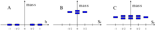
Figure 1: The mass spectrum.

3.3 Nondecoupling of $U(1)$ from $SU(N)$ and NGF-related vertices

In this section, we will see that the overall $U(1)$ gauge part (in which the NGF resides) does not decouple from the other part in the lagrangian. To see this we concentrate on the Yukawa interaction terms.

As in appendix A, the Yukawa couplings are contained in ${\mathcal{L}}_{\rm{mass}}$ (A.17) and ${\mathcal{L}}_{\rm{kin}}$ (A). Let us write them down for convenience:

$${\mathcal{L}}_{\rm{mass}} = -\frac{\sqrt{2N}}{2}m{\mathcal{F}}_{0ab}\psi^{a}\psi^{b}-\frac{i\sqrt{2N}}{4}g^{ab}(e\delta^{0}_{a}+m{\mathcal{F}}_{0a}){\mathcal{F}}_{bcd}\psi^{c}\psi^{d}$$

$$-\frac{i\sqrt{2N}}{4}g^{ab}(\bar{e}\delta^{0}_{a}+m\bar{{\mathcal{F}}}_{0a}){\mathcal{F}}_{bcd}\lambda^{c}\lambda^{d}+\frac{1}{\sqrt{2}}g_{ab}f^{b}_{cd}\bar{\phi}^{d}\lambda^{c}\psi^{a}-\frac{1}{4\sqrt{2}}f^{a}_{bc}\bar{\phi}^{b}\phi^{c}{\mathcal{F}}_{ade}\psi^{d}\lambda^{e}+c.c.,$$

$${\mathcal{L}}_{\rm{kin}} = -\frac{1}{2}{\mathcal{F}}_{ab}\lambda^{a}\sigma^{\mu}\mathcal{D}_{\mu}\bar{\lambda}^{b}-\frac{i}{2}g_{ab}\psi^{a}\sigma^{\mu}\mathcal{D}_{\mu}\bar{\psi}^{b}+c.c.+\ldots,$$ (3.36)

where we have substituted the explicit form of the superpotential (3.30) into (A.17).

Let us consider the model on the vacua with partially and spontaneously broken supersymmetry. We expand the scalar fields around the vacuum expectation values as

$$\phi^{a}=\langle\phi^{a}\rangle+\tilde{\phi}^{a}.$$ (3.37)

We expand the prepotential and other quantities, e.g., $\mathcal{F}_{abc}=\langle\mathcal{F}_{abc}\rangle+\langle\mathcal{F}_{abcd}\rangle\tilde{\phi}^{d}+\dots$ in the fluctuation field $\tilde{\phi}$,

Let us list the Yukawa couplings obtained from ${\mathcal{L}}_{{\rm mass}}$ (3.3). From the first and second terms, the $\psi\psi\phi$ vertices are

$$\frac{\sqrt{2N}}{4}m\langle-2i{\mathcal{F}}_{0abc}+g^{de}{\mathcal{F}}_{abe}{\mathcal{F}}_{0cd}\rangle\tilde{\phi}^{c}\psi^{a}\psi^{b}.$$ (3.38)

Note that we have included $i$ factor in front of the interaction lagrangian. The $\lambda\lambda\bar{\phi}$ vertices are calculated from the third term of (3.3):

$$\frac{\sqrt{2N}}{4}m\langle g^{de}{\mathcal{F}}_{abe}\bar{{\mathcal{F}}}_{0cd}\rangle\bar{\tilde{\phi}}^{c}\lambda^{a}\lambda^{b}.$$ (3.39)

From the last two terms, we obtain the $\lambda\psi\phi$ ($\lambda\psi\bar{\phi}$) vertices

$$\frac{1}{4\sqrt{2}}\langle 2f^{b}_{cd}{\mathcal{F}}_{abe}\bar{\phi}^{d}-f^{b}_{de}{\mathcal{F}}_{abc}\bar{\phi}^{d}\rangle\tilde{\phi}^{e}\lambda^{c}\psi^{a}$$

$$+\frac{1}{4\sqrt{2}}\langle 4if^{b}_{ce}g_{ab}-2f^{b}_{cd}\bar{{\mathcal{F}}}_{abe}\bar{\phi}^{d}-f^{b}_{ed}{\mathcal{F}}_{abc}\phi^{d}\rangle\bar{\tilde{\phi}}^{e}\lambda^{c}\psi^{a}.$$ (3.40)

There are also derivative coupling terms obtained from ${\mathcal{L}}_{{\rm kin}}$ (3.36). The Feynman rules are illustrated in Fig. 2 and 3. The propagator of the massless $\lambda$ fermions and that of massive $\psi$ fermions are denoted by a single line and a double solid line respectively. The scalar propagator is drawn by a broken line.

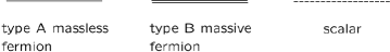
Figure 2: Feynman propagators for the massless and massive fermions and the scalar. That of type A massless fermions, i.e., $\lambda^{a}$ is drawn by a single solid line while that of type B massive fermions, i.e., $\psi^{a}$ is drawn by a double solid lines. A scalar propagator is drawn by a broken line.

Figure 3: A Feynman rule for three-point vertices corresponding to (3.38), (3.39) and (3.40).

Next, we focus on the Yukawa coupling involving one NGF. Such couplings can be obtained from $\lambda\lambda\phi$ and $\psi\lambda\phi$ vertices in ${\mathcal{L}}_{{\rm mass}}$. From (3.39), it can be easily seen that the coupling of the NGF and the $SU(N)$ fermions are indeed nonvanishing:

$$\frac{\sqrt{2N}}{4}m\langle g^{de}{\mathcal{F}}_{0be}\bar{{\mathcal{F}}}_{0cd}\rangle\bar{\tilde{\phi}}^{c}\lambda^{0}\lambda^{b}=\frac{\sqrt{2N}}{4}m\sum_{\alpha}\langle g^{\alpha\alpha}|{\mathcal{F}}_{0\alpha\alpha}|^{2}\rangle\tilde{\phi}^{\alpha}\lambda^{0}\lambda^{\alpha}.$$ (3.41)

Note that we have used $\langle{\mathcal{F}}_{0\mu\nu}\rangle=0$ [10], where $\mu$ label the broken non-Cartan generators. Eq. (3.41) means that the Yukawa coupling of the NGF with the fermions belonging to the unbroken generators does exist. The existence of the nonderivative Yukawa coupling that involves the NGF and that is supported by the third prepotential derivatives is remarkable.

The coupling coming from (3.40) vanishes because $f^{0}_{ab}=0$ and $f^{r}_{ab}\langle\phi^{a}\rangle=0$ which follows from $[t_{r},\langle\phi\rangle]=0$. There are also derivative couplings due to ${\mathcal{L}}_{{\rm kin}}$.

4 Low energy suppression of NGF emission by direct computation

In this section, we check the validity of the low energy theorem stated in section 2 by direct computation of tree Feynman diagrams obtained from the lagrangian. According to our discussion of the $U(1)$ nondecoupling and the presence of nonderivative couplings of the NGF and the $SU(N)$ sector, the low energy suppression of processes having the emission of the NGF together with massless as well as massive particles in the final state is by no means obvious. We will exhibit a cancellation mechanism shortly.

For simplicity and illustrative purposes, we take as an initial state two massive fermions of type B with momentum $p^{a}$ and $p^{b}$. In the final state, we consider the case in which the NGF with momentum $p^{0}$ and massless fermion (gaugino) of type A with momentum $p^{\alpha}$ are present. We limit ourselves to this case, namely, $\psi^{a}\psi^{b}\rightarrow\lambda^{0}\lambda^{\alpha}$ scattering in this paper, as in Fig.4.

The nonvanishing possibilities are $(a,b)=(\alpha,0)$. As for the diagram of $t$-channel scalar exchange, the relevant interaction vertex can in principle be obtained from (3.40). But, as explained in subsection 3.3, it vanishes for the NGF as the piece of the structure constant is zero in which overall $U(1)$ is involved.

In order to discuss the diagram of $s$-channel annihilation, it is more transparent to extract the appropriate effective $(\psi\psi)(\lambda\lambda)$ vertex with one scalar contraction from $\frac{1}{2}\left(i\int{\mathcal{L}}_{{\rm mass}}\right)^{2}$. Rescaling the fluctuation field as $\tilde{\phi}^{a}=\sqrt{g^{aa}}\phi^{a}_{can}$, we obtain

$$\frac{1}{16}(\sqrt{2N}m)^{2}\langle g^{ab}\bar{{\mathcal{F}}}_{0be}\sqrt{g^{ee}}{\mathcal{F}}_{acd}\rangle\langle g^{hi}{\mathcal{F}}_{0hf}\sqrt{g^{ff}}{\mathcal{F}}_{ijk}-2i{\mathcal{F}}_{0hif}\sqrt{g^{ff}}\rangle$$ (4.1)

$$~{}~{}~{}~{}~{}~{}\times\int d^{4}x_{1}d^{4}x_{2}\langle\phi^{*e}_{can}(x_{1})\phi^{f}_{can}(x_{2})\rangle(\lambda^{c}\lambda^{d})(x_{1})(\psi^{j}\psi^{k})(x_{2})\;.$$

Note that

$${\rm F.T.}\left(\langle\phi^{*e}_{can}(x_{1})\phi^{f}_{can}(x_{2})\rangle\right)(p_{0},p_{\alpha})=\frac{-i\delta_{ef}}{m_{\alpha}^{2}-(p_{0}+p_{\alpha})^{2}}$$ (4.2)

as well as

$$m_{\alpha}^{2}=2Nm^{2}\langle g^{\alpha\alpha}\rangle^{2}\langle{\mathcal{F}}_{0\alpha\alpha}\rangle\langle\bar{{\mathcal{F}}}_{0\alpha\alpha}\rangle\;.$$ (4.3)

In the limit of $p_{0}\rightarrow 0$, the propagator is $\frac{-i}{m_{\alpha}^{2}}$, and the contribution to the $\psi^{a}\psi^{b}\rightarrow\lambda^{0}\lambda^{\alpha}$ scattering amplitude from eq. (4.1) is

$$-\frac{1}{8}\langle{\mathcal{F}}_{00\alpha\alpha}\rangle-\frac{i}{16}\langle g^{\alpha\alpha}\rangle\langle{\mathcal{F}}_{0\alpha\alpha}\rangle^{2}\;.$$ (4.4)

The presence of this alone is against the low energy theorem and is in fact saved by the presence of the appropriate four-Fermi interactions in (A.18). Their contributions are

$$\frac{1}{8}\langle{\mathcal{F}}_{00\alpha\alpha}\rangle+\frac{i}{16}\langle g^{\alpha\alpha}\rangle(\langle{\mathcal{F}}_{0\alpha\alpha}\rangle)^{2}\;,$$ (4.5)

exactly cancelling eq. (4.4).

Figure 4: $\psi^{0}\psi^{\alpha}\rightarrow\lambda^{0}\lambda^{\alpha}$ tree diagrams.

Appendix

Appendix A The component Lagrangian

In this appendix, we consider the lagrangian of ${\mathcal{N}}=2$ supersymmetric $U(N)$ gauge theory with the electric and magnetic FI terms in terms of the component fields. We use convention of [39]. In particular, we use the metric $\eta^{\mu\nu}=\mathrm{diag}(+1,-1,-1,-1)$ and the Levi-Civita symbol $\epsilon_{0123}=+1$ and $\epsilon^{0123}=-1$.

The lagrangian (3.1) can be divided into the following parts:

$${\mathcal{L}}={\mathcal{L}}_{{\rm Kahler}}+{\mathcal{L}}_{{\rm gauge}}+\left[\int d^{2}\theta W+c.c.\right],$$ (A.1)

where

$${\mathcal{L}}_{{\rm Kahler}} = \mathop{\rm Im}\left[\int d^{4}\theta{\rm Tr}\bar{\Phi}e^{adV}\frac{\partial{\mathcal{F}}(\Phi)}{\partial\Phi}\right],$$

$${\mathcal{L}}_{{\rm gauge}} = \mathop{\rm Im}\left[\int d^{2}\theta\frac{1}{2}{\mathcal{F}}_{ab}{\mathcal{W}}^{\alpha a}{\mathcal{W}}^{b}_{\alpha}\right],$$ (A.2)

We have chosen the common function ${\mathcal{F}}$ in Kähler, gauge kinetic and superpotential terms such that the lagrangian is invariant under the discrete R transformation (3.7).

In components, as can be seen in appendix of [14], ${\mathcal{L}}_{{\rm Kahler}}$ is the same as ${\mathcal{L}}_{K}+{\mathcal{L}}_{\Gamma}$ in the original lagrangian of [9], which is

$${\mathcal{L}}_{{\rm Kahler}} = g_{ab}{\mathcal{D}}_{\mu}\phi^{a}{\mathcal{D}}^{\mu}\bar{\phi}^{b}-\frac{i}{2}g_{ab}\psi^{a}\sigma^{\mu}{\mathcal{D}}_{\mu}^{\prime}\bar{\psi}^{b}+\frac{i}{2}g_{ab}{\mathcal{D}}_{\mu}^{\prime}\psi^{a}\sigma^{\mu}\bar{\psi}^{b}+g_{ab}F^{a}\bar{F}^{b}$$ (A.3)

$$-\frac{1}{2}g_{ab,\bar{c}}F^{a}\bar{\psi}^{b}\bar{\psi}^{c}-\frac{1}{2}g_{bc,a}\bar{F}^{c}\psi^{a}\psi^{b}+\frac{1}{\sqrt{2}}g_{ab}(\lambda^{c}\psi^{a}k_{c}^{*}{}^{b}+\bar{\lambda}^{c}\bar{\psi}^{b}k_{c}{}^{a})+\frac{1}{2}D^{a}\mathfrak{D}_{a}~{},$$

where $g_{ab}$ is the Kähler metric and its derivatives are defined as $g_{ab,c}\equiv\partial g_{ab}/\partial\phi^{c}$ and $g_{ab,\bar{c}}\equiv\partial g_{ab}/\partial\bar{\phi}^{c}$. The covariant derivatives are defined as

$${\mathcal{D}}_{\mu}\phi^{a} = \partial_{\mu}\phi^{a}-\frac{1}{2}A_{\mu}^{b}k_{b}{}^{a},$$ (A.4)

$${\mathcal{D}}_{\mu}^{\prime}\psi^{a} = {\mathcal{D}}_{\mu}\psi^{a}+\Gamma^{a}_{bc}({\mathcal{D}}_{\mu}\phi^{b})\psi^{c},$$ (A.5)

$${\mathcal{D}}_{\mu}\psi^{a} = \partial_{\mu}\psi^{a}-\frac{1}{2}A_{\mu}^{b}\partial_{c}k_{b}{}^{a}\psi^{c}~{},$$ (A.6)

where $\Gamma^{a}_{bc}=g^{ad}g_{bd,c}$. Also, the Killing vector and the Killing potential are given by

$$k_{a} = k_{a}^{b}\partial_{b},~{}~{}~{}k_{a}^{b}=-ig^{bc}\bar{\partial}_{c}\mathfrak{D}_{a},$$

$$\mathfrak{D}_{a} = -\frac{1}{2}({\mathcal{F}}_{b}f^{b}_{ac}\bar{\phi}^{c}+\bar{{\mathcal{F}}}_{b}f^{b}_{ac}\phi^{c}),$$ (A.7)

which satisfies [9]

$$k_{b}^{c}\partial_{c}\Phi^{a}=f^{a}_{bc}\Phi^{c},~{}~{}~{}k_{b}^{c}\partial_{c}{\mathcal{F}}_{a}=-f^{a}_{bc}{\mathcal{F}}_{a}.$$ (A.8)

By using the second equation of (A.8): ${\mathcal{F}}_{b}f_{ac}^{b}=k_{c}^{d}\partial_{d}{\mathcal{F}}_{a}={\mathcal{F}}_{ad}f^{d}_{ce}\phi^{e}$, the Killing potential (A.7) can be written as

$$\mathfrak{D}_{a}=-\frac{1}{2}f^{b}_{cd}\bar{\phi}^{c}\phi^{d}({\mathcal{F}}_{ab}-\bar{{\mathcal{F}}}_{ab})=-ig_{ab}f^{b}_{cd}\bar{\phi}^{c}\phi^{d}.$$ (A.9)

The gauge part ${\mathcal{L}}_{{\rm gauge}}$ is, in components,

$${\mathcal{L}}_{{\rm gauge}} = -\frac{1}{2}{\mathcal{F}}_{ab}\lambda^{a}\sigma^{\mu}{\mathcal{D}}_{\mu}\bar{\lambda}^{b}-\frac{1}{2}\bar{{\mathcal{F}}}_{ab}{\mathcal{D}}_{\mu}\lambda^{a}\sigma^{\mu}\bar{\lambda}^{b}-\frac{1}{4}g_{ab}F_{\mu\nu}^{a}F^{b\mu\nu}-\frac{1}{8}({\mathrm{Re}}{\mathcal{F}})_{ab}\epsilon^{\mu\nu\rho\sigma}F_{\mu\nu}^{a}F_{\rho\sigma}^{b}$$ (A.10)

$$-\frac{\sqrt{2}i}{8}({\mathcal{F}}_{abc}\psi^{c}\sigma^{\nu}\bar{\sigma}^{\mu}\lambda^{a}-\bar{{\mathcal{F}}}_{abc}\bar{\lambda}^{a}\bar{\sigma}^{\mu}\sigma^{\nu}\bar{\psi}^{c})F_{\mu\nu}^{b}$$

$$+\frac{1}{2}g_{ab}D^{a}D^{b}+\frac{\sqrt{2}}{4}({\mathcal{F}}_{abc}\psi^{c}\lambda^{a}+\bar{{\mathcal{F}}}_{abc}\bar{\psi}^{c}\bar{\lambda}^{a})D^{b}+\frac{i}{4}{\mathcal{F}}_{abc}F^{c}\lambda^{a}\lambda^{b}-\frac{i}{4}\bar{{\mathcal{F}}}_{abc}\bar{F}^{c}\bar{\lambda}^{a}\bar{\lambda}^{b}$$

$$-\frac{i}{8}{\mathcal{F}}_{abcd}\psi^{c}\psi^{d}\lambda^{a}\lambda^{b}+\frac{i}{8}\bar{{\mathcal{F}}}_{abcd}\bar{\psi}^{c}\bar{\psi}^{d}\bar{\lambda}^{a}\bar{\lambda}^{b},$$

where the field strength is $F_{\mu\nu}^{a}=\partial_{\mu}A_{\nu}^{a}-\partial_{\nu}A_{\mu}^{a}-\frac{1}{2}f^{a}_{bc}A_{\mu}^{b}A_{\nu}^{c}$. Finally, the superpotential can be written as

$$\int d^{2}\theta W(\Phi)+c.c. = F^{a}\partial_{a}W-\frac{1}{2}\partial_{a}\partial_{b}W\psi^{a}\psi^{b}+c.c..$$ (A.11)

Let us exhibit the on-shell Lagrangian. Eq. of motion with respect to the auxiliary fields $D^{a}$ and $F^{a}$ are

$$D^{a} = -\frac{1}{2}g^{ab}\mathfrak{D}_{b}-\frac{1}{2\sqrt{2}}g^{ab}\left({\mathcal{F}}_{bcd}\psi^{d}\lambda^{c}+\bar{{\mathcal{F}}}_{bcd}\bar{\psi}^{d}\bar{\lambda}^{c}\right),$$

$$F^{a} = -g^{ab}\overline{\partial_{b}W}-\frac{i}{4}g^{ab}\left({\mathcal{F}}_{bcd}\psi^{c}\psi^{d}-\bar{{\mathcal{F}}}_{bcd}\bar{\lambda}^{c}\bar{\lambda}^{d}\right),$$ (A.12)

where $g^{ab}$ are defined by $g_{ab}g^{bc}=\delta^{c}_{a}$. After eliminating the auxiliary fields, the lagrangian ${\mathcal{L}}$ reduces to the following on-shell Lagrangian:

$${\mathcal{L}}_{{\rm on-shell}} = {\mathcal{L}}_{\rm{kin}}+{\mathcal{L}}_{\rm{pot}}+{\mathcal{L}}_{\rm{Pauli}}+{\mathcal{L}}_{\rm{mass}}+{\mathcal{L}}_{\rm{fermi^{4}}},$$ (A.13)

where

$${\mathcal{L}}_{\rm{kin}} = g_{ab}\mathcal{D}_{\mu}\phi^{a}\mathcal{D}^{\mu}\bar{\phi}^{b}-\frac{1}{4}g_{ab}F_{\mu\nu}^{a}F^{b\mu\nu}-\frac{1}{8}({\mathrm{Re}}{\mathcal{F}})_{ab}\epsilon^{\mu\nu\rho\sigma}F_{\mu\nu}^{a}F_{\rho\sigma}^{b}$$

$$-\frac{1}{2}{\mathcal{F}}_{ab}\lambda^{a}\sigma^{\mu}\mathcal{D}_{\mu}\bar{\lambda}^{b}-\frac{1}{2}\bar{{\mathcal{F}}}_{ab}\mathcal{D}_{\mu}\lambda^{a}\sigma^{\mu}\bar{\lambda}^{b}-\frac{i}{2}g_{ab}\psi^{a}\sigma^{\mu}\mathcal{D}_{\mu}\bar{\psi}^{b}+\frac{i}{2}g_{ab}\mathcal{D}_{\mu}\psi^{a}\sigma^{\mu}\bar{\psi}^{b},$$

$${\mathcal{L}}_{\rm{pot}} = -\frac{1}{8}g^{ab}\mathfrak{D}_{a}\mathfrak{D}_{b}-g^{ab}\partial_{a}W\overline{\partial_{b}W}=-V,$$ (A.15)

$${\mathcal{L}}_{\rm{Pauli}} = -\frac{i}{4\sqrt{2}}{\mathcal{F}}_{abc}\psi^{c}\sigma^{\nu}\bar{\sigma}^{\mu}\lambda^{a}F_{\mu\nu}^{b}+\frac{i}{4\sqrt{2}}\bar{{\mathcal{F}}}_{abc}\bar{\lambda}^{a}\bar{\sigma}^{\mu}\sigma^{\nu}\bar{\psi}^{c}F_{\mu\nu}^{b},$$ (A.16)

$${\mathcal{L}}_{\rm{mass}} = -\frac{1}{2}\partial_{a}\partial_{b}W\psi^{a}\psi^{b}-\frac{i}{4}g^{ab}\partial_{a}W\left({\mathcal{F}}_{bcd}\psi^{c}\psi^{d}-\bar{{\mathcal{F}}}_{bcd}\bar{\lambda}^{c}\bar{\lambda}^{d}\right)$$ (A.17)

$$-\frac{1}{2}\overline{\partial_{a}\partial_{b}W}\bar{\psi}^{a}\bar{\psi}^{b}-\frac{i}{4}g^{ab}\overline{\partial_{a}W}\left({\mathcal{F}}_{bcd}\lambda^{c}\lambda^{d}-\bar{{\mathcal{F}}}_{bcd}\bar{\psi}^{c}\bar{\psi}^{d}\right)$$

$$+\frac{1}{\sqrt{2}}g_{ab}\left(\bar{\lambda^{c}}\bar{\psi}^{b}k_{c}{}^{a}+\lambda^{c}\psi^{a}k_{c}^{*}{}^{b}\right)-\frac{1}{4\sqrt{2}}g^{ab}\mathfrak{D}_{a}\left({\mathcal{F}}_{bcd}\psi^{d}\lambda^{c}+\bar{{\mathcal{F}}}_{bcd}\bar{\psi}^{d}\bar{\lambda}^{c}\right),$$

$${\mathcal{L}}_{\rm{fermi^{4}}} = -\frac{i}{8}{\mathcal{F}}_{abcd}\psi^{a}\psi^{b}\lambda^{c}\lambda^{d}+\frac{i}{8}\bar{{\mathcal{F}}}_{abcd}\bar{\psi}^{a}\bar{\psi}^{b}\bar{\lambda}^{c}\bar{\lambda}^{d}$$ (A.18)

$$-\frac{1}{16}g^{ab}\left({\mathcal{F}}_{acd}\psi^{d}\lambda^{c}+\bar{{\mathcal{F}}}_{acd}\bar{\psi}^{d}\bar{\lambda}^{c}\right)\left({\mathcal{F}}_{bef}\psi^{f}\lambda^{e}+\bar{{\mathcal{F}}}_{bef}\bar{\psi}^{f}\bar{\lambda}^{e}\right)$$

$$+\frac{1}{16}g^{ab}\left({\mathcal{F}}_{acd}\lambda^{c}\lambda^{d}-\bar{{\mathcal{F}}}_{acd}\bar{\psi}^{c}\bar{\psi}^{d}\right)\left({\mathcal{F}}_{bef}\psi^{e}\psi^{f}-\bar{{\mathcal{F}}}_{bef}\bar{\lambda}^{e}\bar{\lambda}^{f}\right).$$

In (A.15), we have used that $\mathfrak{D}_{a}g^{ab}\delta_{b}^{0}=-if^{0}_{ab}\bar{\phi}^{a}\phi^{b}=0$, following from (A.9).

Appendix B Supersymmetry transformation law

We consider supersymmetry transformation laws in this subsection. The first and second ${\mathcal{N}}=1$ supersymmetry transformation laws of the scalar and the fermions are (see [39]):

$$\delta_{\eta_{1}}\phi^{a} = \sqrt{2}\eta_{1}\psi^{a},$$

$$\delta_{\eta_{1}}\psi^{a} = i\sqrt{2}\sigma^{\mu}\bar{\eta}_{1}{\mathcal{D}}_{\mu}\phi^{a}+\sqrt{2}\eta_{1}F^{a},$$

$$\delta_{\eta_{1}}\lambda^{a} = \sigma^{\mu\nu}\eta_{1}F_{\mu\nu}^{a}+i\eta_{1}D^{a},$$

$$\delta_{\eta_{1}}A_{\mu}^{a} = -i\eta_{1}\sigma_{\mu}\bar{\lambda}^{a}+i\lambda^{a}\sigma_{\mu}\bar{\eta}_{1},$$ (B.1)

and

$$\delta_{\eta_{2}}\phi^{a} = -\sqrt{2}\eta_{2}\lambda^{a},$$

$$\delta_{\eta_{2}}\lambda^{a} = -i\sqrt{2}\sigma^{\mu}\bar{\eta}_{2}{\mathcal{D}}_{\mu}\phi^{a}-\sqrt{2}\eta_{2}\widetilde{F}^{a},$$

$$\delta_{\eta_{2}}\psi^{a} = \sigma^{\mu\nu}\eta_{2}F_{\mu\nu}^{a}+i\eta_{2}\widetilde{D}^{a},$$

$$\delta_{\eta_{2}}A_{\mu}^{a} = -i\eta_{2}\sigma_{\mu}\bar{\psi}^{a}+i\psi^{a}\sigma_{\mu}\bar{\eta}_{2},$$ (B.2)

where $\eta_{1}$ and $\eta_{2}$ are the transformation parameters of the first ${\mathcal{N}}=1$ supersymmetry and the second one respectively. The second supersymmetry transformation is derived by acting the discrete R transformation on the first one, as explained in section 3. Also, the auxiliary fields are defined in (A.12) and

$$\widetilde{D}^{a} = -\frac{1}{2}g^{ab}\mathfrak{D}_{b}+\frac{1}{2\sqrt{2}}g^{ab}\left({\mathcal{F}}_{bcd}\psi^{d}\lambda^{c}+\bar{{\mathcal{F}}}_{bcd}\bar{\psi}^{d}\bar{\lambda}^{c}\right),$$

$$\widetilde{F}^{a} = -\sqrt{2N}g^{ab}(e\delta_{b}^{0}+m\bar{{\mathcal{F}}}_{0b})-\frac{i}{4}g^{ab}\left({\mathcal{F}}_{bcd}\lambda^{c}\lambda^{d}-\bar{{\mathcal{F}}}_{bcd}\bar{\psi}^{c}\bar{\psi}^{d}\right).$$ (B.3)

We note that the sign of $\mathop{\rm Im}e$ has been flipped in $\widetilde{F}$ as compared with $F$ in (A.12).

These supersymmetry transformation laws (B.1) and (B.2) can be combined into the following forms:

$$\delta\phi^{a} = \sqrt{2}\left(\begin{array}[]{cc}\psi^{a}&-\lambda^{a}\end{array}\right)\left(\begin{array}[]{c}\eta_{1}\\ \eta_{2}\end{array}\right),$$ (B.7)

$$\delta\left(\begin{array}[]{c}\lambda^{a}\\ \psi^{a}\end{array}\right) = F_{\mu\nu}^{a}\sigma^{\mu\nu}\left(\begin{array}[]{c}\eta_{1}\\ \eta_{2}\end{array}\right)-i\sqrt{2}\sigma^{\mu}\left(\begin{array}[]{c}\bar{\eta}_{2}\\ -\bar{\eta}_{1}\end{array}\right){\mathcal{D}}_{\mu}\phi^{a}+\left(\begin{array}[]{cc}iD^{a}&-\sqrt{2}\widetilde{F}^{a}\\ \sqrt{2}F^{a}&i\widetilde{D}^{a}\end{array}\right)\left(\begin{array}[]{c}\eta_{1}\\ \eta_{2}\end{array}\right),$$ (B.18)

$$\delta A_{\mu}^{a} = i\left(\begin{array}[]{cc}\bar{\lambda}^{a}&\bar{\psi}^{a}\end{array}\right)\bar{\sigma}_{\mu}\left(\begin{array}[]{c}\eta_{1}\\ \eta_{2}\end{array}\right)+i\left(\begin{array}[]{cc}\psi^{a}&-\lambda^{a}\end{array}\right)\sigma_{\mu}\left(\begin{array}[]{c}\bar{\eta}_{2}\\ -\bar{\eta}_{1}\end{array}\right)$$ (B.25)

where $\delta\Psi\equiv\delta_{\eta_{1}}\Psi+\delta_{\eta_{2}}\Psi$. The last term of the transformation law of the fermion doublet can be separated into the terms involving the fermion bilinears and the other terms. This last part is

$$-\frac{i}{2}g^{ab}\mathfrak{D}_{b}\left(\begin{array}[]{c}\eta_{1}\\ \eta_{2}\end{array}\right)+2\sqrt{N}g^{ab}\left(\begin{array}[]{cc}-i\xi&(e\delta_{b}^{0}+m\bar{{\mathcal{F}}}_{0b})\\ -(\bar{e}\delta_{b}^{0}+m\bar{{\mathcal{F}}}_{0b})&i\xi\end{array}\right)\left(\begin{array}[]{c}\eta_{1}\\ \eta_{2}\end{array}\right).$$ (B.32)

Appendix C ${\mathcal{N}}=1$ supercurrent and the low energy theorem

In this appendix, we briefly review the low energy theorem for the scattering amplitudes in the case where ${\mathcal{N}}=1$ supersymmetry is spontaneously and completely broken [4]. We consider the special case where supersymmetry is broken by the Fayet-Iliopoulos D-term [40]. The supercurrent in the four component majorana notation reads

$${\mathcal{S}}^{\mu}=-if_{\lambda}\gamma^{\mu}\lambda+\frac{1}{2}F_{\nu\rho}\gamma^{\nu}\gamma^{\rho}\gamma^{\mu}\gamma_{5}\lambda+\ldots$$ (C.1)

where $\lambda$ is the NGF field and $f_{\lambda}$ is the decay constant. $F_{\mu\nu}$ is a field strength of an abelian gauge field.

Let us look at the following scattering processes: (1) processes of the type $A\rightarrow B+\lambda$; (2) radiative processes of the type $A\rightarrow B+\gamma+\lambda$. We denote the corresponding amplitudes by $\bar{u}(q)M_{1}(q)$ and $\epsilon^{*}_{\mu}(k)\bar{u}(q)M_{2}^{\mu}(k,q)$ respectively. $A$ and $B$ are respectively the initial and the final multiparticle states consisting of massive particles alone.

(1) First, consider the matrix element of the form

$$\langle B|{\mathcal{S}}^{\mu}|A\rangle.$$ (C.2)

In the diagrammatic representation, the possible insertions of the supercurrent ${\mathcal{S}}^{\mu}$ are divided into three patterns as depicted in Fig. 5. In the limit $q^{\mu}\rightarrow 0$, the contributions to the amplitude from Fig. 5-1 and from Fig. 5-2 can be singular and that from Fig. 5-3 is regular. In fact, the contribution from Fig. 5-1, in terms of the amplitude $M_{1}$ above, reads

$$\langle 0|{\mathcal{S}}^{\mu}|\lambda\rangle\times\frac{iq^{\mu}\gamma_{\mu}}{q^{2}}\times M_{1}(q)\;,$$ (C.3)

which is singular as $q^{\mu}\rightarrow 0$. Fig. 5-2 can be singular in the limit as well for the case in which masses of the two particles coupling to the current are degenerate. This is seen as follows: suppose that we insert ${\mathcal{S}}^{\mu}$ in an initial external line whose momentum and mass are $p_{i}$ and $m_{i}$ respectively. The propagator that connects to this line via the current insertion is, for the case of a scalar,

$$\frac{i}{(p_{i}+q)^{2}-m_{j}^{2}}=\frac{i}{m_{i}^{2}-m_{j}^{2}+2p_{i}\cdot q+{\mathcal{O}}(q^{2})},$$ (C.4)

where $m_{j}$ is the mass of the intermediate state that propagates. A similar expression holds for a fermion. Thus, only when the masses are degenerate, $m_{i}=m_{j}$, (C.4) is singular as $q^{\mu}\rightarrow 0$. Under the assumption that there is no such degeneracy, Fig. 5-2 does not contribute. The conservation of the current $\partial_{\mu}\langle B|{\mathcal{S}}^{\mu}|A\rangle=0$ leads to

$$\lim_{q^{\mu}\rightarrow 0}M_{1}=0.$$ (C.5)

The processes of this type with the NGF emission are suppressed.

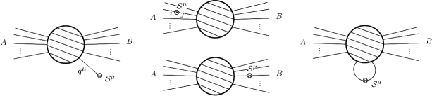
Figure 5: Insertions of ${\mathcal{S}}^{\mu}$ which are denoted by a crossed circle. Fig. 5-1) ${\mathcal{S}}^{\mu}$ is inserted in the end point of the NGF propagator (one-point coupling). Fig. 5-2) ${\mathcal{S}}^{\mu}$ is inserted in an initial or a final external line (two-point coupling). Fig. 5-3) ${\mathcal{S}}^{\mu}$ is connected to internal lines.

(2) Next, consider the processes of the second type with both photon emission and NGF emission. The diagrams with current insertion that give rise to singular contributions are illustrated in Fig. 6. Contrary to the processes considered in (1), Fig. 6-2 gives a nonvanishing contribution as both photon and the NGF are massless. The supercurrent (C.1) in fact contains a $\gamma$-$\lambda$ coupling, which is the second term in (C.1). Note that we can relate the radiative amplitude of this type with the amplitude $M_{1}$ discussed in (1) by the current conservation. In fact, $\partial_{\mu}\langle B,\gamma|{\mathcal{S}}^{\mu}|A\rangle$, leads to

$$\lim_{q\rightarrow 0}\epsilon^{*}_{\mu}M_{2}^{\mu}(q,k)=-if^{-1}_{\lambda}\epsilon^{*}_{\mu}k_{\nu}\gamma^{\mu}\gamma^{\nu}\gamma_{5}M_{1}(k).$$ (C.6)

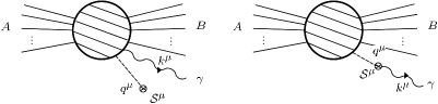
Figure 6: Fig. 6-1) ${\mathcal{S}}^{\mu}$ is inserted in the end point of the NGF propagator (one-point coupling.) Fig. 6-2) ${\mathcal{S}}^{\mu}$ is inserted in the external photon line (two-point coupling.)

References

• [1] Y. Nambu, Phys. Rev. Lett.  4 (1960) 380.
• [2] Y. Nambu and G. Jona-Lasinio, Phys. Rev.  122 (1961) 345; Phys. Rev.  124 (1961) 246.
• [3] See, for instance, S. L. Adler and R. F. Dashen, “Current Algebras and Applications to Particle Physics,” Benjamin, New York (1968) 394p; M. Bando, T. Kugo and K. Yamawaki, Phys. Rept.  164 (1988) 217; T. Kugo, “Quantum Theory of Gauge Field,” volume I and II, chapter 6, Baifukan (1989) 272p and 284p.
• [4] B. de Wit and D. Z. Freedman, Phys. Rev. Lett.  35 (1975) 827.
• [5] B. de Wit and D. Z. Freedman, Phys. Rev.  D 12 (1975) 2286.
• [6] W. A. Bardeen, (1975) unpublished; W. A. Bardeen and V. Visnjic, Nucl. Phys.  B 194 (1982) 422.
• [7] R. Kallosh and T. Kugo, JHEP 0901 (2009) 072 [arXiv:0811.3414 [hep-th]].
• [8] I. Antoniadis, H. Partouche and T. R. Taylor, Phys. Lett.  B 372, 83 (1996) [arXiv:hep-th/9512006]; S. Ferrara, L. Girardello and M. Porrati, Phys. Lett.  B 376 (1996) 275 [arXiv:hep-th/9512180]; E. A. Ivanov and B. M. Zupnik, Phys. Atom. Nucl.  62, 1043 (1999) [Yad. Fiz.  62, 1110 (1999)] [arXiv:hep-th/9710236]; T. R. Taylor and C. Vafa, Phys. Lett.  B 474 (2000) 130 [arXiv:hep-th/9912152].
• [9] K. Fujiwara, H. Itoyama and M. Sakaguchi, Prog. Theor. Phys.  113 (2005) 429 [arXiv:hep-th/0409060]; arXiv:hep-th/0410132.
• [10] K. Fujiwara, H. Itoyama and M. Sakaguchi, Nucl. Phys.  B 723 (2005) 33 [arXiv:hep-th/0503113]; Prog. Theor. Phys. Suppl.  164 (2007) 125 [arXiv:hep-th/0602267].
• [11] K. Fujiwara, H. Itoyama and M. Sakaguchi, Nucl. Phys.  B 740 (2006) 58 [arXiv:hep-th/0510255]; AIP Conf. Proc.  903 (2007) 521 [arXiv:hep-th/0611284].
• [12] P. Kaste and H. Partouche, JHEP 0411 (2004) 033 [arXiv:hep-th/0409303]; P. Merlatti, Nucl. Phys.  B 744 (2006) 207 [arXiv:hep-th/0511280]; I. Antoniadis, J. P. Derendinger and T. Maillard, Nucl. Phys.  B 808 (2009) 53 [arXiv:0804.1738 [hep-th]].
• [13] H. Itoyama and K. Maruyoshi, Phys. Lett.  B 650 (2007) 298 [arXiv:0704.1060 [hep-th]]; K. Maruyoshi, arXiv:0710.2154 [hep-th].
• [14] H. Itoyama and K. Maruyoshi, Nucl. Phys.  B 796 (2008) 246 [arXiv:0710.4377 [hep-th]].
• [15] K. Fujiwara, Nucl. Phys.  B 770 (2007) 145 [arXiv:hep-th/0609039].
• [16] N. Seiberg and E. Witten, Nucl. Phys.  B 426 (1994) 19 [Erratum-ibid.  B 430 (1994) 485] [arXiv:hep-th/9407087]; Nucl. Phys.  B 431 (1994) 484 [arXiv:hep-th/9408099].
• [17] C. Vafa, J. Math. Phys.  42 (2001) 2798 [arXiv:hep-th/0008142].
• [18] F. Cachazo, K. A. Intriligator and C. Vafa, Nucl. Phys.  B 603 (2001) 3 [arXiv:hep-th/0103067].
• [19] R. Dijkgraaf and C. Vafa, Nucl. Phys.  B 644 (2002) 3 [arXiv:hep-th/0206255]; Nucl. Phys.  B 644 (2002) 21 [arXiv:hep-th/0207106]; arXiv:hep-th/0208048.
• [20] R. Dijkgraaf, M. T. Grisaru, C. S. Lam, C. Vafa and D. Zanon, Phys. Lett.  B 573 (2003) 138 [arXiv:hep-th/0211017].
• [21] F. Cachazo, M. R. Douglas, N. Seiberg and E. Witten, JHEP 0212 (2002) 071 [arXiv:hep-th/0211170].
• [22] L. Chekhov and A. Mironov, Phys. Lett.  B 552 (2003) 293 [arXiv:hep-th/0209085]; S. G. Naculich, H. J. Schnitzer and N. Wyllard, Nucl. Phys.  B 651 (2003) 106 [arXiv:hep-th/0211123]; V. A. Kazakov and A. Marshakov, J. Phys. A 36 (2003) 3107 [arXiv:hep-th/0211236]; H. Itoyama and A. Morozov, Nucl. Phys.  B 657 (2003) 53 [arXiv:hep-th/0211245]; S. G. Naculich, H. J. Schnitzer and N. Wyllard, JHEP 0301 (2003) 015 [arXiv:hep-th/0211254]; H. Itoyama and A. Morozov, Phys. Lett.  B 555 (2003) 287 [arXiv:hep-th/0211259]; Prog. Theor. Phys.  109 (2003) 433 [arXiv:hep-th/0212032]; L. Chekhov, A. Marshakov, A. Mironov and D. Vasiliev, Phys. Lett.  B 562 (2003) 323 [arXiv:hep-th/0301071]; A. Dymarsky and V. Pestun, Phys. Rev.  D 67 (2003) 125001 [arXiv:hep-th/0301135]; H. Itoyama and A. Morozov, Int. J. Mod. Phys.  A 18 (2003) 5889 [arXiv:hep-th/0301136]; H. Itoyama and H. Kanno, Phys. Lett.  B 573 (2003) 227 [arXiv:hep-th/0304184]; S. Aoyama and T. Masuda, JHEP 0403 (2004) 072 [arXiv:hep-th/0309232]; A. Alexandrov, A. Mironov and A. Morozov, Int. J. Mod. Phys.  A 19 (2004) 4127 [Teor. Mat. Fiz.  142 (2005) 419] [arXiv:hep-th/0310113]; H. Itoyama and H. Kanno, Nucl. Phys.  B 686 (2004) 155 [arXiv:hep-th/0312306]; E. Konishi, Int. J. Mod. Phys.  A 22 (2007) 5351 [arXiv:0707.0387 [hep-th]].
• [23] F. Ferrari, JHEP 0711 (2007) 001 [arXiv:0709.0472 [hep-th]].
• [24] M. Aganagic, C. Beem, J. Seo and C. Vafa, arXiv:0804.2489 [hep-th].
• [25] L. Hollands, J. Marsano, K. Papadodimas and M. Shigemori, JHEP 0810 (2008) 102 [arXiv:0804.4006 [hep-th]].
• [26] K. Maruyoshi, Nucl. Phys.  B 809 (2009) 279 [arXiv:0808.2520 [hep-th]].
• [27] F. Ferrari and V. Wens, JHEP 0905 (2009) 124 [arXiv:0904.0559 [hep-th]].
• [28] K. Maruyoshi, JHEP 09 (2009) 061 [arXiv:0904.2431 [hep-th]].
• [29] A. S. Losev, A. Marshakov and N. A. Nekrasov, arXiv:hep-th/0302191.
• [30] A. Marshakov and N. Nekrasov, JHEP 0701 (2007) 104 [arXiv:hep-th/0612019].
• [31] A. Marshakov, JHEP 0803 (2008) 055 [arXiv:0712.2802 [hep-th]].
• [32] T. Nakatsu, Y. Noma and K. Takasaki, Int. J. Mod. Phys.  A 23 (2008) 2332 [arXiv:0806.3675 [hep-th]]; T. Nakatsu, Y. Noma and K. Takasaki, Nucl. Phys.  B 808 (2009) 411 [arXiv:0807.0746 [hep-th]].
• [33] H. Itoyama, K. Maruyoshi and M. Sakaguchi, Nucl. Phys.  B 794 (2008) 216 [arXiv:0709.3166 [hep-th]].
• [34] H. Baer and X. Tata “Weak Scale Supersymmetry: From Superfields to Scattering Events,” Cambridge Univ. Pr. (2006) 556 p; M. Dine, “Supersymmetry and string theory: Beyond the standard model,” Cambridge, UK: Cambridge Univ. Pr. (2007) 515 p; M. Drees, R. Godbole and P. Roy, “Theory and phenomenology of sparticles: An account of four-dimensional N=1 supersymmetry in high energy physics,” Hackensack, USA: World Scientific (2004) 555 p.
• [35] S. Y. Choi, M. Drees, J. Kalinowski, J. M. Kim, E. Popenda and P. M. Zerwas, Phys. Lett.  B 672 (2009) 246 [arXiv:0812.3586 [hep-ph]].
• [36] See, for instance, L. Andrianopoli, M. Bertolini, A. Ceresole, R. D’Auria, S. Ferrara, P. Fre and T. Magri, J. Geom. Phys.  23 (1997) 111 [arXiv:hep-th/9605032].
• [37] S. Ferrara, L. Girardello and M. Porrati, Phys. Lett.  B 366 (1996) 155 [arXiv:hep-th/9510074]; P. Fre, L. Girardello, I. Pesando and M. Trigiante, Nucl. Phys.  B 493 (1997) 231 [arXiv:hep-th/9607032]; J. Louis, arXiv:hep-th/0203138; H. Itoyama and K. Maruyoshi, Int. J. Mod. Phys.  A 21 (2006) 6191 [arXiv:hep-th/0603180]; K. Maruyoshi, arXiv:hep-th/0607047.
• [38] Z. Komargodski and N. Seiberg, JHEP 0906 (2009) 007 [arXiv:0904.1159 [hep-th]].
• [39] J. D. Lykken, arXiv:hep-th/9612114.
• [40] P. Fayet and J. Iliopoulos, Phys. Lett.  B 51 (1974) 461; P. Fayet, Nucl. Phys.  B 90 (1975) 104.