Varying-G Cosmology with Type Ia Supernovae

Abstract

The observation that Type Ia supernovae (SNe Ia) are fainter than expected given their red shifts has led to the conclusion that the expansion of the universe is accelerating. The widely accepted hypothesis is that this acceleration is caused by a cosmological constant or, more generally, some dark energy field that pervades the universe. In this paper, we explore what, on their own, the supernovae data tell us about this hypothesis. We do so by answering the following question: can these data be explained with a model in which the strength of gravity varies on a cosmic timescale? We conclude that they can. Consequently, the supernovae data alone are insufficient to distinguish between a model with a cosmological constant and one in which $G$ varies. However, the varying-G models prove not to be viable when other data are taken into account. This topic is an ideal one for investigation by an undergraduate physics major because the entire chain of reasoning from models to data analysis is well within the mathematical and conceptual sophistication of a motivated undergraduate.

I Introduction

Physical cosmology Weinberg ; Hartle is the branch of astronomy concerned with the large scale structure and evolution of the universe. Cosmology is unique in that two apparently disjoint disciplines—the physics of the very small and the physics of the very large—are both needed to achieve our current understanding of the universe. It is remarkable, for example, that quantum fluctuations that occurred on microscopic scales in the very early universe may have left an imprint on the largest structures in the universe. The observation that the universe contains matter—with only trace amounts of antimatter, rather than matter and antimatter in equal amounts, may find its explanation, one day, using earthbound particle accelerators. Dark matter, for which there is much compelling evidence, DarkMatter may yet turn out to comprise weakly interacting particles that may be accessible in laboratories. The relatively recent synergy between the theories of the very small and the very large is a thrilling achievement. However, there is a cloud on the horizon called dark energy. DarkEnergy ; DE2

A big surprise in cosmology came in 1998 when the High-Z Team HiZ and the Supernova Cosmology Project SCP both observed, independently, that Type Ia supernovae were fainter than expected. After careful consideration of alternative explanations, both teams of researchers interpreted their observations as evidence that the SNe Ia are further away than expected, given their red shifts and assuming a decelerating universal expansion. If the SNe Ia are further away than expected, then the average expansion rate of the universe since the big bang must be higher than previously thought. Both teams, in fact, went further: they concluded that the expansion of the universe is accelerating. Today, the broadly accepted hypothesis is that this acceleration is driven by a form of energy called dark energy that pervades the universe. In the simplest model, dark energy is identified with the cosmological constant $\Lambda$ that appears in the general form of Einstein’s theory of gravity, general relativity. In more complicated models, DE2 dark energy is modeled as a dynamical, evolving, field.

Cosmologists have created a compelling and coherent cosmology based on the Friedmann equation

$$\left(\frac{\dot{a}}{a}\right)^{2}=\frac{8\pi G}{3}\rho-\frac{Kc^{2}}{a^{2}}+\frac{\Lambda c^{2}}{3},$$ (1)

and the associated Friedmann-Lemaître-Robertson-Walker (FLRW) metric Weinberg ,

$$ds^{2}=c^{2}dt^{2}-a^{2}(t)\left[\frac{dr^{2}}{1-Kr^{2}}+r^{2}(d\theta^{2}+\sin^{2}\theta\,d\phi^{2})\right],$$ (2)

where $a(t)$ is the dimensionless scale factor—normalized so that $a(t_{0})=1$ at the present time $t=t_{0}$, $\dot{a}\equiv da/dt$, $G$ is the gravitational constant, $\rho$ is the density of all forms of energy  excluding the contribution from the cosmological constant, $\Lambda$, and $-\infty<K<\infty$ is the spatial curvature. The radial coordinate $r$ is defined so that the proper area of a sphere, centered at any conveniently chosen origin, is $A_{0}=4\pi r^{2}$ at the present time. As usual, symbols with a subscript of zero denote quantities evaluated at $t=t_{0}$. The comoving distance $\chi$ associated with the radial coordinate $r$ is given by

$$\chi = \int_{0}^{r}\frac{dr^{\prime}}{\sqrt{1-Kr^{\prime 2}}},$$ (3)

$$= \sin^{-1}(K^{1/2}r)/K^{1/2},$$

while $d(t)=a(t)\chi$ is the proper distance at time $t$. By construction, the comoving and proper distances are numerically identical today. The radial coordinate $r$, comoving distance $\chi$, radius of curvature $K^{-1/2}$, and proper distance $d(t)$ are conventionally measured in Mega-parsecs (Mpc). Inverting Eq. (3), we obtain

$$r = \sin(K^{1/2}\chi)/K^{1/2}.$$ (4)

For a spatially flat universe, that is, one with $K=0$, Eq. (4) simplifies to $r=\chi$.

The standard model of cosmology, with $K=0$ and $\Lambda>0$, works remarkably well; however, current physics predicts DarkEnergy a value of the cosmological constant $\Lambda$ that exceeds the observed value by a factor of at least $10^{50}$! This difficulty motivates the exploration of alternative explanations, such as ones that invoke time-varying “constants”. Barrow After all, we know of no compelling reasons why the parameters that appear in our current theories of the physical universe should be independent of space and time. From some perspectives, the puzzle is why they should be constant at all. Martins

Another motivation for exploring alternative explanations of the supernovae data is to determine whether they alone are sufficient to distinguish between a model with a cosmological constant and models without, such as the varying-G models we consider in this paper.

A third, rather different motivation, is the pedagogical value of such investigations. This topic is ideally suited for directed individual study (DIS) by an undergraduate physics major. It is exciting and lends itself to open-ended exploration. The work reported below was undertaken by one of the authors (RD), an undergraduate physics major, under the supervision of the other (HBP). We share the view of many that, ideally, all undergraduates should be afforded the opportunity to engage in authentic research. However, this is not always easy: many exciting topics unfortunately require rather more material than can be mastered in a reasonable amount of time by a busy student. The advantage of cosmology is that it is intrinsically interesting to many students and, provided one chooses the topic carefully and one is prepared to make appropriate conceptual approximations, one can find interesting cosmological studies that can be done using mathematics and concepts that are readily accessible to an undergraduate student. We fully endorse the idea that, for such students, a “mathematics first” approach followed by applications is less desirable than the “physics first” approach as advocated by Hartle for general relativity. Hartle The cosmological investigation described below was done in that spirit.

This paper explores two simple phenomenological models of varying-G cosmology Barrow using the data compiled by Kowalski et al. SNIA on 307 supernovae. We assume a spatially flat ($K=0$) universe (motivated in part by the expectations from inflation Weinberg ) and we set $\Lambda=0$. However, for completeness, we write all expressions in a form that is valid for arbitrary values of $K$ and $\Lambda$.

We find fits to the supernovae data that are competitive with the simplest dark energy model. The fact that non-dark energy models can account for these data is a reminder that the supernovae data alone are insufficient to establish dark energy as the preferred hypothesis. That hypothesis becomes compelling only when different data-sets are analyzed together. Likewise, any varying-G model must fit not only the supernovae data, but must also be in accord with other data. However, in view of our expressed goal to provide an example of an authentic research project that can be conducted in its entirety by an undergraduate student, we restrict the scope to only one other datum: the bounds on $\dot{G}/G$ at our current epoch. We find that our two varying-G models fail the bounds on $\dot{G}/G$, thereby ruling out this form of variation in $G$. An interesting aspect of the first model is that the scale factor becomes infinite in a finite amount of time. In such a model, all comes to an end in a catastrophic shredding of everything, a doomsday scenario that has been dubbed the big rip. bigrip

The paper is organized as follows. Section II describes those additional aspects of FLRW cosmology that are needed to understand the SNe Ia data. Section III motivates the varying-G Friedmann equation we have used to describe the evolution of the scale factor, while Sec. IV introduces our varying-G models and summarizes the results we obtained from them. The paper ends with a discussion and concluding remarks.

II Supernova Cosmology

A key problem in observational cosmology is measuring distances to galaxies. To do that we need two things: 1) a standard candle and 2) an operational definition of distance. We consider first the standard candle.

A standard candle is a source whose absolute luminosity is known. Type Ia supernovae TypeI are currently the best “standardizable” candles for very large distances. A Type Ia supernova is believed to occur when a star in a binary system overflows its Roche lobe (the region within which its matter is gravitationally bound) causing material from it to accrete onto the companion white dwarf. The mass of the white dwarf gradually increases towards the Chandrasekhar limit (of about 1.4 solar masses), whitedwarf triggering runaway nuclear burning within the star that releases more energy in a matter of weeks than the sun will emit in ten billion years. In another class of models, an explosion is triggered by the merger of two low-mass white dwarfs. In a third class of models, a carbon-oxygen low-mass white dwarf explodes when the helium, accreted from a companion star, detonates. For a good review of Type Ia supernovae models, see Ref. Hoeflich . By measuring specific characteristics of the supernovae light curves (graphs of brightness as a function of time), it is possible to make empirically-derived corrections for the observed variations in SNe Ia brightness and thereby create well-calibrated standard candles. candles

II.1 Luminosity Distance

The proper distance between two points in space is a well-defined concept, but, unfortunately, it cannot be measured in practice. Instead, astronomers use a definition of distance based on the flux of energy received on earth from the luminous object, that is, on the energy received per unit area per unit time,

$$f=\frac{L}{4\pi r^{2}},$$ (5)

where $L=dE/dt$ is the object’s luminosity, that is, its rate of total energy emission, and $A_{0}=4\pi r^{2}$ is the proper area, at $t=t_{0}$, of the sphere centered at the location once occupied by the supernova. This formula for the flux is valid for a static universe and for a source that emits energy isotropically. In an expanding universe, however, the luminosity $L$ crossing this sphere is diminished by the factor $(1+z)^{2}$. One factor of $1+z$ arises from the reduction in energy of each photon received on earth relative to the energy it had at emission, yielding $dE\rightarrow dE/(1+z)$. By definition, the red shift $z\equiv(\lambda_{r}-\lambda_{e})/\lambda_{e}$ where $\lambda_{e}$ and $\lambda_{r}$ are the emitted and received wavelengths, respectively. The second factor of $1+z$ is due to the reduction in the rate of arrival of photons at the earth, which yields $1/dt\rightarrow(1/dt)/(1+z)$. The corrected expression for the flux is then

$$f=\frac{L}{4\pi[(1+z)r]^{2}}\equiv\frac{L}{4\pi d_{L}^{2}},$$ (6)

where $d_{L}\equiv(1+z)r$ is called the luminosity distance. For arbitrary values of the curvature $K$, the radial coordinate $r$ is related to the comoving distance $\chi$ via Eq. (4), which, as noted above, reduces to $r=\chi$ when $K=0$.

II.2 Distance Modulus

Astronomers measure energy fluxes. But, by convention, fluxes are converted into magnitudes $m$ defined by $f=q10^{-2m/5}=L/(4\pi d_{L}^{2})$, where $q$ is the flux from objects of magnitude zero, with the luminosity distance $d_{L}$ measured in Mega-parsecs (Mpc), and absolute magnitudes $M$ defined by $f_{M}=q10^{-2M/5}=L/(4\pi d_{M}^{2})$ where $d_{M}=10^{-5}$ Mpc. Next they take the logarithm to base 10 of the ratio $f_{M}/f=10^{0.4(m-M)}=(d_{L}/10^{-5})^{2}$ to arrive at

$$m-M = 5\log_{10}[d_{L}/10^{-5}],$$ (7)

$$= 5\log_{10}[(1+z)r(z)/10^{-5}].$$

Note that in the ratio the constant $q$ cancels. The difference $\mu\equiv m-M$ between the apparent magnitude $m$ of a source and its absolute magnitude $M$ is called the distance modulus. The analysis of a supernova light curve results ultimately in two measured quantities: $\mu$ and $z$. The data SNIA used in our study are plotted in Fig. 1 . The cosmology is all contained in the dependence of the radial distance $r$, or, equivalently, the comoving distance $\chi$, on the red shift $z$. The red shift, in turn, is related to the dimensionless scale factor, $a(t)$, as follows

$$a=1/(1+z).$$ (8)

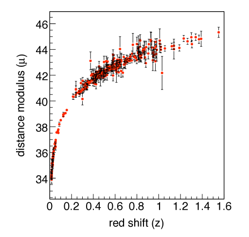
Figure 1: Measurements of $(\mu,z)$ for 307 Type Ia supernovae, compiled by Kowalski et al.

Given a functional relationship between the comoving distance $\chi$ and red shift $z$, the distance modulus function in Eq. (7) can be fitted to the data in Fig. 1 to extract the parameters of the cosmological model. A formula for the comoving distance $\chi$ can be deduced from the FLRW metric, Eq. (2), by noting that light in vacuum travels on null worldlines (for which $ds=0$). Therefore, a light ray from a supernova at red shift $z$ satisfies the relationship $cdt=a(t)d\chi$. Hence,

$$\chi(z) = c\int_{(1+z)^{-1}}^{1}\frac{da}{a\dot{a}},$$ (9)

noting that the light ray was emitted when the scale factor was $a=1/(1+z)$ and received when it assumes the value unity, today.

III A Varying-G Friedmann Equation

Our first assumption, which we have alluded to, is that the universe has zero spatial curvature. Our second assumption is that the Friedmann equation, Eq. (1), for a $K=\Lambda=0$ universe remains valid when $G$ is allowed to vary with time. By valid we mean that the equation is a good approximation to some (unknown) exact equation describing the evolution of the scale factor in a universe in which $G$ varies. This is an example of a conceptual approximation that renders the problem tractable for an undergraduate student. If we wish to remain strictly within the framework of general relativity, we should be cautious about replacing Eq. (1) with one in which $G$ is a function of time because the Friedmann equation is derived from Einstein’s equations

$$G_{\mu\nu}+\Lambda g_{\mu\nu}=\frac{8\pi G}{c^{4}}T_{\mu\nu},$$ (10)

which do not permit variations Barrow in $G$. The tensors $G_{\mu\nu}$ and $T_{\mu\nu}$ are the components of the Einstein and energy-momentum tensors, respectively, and $g$ is the metric tensor. In order to allow for a possible variation of $G$, theories more general than Einstein’s are needed, such as the scalar-tensor theories Barrow ; Berro in which gravity is assumed to couple to a scalar field $\phi$, which—for weak constant coupling—yields the relationship $G\propto\phi^{-1}$. This, in turn, yields a modified Friedmann equation with a time-dependent $G$ and additional terms of order $\dot{G}/G$. If the latter terms are small enough, we obtain a Friedmann equation identical in form to the standard one, but with a time-dependent $G$.

Writing $G(t)=G_{0}f(a)$, where $G_{0}$ is the current value of $G$ and $f(a)$ describes the assumed dependence of $G$ on the scale factor $a(t)$ and therefore cosmic time $t$, and using the definitions

$$\rho_{c0} \equiv 3H_{0}^{2}/8\pi G_{0},$$

$$\rho_{\Lambda} \equiv \Lambda c^{2}/8\pi G_{0},$$

$$\Omega_{M}(a) \equiv \rho(a)/\rho_{c0},$$

$$\Omega_{\Lambda} \equiv \rho_{\Lambda}/\rho_{c0},$$

$$\Omega_{0} \equiv \Omega_{M}(1)+\Omega_{\Lambda},$$ (11)

where $\rho_{c0}$ is the critical density now, $\Omega_{M}(a)$ is the matter density parameter, and $H_{0}$ is the Hubble constant—that is, the value of the Hubble parameter $H(t)\equiv\dot{a}/a$ today, we may write the modified Friedmann equation as

$$\left(\frac{\dot{a}}{a}\right)^{2}=H_{0}^{2}\left[f(a)\Omega_{M}(a)+(1-\Omega_{0})a^{-2}+\Omega_{\Lambda}\right],$$ (12)

noting that

$$-Kc^{2}=H_{0}^{2}(1-\Omega_{0}).$$ (13)

With these definitions, we can write the expressions for the comoving distance $\chi(z)$ and the universal time $t(a)$ as follows,

$$\chi(z)=\frac{c}{H_{0}}\int_{(1+z)^{-1}}^{1}\frac{da}{a^{2}\sqrt{f(a)\Omega_{M}(a)+(1-\Omega_{0})a^{-2}+\Omega_{\Lambda}}},$$ (14)

and

$$t(a)=\frac{1}{H_{0}}\int_{0}^{a}\frac{dx}{x\sqrt{f(x)\Omega_{M}(x)+(1-\Omega_{0})x^{-2}+\Omega_{\Lambda}}}.$$ (15)

The lifetime of the universe is given by $t_{0}=t(1)$.

Our third assumption is that the total mass-energy in the universe, whatever its nature, scales in the same way as matter; that is, we assume that $\Omega_{\Lambda}=0$ and $\Omega_{M}(a)=\Omega_{M0}/a^{3}$, where $\Omega_{M0}=\Omega_{M}(1)$ denotes the value of the matter density parameter today. Since we also assume $K=0$, Eqs. (11) and (13) show that, necessarily, $\Omega_{0}=\Omega_{M0}=1$. However, observations, interpreted within the context of the standard cosmology CMB indicate that the matter density parameter $\Omega_{M0}\approx 0.3$. The difference between $\Omega_{0}=1$ and $\Omega_{M0}$ is presumed to be due to the cosmological constant or dark energy. If we wished to be consistent with this value of $\Omega_{M0}$, while keeping $\Lambda=0$, we need to use a model with $K<0$.

One of our goals, however, is to ascertain whether the SNe data, on their own, are sufficient to conclude that the $\Lambda>0$ model is preferred. To do so, we need merely exhibit another model that works as well. Here we consider varying-G models with $K=\Lambda=0$ and therefore $\Omega_{M0}=1$. Alternatively, one could consider $\Lambda=0$, $K\neq 0$, models. It should be noted, however, that the curvature term $(1-\Omega_{0})a^{-2}$ cannot accelerate the expansion. In a universe dominated by curvature, the Friedmann equation is $\dot{a}=\mbox{constant}$, which implies zero acceleration. To obtain acceleration, one needs a term that dilutes less rapidly than the curvature term, which is the case for a cosmological constant or for the varying-G models described below.

IV Varying-G Models and Results

In principle, a model for the variation of $G$ should arise from some deep theory. Barrow This, however, is far beyond the scope of this paper, which is to give an example of an interesting cosmological study than can be executed in its entirety by an undergraduate physics major, but that nonetheless yields interesting results. We proceed in a purely phenomenological manner. Our basic premise is that the supernovae are further away than expected because gravity was weaker in the past and, consequently, the universe decelerated less rapidly than would be the case were $G$ constant and equal to its current value, $G_{0}$.

IV.1 Fits to Supernovae Data

We studied several forms for the function $f(a)$ in $G(a)=G_{0}f(a)$, but in this paper we report results for only two of them, each with a single adjustable, dimensionless, parameter, $b$. The first varying-G model we studied is defined by

$$f(a)=e^{b(a-1)},\,\,\,\,\mbox{model 1}.$$

In this model, there is no limit to how strong gravity can become. Another model studied is defined by

$$f(a)=2/(1+e^{-b(a-1)}),\,\,\,\,\mbox{model 2},$$

in which $G$ is limited to twice its current value in the distant future. We have normalized both models so that $G(a)$ assumes its current value, $G_{0}$, when $a=1$. For $K=0$ models, the distance modulus, Eq. (7), may be written as

$$\mu(z,b,Q)=5\log_{10}[(1+z)H_{0}\,r(z)/c]+Q,$$ (16)

where the offset $Q$ determines the vertical location of the modulus curve . Note that $H_{0}\,r(z)/c$ is dimensionless and independent of the Hubble constant.

Evaluating Eqs. (14) and (15) for model 1, with $K=0$ (that is, $\Omega_{0}=1$) and $\Omega_{\Lambda}=0$, we find

$$\chi(z)=r(z)=\frac{c}{H_{0}}e^{b/2}\sqrt{2\pi/b}[\mbox{erf}(\sqrt{b/2})-\mbox{erf}(\sqrt{b(1+z)^{-1}/2})],$$ (17)

and

$$t(a)=\frac{1}{H_{0}}[e^{b/2}(\sqrt{2\pi/b}\,\mbox{erf}(\sqrt{ab/2})-2\sqrt{a}\,e^{-ab/2})]/b.$$ (18)

This model exhibits a striking feature: the scale factor becomes infinite in a finite amount of time. We shall return to this point below. For model 2, the integrals in Eqs. (14) and (15) are evaluated numerically using the mid-point rule. 

We fit Eq. (16) to the SNe data in Fig. 1 by minimizing the function

$$\chi^{2}=\sum_{n=1}^{307}[\mu_{n}-\mu(z_{n},b,Q)]^{2}/\sigma_{n}^{2},$$ (19)

with respect to the parameters $b$ and $Q$, where $1\leq n\leq 307$ labels the $n^{\mbox{th}}$ supernova at red shift $z_{n}$ and distance modulus $\mu_{n}$, measured with an uncertainty of $\pm\sigma_{n}$. The minimization of Eq. (19) is done using the program TMinuit, which is part of the ROOT data analysis package from CERN. ROOT For model 1, we get the result shown in Fig. 2.

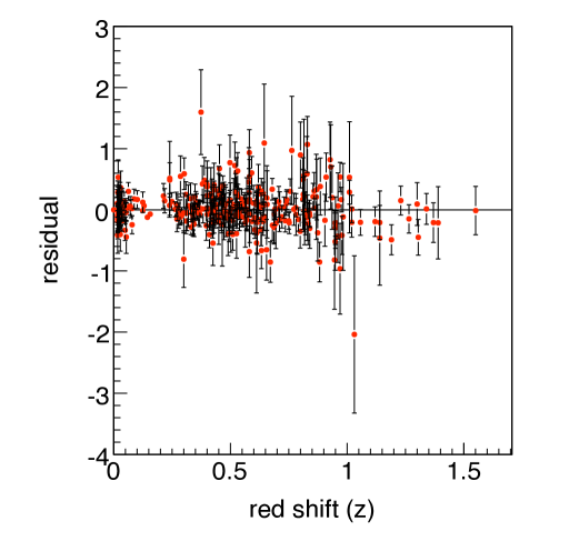
Figure 2: Residuals, $\mu_{n}-\mu(z_{n})$, of fit of model 1 to SNe Ia data ($\chi^{2}/ND=313.0/305=1.03$).

The fit gives the value $b=2.09\pm 0.08$, from which we infer a lifetime of $t_{0}=15.1\pm 0.3$ (70 km s^-1Mpc^-1/$H_{0}$) Gyr.  The fact that the $\chi^{2}$ per degree of freedom ($\chi^{2}/ND)$ is 1.03 suggests that the modulus uncertainties are estimated correctly and that model 1 provides an excellent description of the data.  A similarly good fit is found for model 2, as shown in Fig. 3.

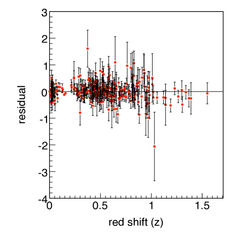
Figure 3: Residuals, $\mu_{n}-\mu(z_{n})$, of fit of model 2 to SNe Ia data ($\chi^{2}/ND=316/305=1.04$).

This fit yields $b=3.27\pm 0.11$, with a $\chi^{2}/ND$ = 316/305 = 1.04. We find $t_{0}=16.2\pm 0.4$ (70 km s^-1Mpc^-1/$H_{0}$) Gyr. For the simplest dark energy model, for which $f(a)=1$ and $\Omega_{M}(a)=(1-\Omega_{\Lambda})/a^{3}$ with $\Omega_{\Lambda}>0$, we find $\Omega_{\Lambda}=0.71\pm.02$ and $t_{0}=14.0\pm 0.3$ (70 km s^-1Mpc^-1/$H_{0}$) Gyr, consistent with the accepted results. DarkEnergy The $\chi^{2}$ per degree of freedom of the fit is 310/305 = 1.02.

Since there is no compelling statistical basis to reject any of these models, we conclude that the supernovae data alone are insufficient to distinguish between them. However, these data when analyzed along with others DarkEnergy are consistent with a simple cosmology in which dark energy mimics a cosmological constant with the value $\Omega_{\Lambda}\approx 0.7$. The varying-G models should likewise be analyzed along with other data to see if a consistent picture emerges. The fact that a $K=\Lambda=0$ model requires $\Omega_{M0}=1$, while the preferred value from galaxy and galaxy cluster measurements is $\Omega_{M0}=0.3$, is already an indication of a difficulty. A systematic analysis of the relevant data, however, is a large task beyond the scope of this paper. Instead, we illustrate the importance of including other data by comparing the predicted fractional variation of $G$, $\dot{G}/G$ at the present epoch, with the available bounds.

IV.2 Bounds on the Variation of $G$

The possible variation of $G$ is usually characterized by the quantity $\dot{G}/G$, which in terms of the logarithmic derivative of the function $f(a)$ is given by

$$\frac{\dot{G}}{G}=\frac{1}{G}\frac{dG}{da}\dot{a}=H_{0}\frac{d\ln f}{da},$$ (20)

where we have used the fact that $H_{0}=\dot{a}/a=\dot{a}$ at the present epoch. Figure 4 shows $\dot{G}/G$ as a function of the scale factor, for models 1 and 2. We see that at $a=1$, $\dot{G}/G$ is equal to $1.5\times 10^{-10}$ y^-1 and $1.15\times 10^{-10}$ y^-1, respectively. Unfortunately, these values for $\dot{G}/G$ are one to three orders of magnitude larger than the upper bounds that range from about $10^{-10}$ y^-1 to $10^{-13}$ y^-1 depending on the method used to extract the bound. GdotG

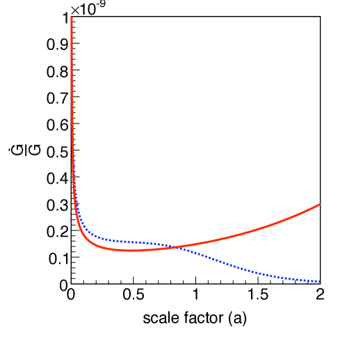
Figure 4: Fractional change in $G$ per year for model 1 (solid curve) and model 2 (dashed curve) as a function of the dimensionless scale factor $a(t)$.

V Discussion and Conclusion

Engaging undergraduate students in research can be an effective way to keep them excited about science. Cosmology is particularly well suited in this regard because it is possible to find topics that are both manageable in scope and scientifically interesting. We have presented an investigation of varying-G cosmological models that serve as examples of interesting research problems that are well matched to the mathematical sophistication of an undergraduate.

The two phenomenological models we presented, in which the strength of gravity increases with cosmic time, provide excellent fits to the Type Ia supernovae data. We therefore conclude that the supernovae data alone cannot establish the dark energy hypothesis unambiguously. Other data are needed to render this hypothesis plausible. However, both our varying-G models fail to satisfy the bounds on $\dot{G}/G$. Consequently, the particular variation of $G$ described by these models is ruled out. In fact, one can make a stronger statement: all varying-G models that give rise to accelerated expansion, and that are based on the FLRW metric and the Friedmann equation, are ruled out by these bounds. Linder Consider, for example, matter-dominated models, for which the Friedmann equation is $H^{2}\sim G/a^{3}\rightarrow G\sim a\dot{a}^{2}$. This yields $\dot{G}/G\sim H+2\ddot{a}/\dot{a}$, from which we conclude that $\dot{G}/G\gtrsim H$. But a value of $\dot{G}/G$ of the order of $H_{0}$ is inconsistent with the bounds on $\dot{G}/G$, which are less than $H_{0}$ by one to three orders of magnitude.

The inability to distinguish between models (model degeneracy) is inherent in the Friedmann equation because the latter is sensitive only to the total energy density of the universe and is agnostic with respect to how the energy density arises. This may be seen by writing the Friedmann equation, Eq. (1), as

$$\left(\frac{\dot{a}}{a}\right)^{2} = \frac{8\pi G}{3}(\rho_{M}+\rho_{K}+\rho_{\Lambda}),$$ (21)

where $\rho_{M}$, $\rho_{K}$, and $\rho_{\Lambda}$ are the density contributions from matter, the curvature and the cosmological constant, respectively. The Hubble parameter $\dot{a}/a$ is related to the sum of $\rho_{M}+\rho_{K}+\rho_{\Lambda}$ not the individual components; or, equivalently, to the sum

$$\Omega\equiv f(a)\Omega_{M}(a)+(1-\Omega_{0})a^{-2}+\Omega_{\Lambda}.$$

Therefore, it is possible to entertain different interpretations of the total energy density. For example, any model based on the Friedmann equation can be reinterpreted as one in which matter, perhaps of several different sorts, is either created, destroyed, or both, as the universe evolves. Consider, for example, the simple cosmological constant dark energy model, for which $f(a)=1$, $\Omega_{0}=1$ and the total energy density is given by $\Omega=(1-\Omega_{\Lambda})/a^{3}+\Omega_{\Lambda}$. This can be rewritten as $\Omega=\Omega_{M}^{\prime}(a)/a^{3}$ with $\Omega_{M}^{\prime}(a)=1-\Omega_{\Lambda}+\Omega_{\Lambda}a^{3}$. Since $a^{-3}$ is the dilution factor for matter, the function $\Omega_{M}^{\prime}(a)$ describes an increasing matter density in a comoving volume, which can be interpreted as the creation of matter as the universe expands! Alternatively, as done here, one can maintain the mass continuity equation, in which case matter is neither created nor destroyed and $\Omega=\Omega_{M0}/a^{3}$, but allow $G$ to vary like $f(a)\sim 1+a^{3}(1-\Omega_{M0})/\Omega_{M0}$. Because of the invariance of the Friedmann equation with respect to such changes in interpretation, it is necessary to impose constraints on the cosmological parameters to remove the model degeneracy. Such constraints can come from other data, or other equations, or both.

It seems odd, at first, that the strengthening of gravity with time leads not to the eventual gravitational collapse of the universe, but rather to its accelerating expansion. The reason for this is that every form of energy contributes to the geometry of spacetime. A model in which the strength of gravity changes with time is equivalent to another model in which the energy density changes in a specific way. If the energy density dilutes more rapidly than $a^{-2}$, then the expansion will slow down. If the strength of gravity increases such that in the equivalent, constant-G model, the energy dilutes more slowly than $a^{-2}$, the expansion will accelerate. In our varying-G models, the effective energy density increases with time.

For model 1, the increasing strength of gravity leads to a startling prediction: a catastrophic end to such a universe. This conclusion follows from the limit $a\rightarrow\infty$ of the lifetime expression, Eq. (18). We find that

$$t(a\rightarrow\infty)=\frac{1}{H_{0}}\exp(b/2)\sqrt{2\pi/b}/b.$$ (22)

According to this model, the universe has a finite lifetime of about 33 Gyr and will tear itself to pieces in its final moments! Such behavior has been dubbed the big rip and is a feature of cosmological models containing phantom energy. bigrip Within regions that are dominated by non-gravitational forces, the effect of a cosmological constant does not change with time and consequently the accelerating universal expansion will not disrupt already bound systems. By contrast, as the universe ages the effect of phantom energy increases in any finite volume of space. Eventually, this precipitates an escalating cascade of destruction at ever smaller scales until everything is torn asunder. We can only hope that phantom energy is just that: a phantom!

References

- (1) See, for example, S. Weinberg, Cosmology (Oxford, New York, 2008), pp. 1–100.
- (2) J. B. Hartle, “General relativity in the undergraduate physics curriculum,” Am. J. Phys. 74, 14–21 (2006).
- (3) See, for example, J. Einasto, “Dark Matter,” arXiv:0901.0632v1 [astro-ph.CO] (2009).
- (4) See, for example, P. J. E. Peebles. B. Ratra, “The Cosmological Constant and Dark Energy,” Rev. Mod. Phys. 75, 559–606 (2003).
- (5) E. V. Linder, “Resource Letter DEAU-1: Dark energy and the accelerating universe,” Am. J. Phys. 76, 197–204 (2008).
- (6) A. G. Riess et al. [The High-Z Team], “Observational Evidence from Supernovae for an Accelerating Universe and a Cosmological Constant,” Astron. J. 116, 1009–1038 (1998).
- (7) S. Perlmutter et al. [The Supernova Cosmology Project], “Measurements of Omega and Lambda from 42 High-Redshift Supernovae,” Astrophys. J. 517, 565–586 (1999).
- (8) J. D. Barrow, “Varying Constants,” Phil. Trans. R. Soc. A 363, 2139–2153 (2005).
- (9) C. J. A. P. Martins, “Cosmology with varying constants,” Phil. Trans. R. Soc. A 360, 2681–2695 (2002).
- (10) M. Kowalski et al., “Improved Cosmological Constraints from New, Old, and Combined Supernova Data Sets,” Astrophys. J. 686, 749–778 (2008).
- (11) R. R. Caldwell, M. Kamionkowski, N. N. Weinberg, “Phantom Energy and Cosmic Doomsday,” Phys. Rev. Lett. 91, 071301 (2003).
- (12) J. C. Wheeler and R. P. Harkness, “Type I supernovae,” Rep. Prog. Phys. 53, 1467–1557 (1990).
- (13) S. Chandrasekhar, An Introduction to the Study of Stellar Structure (Dover, New York, 1967).
- (14) P. Höflich, “Physics of type Ia supernovae,” Nucl. Phys. A 777, 579–600 (2006).
- (15) S. Perlmutter, “Supernovae, Dark Energy, and the Accelerating Universe,” Physics Today, April, 53–60 (2003).
- (16) E. Gaztañaga, E. García-Berro, J. Isern, E. Bravo, and I. Domínguez, “Bounds on the possible evolution of the gravitational constant from cosmological type-Ia supernovae,” Phys. Rev. D 65, 023506 (2001); E. García-Berro, Y. Kubyshin, P. Loren-Aguilar, J. Isern, “The Variation of the Gravitational Constant Inferred from the Hubble Diagram of Type Ia Supernovae,” Int. J. Mod. Phys. D 15, 1163–1174 (2006).
- (17) H. Johnson, W. Morgan, “Fundamental stellar photometry for standards of spectral type on the revised system of the Yerkes spectral atlas,” Astrophys. J., 117, 313–352 (1953).
- (18) Komatsu et al., “Five-Year Wilkinson Microwave Anisotropy Probe Observations: Cosmological Interpretation,” Astrophys. J. Suppl. Ser., 180, 330–376 (2009).
- (19) R. Brun et al., “ROOT,” http://root.cern.ch.
- (20) See for example, J. D. Barrow and P. Parsons, “The Behaviour Of Cosmological Models With Varying-G,” Phys. Rev. D55, 1906–1936 (1997); E. García-Berro, J. Isern, Y. A. Kubyshin, “Astronomical measurements and constraints on the variability of fundamental constants,” Astron. Astrophys. Rev. 14, 113–170 (2007).
- (21) E. V. Linder, private communication.