Fractional Standard Map

Abstract

Properties of the phase space of the standard map with memory are investigated. This map was obtained from a kicked fractional differential equation. Depending on the value of the map parameter and the fractional order of the derivative in the original differential equation, this nonlinear dynamical system demonstrates attractors (fixed points, stable periodic trajectories, slow converging and slow diverging trajectories, ballistic trajectories, and fractal-like structures) and/or chaotic trajectories. At least one type of fractal-like sticky attractors was observed.

1 Introduction

The standard map (SM) can be derived from the differential equation describing kicked rotator. The description of many physical systems and effects (Fermi acceleration, comet dynamics, etc.) can be reduced to the studying of the SM [1]. The SM provides the simplest model of the universal generic area preserving map and it is one of the most widely studied maps. The topics examined include fixed points, elementary structures of islands and a chaotic sea, and fractional kinetics [1, 2, 3].

It was recently realized that many physical systems, including systems of oscillators with long range interaction [4, 5], non-Markovian systems with memory ([6] Ch.10, [7, 8, 9, 10, 11]), fractal media [12], etc., can be described by the fractional differential equations (FDE) [6, 13, 14]. As with the usual differential equations, the reduction of FDEs to the corresponding maps can provide a valuable tool for the analysis of the properties of the original systems. As in the case of the SM, the fractional standard map (FSM), derived in [15] from the fractional differential equation describing a kicked system, is perhaps the best candidate to start a general investigation of the properties of maps which can be obtained from FDEs.

As it was shown in [15], maps that can be derived from FDEs are of the type of discrete maps with memory. One-dimensional maps with memory, in which the present state of evolution depends on all past states, studied previously [16, 17, 18, 19, 20, 21] were not derived from differential equations. Most results were obtained for the generalizations of the logistic map.

In the physical systems the transition from integer order time derivatives to fractional (of a lesser order) introduces additional damping and is similar in appearance to additional friction [6, 22]. Accordingly, in the case of the FSM we may expect transformation of the islands of stability and the accelerator mode islands into attractors (points, attracting trajectories, strange attractors). Because the damping in systems with fractional derivatives is based on the internal causes different from the external forces of friction [22, 23], the corresponding attractors are also different from the attractors of the regular systems with friction and are called fractional attractors [22]. Even in one-dimensional cases [16, 17, 18, 19, 20, 21] most of the results were obtained numerically. An additional dimension makes the problem even more complex and most of the results in the present paper were obtained numerically.

2 FSM, initial conditions

The standard map in the form

$$p_{n+1}=p_{n}-K\sin x_{n},\ \ x_{n+1}=x_{n}+p_{n+1}\ \ ({\rm mod}\ 2\pi)$$ (1)

can be derived from the differential equation

$$\ddot{x}+K\sin(x)\sum^{\infty}_{n=0}\delta\Bigl{(}\frac{t}{T}-n\Bigr{)}=0.$$ (2)

By replacing the second-order time derivative in eq. (2) with the Riemann-Liouville derivative ${}_{0}D^{\alpha}_{t}$ one obtains a fractional equation of the motion in the form

$$_{0}D^{\alpha}_{t}x+K\sin(x)\sum^{\infty}_{n=0}\delta\Bigl{(}\frac{t}{T}-n\Bigr{)}=0,\quad(1<\alpha\leq 2),$$ (3)

where

$${}_{0}D^{\alpha}_{t}x(t)=D^{n}_{t}\ {}_{0}I^{n-\alpha}_{t}x(t)=$$

$$\frac{1}{\Gamma(n-\alpha)}\frac{d^{n}}{dt^{n}}\int^{t}_{0}\frac{x(\tau)d\tau}{(t-\tau)^{\alpha-n+1}}\quad(n-1<\alpha\leq n),$$ (4)

$D^{n}_{t}=d^{n}/dt^{n}$, and ${}_{0}I^{\alpha}_{t}$ is a fractional integral. The initial conditions for (3) are

$$(_{0}D^{\alpha-1}_{t}x)(0+)=p_{1},\\$$

$$(_{0}D^{\alpha-2}_{t}x)(0+)=b.$$ (5)

The Cauchy type problem (3) and (5) is equivalent to the Volterra integral equation of the second kind [24, 25, 26]

$$x(t)=\frac{p_{1}}{\Gamma(\alpha)}t^{\alpha-1}+\frac{b}{\Gamma(\alpha-1)}t^{\alpha-2}$$

$$-\frac{K}{\Gamma(\alpha)}\int^{t}_{0}\frac{\sin[x(\tau)]\sum^{\infty}_{n=0}\delta\Bigl{(}\frac{\tau}{T}-n\Bigr{)}d\tau}{(t-\tau)^{1-\alpha}}.$$ (6)

Defining the momentum as

$$p(t)=\,_{0}D^{\alpha-1}_{t}x(t),$$ (7)

and performing integration in (6) one can derive the equation for the FSM in the form (for the thorough derivation see [26])

$$p_{n+1}=p_{n}-K\sin x_{n},$$ (8)

$$x_{n+1}=\frac{1}{\Gamma(\alpha)}\sum_{i=0}^{n}p_{i+1}V_{\alpha}(n-i+1)+$$

$$\frac{b}{\Gamma(\alpha-1)}(n+1)^{\alpha-2},\ \ \ \ ({\rm mod}\ 2\pi),$$ (9)

where

$$V_{\alpha}(m)=m^{\alpha-1}-(m-1)^{\alpha-1}.$$ (10)

Here it is assumed that $T=1$ and $1<\alpha\leq 2$. The form of eq. (9) which provides a more clear correspondence with the SM ($\alpha=2$) in the case $b=0$ is presented in Sec. 4 (eq. (31)).

The second initial condition in (5) can be written as

$${}_{0}D^{\alpha-2}_{t}(0+)=\lim_{t\rightarrow 0+}\,{}_{0}I^{2-\alpha}_{t}x(t)=$$

$$\lim_{t\rightarrow 0+}\frac{1}{\Gamma(2-\alpha)}\int^{t}_{0}\frac{x(\tau)d\tau}{(t-\tau)^{\alpha-1}}=b,\quad(1<\alpha\leq 2),$$ (11)

which requires $b=0$ in order to have a solution bounded at $t=0$ for $\alpha<2$. The assumption $b=0$ leads to the FSM equations which in the limiting case $\alpha=2$ coincide with the equations for the standard map under the condition $x_{0}=0$.

In this paper the FSM is taken in the form derived in [15] which coincides with (8) and (9) if $b=0$. It is also assumed that $x_{0}=0$ and the results can be compared to those obtained for the SM with $x_{0}=0$ and arbitrary $p_{0}$. As a test, for the SM and for the FSM with $\alpha=2$ and the same initial conditions numerical calculations show that phase portraits look identical.

System of equations (8) and (9) can be considered either in a cylindrical phase space ($x$ mod $2\pi$) or in unbounded phase space. The second case is convenient to study transport. The trajectories in the second case are easily related to the first case. The FSM has no periodicity in $p$ (the SM does) and cannot be considered on a torus.

3 Stable fixed point

The SM has stable fixed points at (0,$2\pi n$) for $K<K_{c}=4$. It is easy to see that point $(0,0)$ is also a fixed point for the FSM. Direct computations using (8) and (9) demonstrate that for the small initial values of $p_{0}$ there is a clear transition from the convergence to the fixed point to divergence when the value of the parameter $K$ crosses the curve $K=K_{c}(\alpha)$ on Fig. 1a from smaller to larger values.

The following system describes the evolution of trajectories near fixed point $(0,0)$

$$\delta p_{n+1}=\delta p_{n}-K\delta x_{n},$$ (12)

$$\delta x_{n+1}=\frac{1}{\Gamma(\alpha)}\sum_{i=0}^{n}\delta p_{i+1}V_{\alpha}(n-i+1).$$ (13)

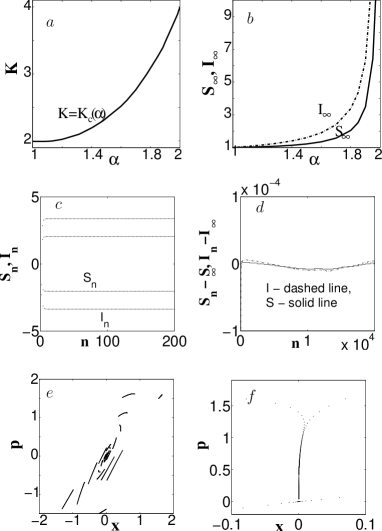
Figure 1: Stability of the fixed point(0,0): a). The fixed point is stable below the curve $K=K_{c}(\alpha)$; b). Values of $S_{\infty}$ and $I_{\infty}$ obtained after 20000 iterations of eqs. (22) and (23). As $\alpha\rightarrow 2$ the values $S_{\infty}$ and $I_{\infty}$ increase rapidly. For $\alpha=1.999$, $S_{\infty}\approx 276$ and $I_{\infty}\approx 552$ after 20000 iterations; c). An example of the typical evolution of $S_{\infty}$ and $I_{\infty}$ over the first 200 iterations for $1<\alpha<2$. This particular figure corresponds to $\alpha=1.8$; d). Deviation of the values $S_{n}$ and $I_{n}$ from the values $S_{\infty}\approx 2.04337$ and $I_{\infty}\approx 3.37416$ for $\alpha=1.8$ during the first 20000 iterations (this type of behavior remains for $1<\alpha<2$); e). Evolution of trajectories with $p_{0}=1.5+0.0005i$, $0\leq i<200$ for the case $K=3$, $\alpha=1.9$. The line segments correspond to the $n$th iteration on the set of trajectories with close initial conditions. The evolution of the trajectories with smaller $p_{0}$ is similar; f). $10^{5}$ iterations on both of two trajectories for $K=2$, $\alpha=1.4$. The one at the bottom with $p_{0}=0.3$ is a fast converging trajectory. The upper trajectory with $p_{0}=5.3$ is an example of the ASCT in which $p_{100000}\approx 0.042$.

The solution can be found in the form

$$\delta p_{n}=p_{0}\sum_{i=0}^{n-1}p_{n,i}\Bigl{(}\frac{2}{V_{\alpha l}}\Bigr{)}^{i}\Bigl{(}\frac{V_{\alpha l}K}{2\Gamma(\alpha)}\Bigr{)}^{i},\quad(n>0),$$ (14)

$$\delta x_{n}=\frac{p_{0}}{\Gamma(\alpha)}\sum_{i=0}^{n-1}x_{n,i}\Bigl{(}\frac{2}{V_{\alpha l}}\Bigr{)}^{i}\Bigl{(}\frac{V_{\alpha l}K}{2\Gamma(\alpha)}\Bigr{)}^{i},\quad(n>0),$$ (15)

The origin of the terms in parentheses, as well as the definition

$$V_{\alpha l}=\sum_{k=1}^{\infty}(-1)^{k+1}V_{\alpha}(k)$$ (16)

will become clear in Sec. 5. Eqs. (12) - (16) lead to the following iterative relationships

$$x_{n+1,i}=-\sum_{m=i}^{n}(n-m+1)^{\alpha-1}x_{m,i-1},\quad(0<i\leq n),$$ (17)

$$p_{n+1,i}=-\sum_{m=i}^{n}x_{m,i-1},\quad(0<i<n)$$ (18)

with the initial and boundary conditions

$$p_{n+1,n}=x_{n+1,n}=(-1)^{n},\quad p_{n+1,0}=1,$$ (19)

$$x_{n+1,0}=(n+1)^{\alpha-1}.$$

From (17) and (18) it is clear that the series (14) and (15) are alternating and it is natural to apply the Dirichlet’s test to verify their convergence. This can be done by considering the totals

$$S_{n}=\sum_{i=0}^{n-1}x_{n,i}\Bigl{(}\frac{2}{V_{\alpha l}}\Bigr{)}^{i},$$ (20)

$$I_{n}=\sum_{i=0}^{n-1}p_{n,i}\Bigl{(}\frac{2}{V_{\alpha l}}\Bigr{)}^{i}.$$ (21)

They obey the following iterative rules

$$S_{n}=n^{\alpha-1}-\frac{2}{V_{\alpha l}}\sum_{i=1}^{n-1}(n-i)^{\alpha-1}S_{i},\quad S_{1}=1,$$ (22)

$$I_{n}=1-\frac{2}{V_{\alpha l}}\sum_{i=1}^{n-1}S_{i}.$$ (23)

Computer simulations show that values of $S_{n}$ and $I_{n}$ converge to the values $(-1)^{n+1}S_{\infty}$ and $(-1)^{n+1}I_{\infty}$ depicted on Fig. 1b. Figs. 1c, 1d show an example of the typical evolution of $S_{n}$ and $I_{n}$ over the first 20000 iterations. It means that the condition of convergence of $\delta p_{n}$ and $\delta x_{n}$ is

$$\frac{V_{\alpha l}K}{2\Gamma(\alpha)}<1.$$ (24)

Numerical evaluation of the equality $K=2\Gamma(\alpha)/V_{\alpha l}$ perfectly reproduces the curve on Fig. 1a obtained by the direct computations of (8) and (9).

Because not only the stability problem (12) and (13), but also the original map (8) and (9), contains convolutions, the use of generating functions [27], which allows transformations of sums of products into products of sums, could be utilized in the investigation of the FSM and some other maps with memory. As an example, in the particular case of the stability problem (12) and (13), the introduction of the generating functions

$$\tilde{W}_{\alpha}(t)=\frac{K}{\Gamma(\alpha)}\sum_{i=0}^{\infty}[(i+1)^{\alpha-1}-i^{\alpha-1}]t^{i},$$ (25)

$$\tilde{X}(t)=\sum_{i=0}^{\infty}\delta x_{i}t^{i},$$ (26)

$$\tilde{P}(t)=\sum_{i=0}^{\infty}\delta p_{i}t^{i},$$ (27)

leads to

$$\tilde{X}(t)=\frac{p_{0}\tilde{W}_{\alpha}(t)}{K}\frac{t}{1-t\Bigl{(}1-\tilde{W}_{\alpha}(t)\Bigr{)}},$$ (28)

$$\tilde{P}(t)=p_{0}\frac{1+\tilde{W}_{\alpha}(t)}{1-t\Bigl{(}1-\tilde{W}_{\alpha}(t)\Bigr{)}}.$$ (29)

Now the original problem is reduced to the problem of the asymptotic behavior at $t=0$ of the derivatives of the analytic functions $\tilde{X}(t)$ and $\tilde{P}(t)$, which is still quite complex and is not considered in this article.

In the region of the parameter space where the fixed point is stable, the fixed point is surrounded by a finite basin of attraction, whose width $W$ depends on the values of $K$ and $\alpha$. For example, for $K=3$ and $\alpha=1.9$ the width of the basin of attraction is $1.6<W<1.7$. Simulations of thousands of trajectories with $p_{0}<1.6$ performed by the authors, of which only 200 (with $1.5<p_{0}<1.6$) are presented in Fig. 1e, show only converging trajectories, whereas among 200 trajectories with $1.6<p_{0}<1.7$ in Fig 2a there are trajectories converging to the fixed point as well as some trajectories converging to attracting slow diverging trajectories (ASDT), whose properties will be discussed in the following section. Trajectories in Fig. 1e converge very rapidly. In the case $K=2$ and $\alpha=1.4$ in addition to the trajectories which converge rapidly and ASDTs there exist attracting slow converging trajectories (ASCT) (Fig. 1f).

4 Attracting slow diverging trajectories (ASDT)

As it can be seen from Fig 2a, the phase portrait on a cylinder of the FSM with $K=3$ and $\alpha=1.9$ contains only one fixed point and ASDTs approximately equally spaced along the $p$-axis. This result corresponds to the fact that the standard map with $K=3$ has only one central island. More complex structure of the standard map’s phase space for smaller values of $K$ (for example for $K=2$ and $K=0.6$) can explain more complex structure of the FSM’s phase space, where periodic attracting trajectories with periods $T=4$ (Fig. 2b), $T=2$, and $T=3$ (Fig. 2c) are present.

Each ASDT has its own basin of attraction (see Fig. 2d). Between those basins two initially close trajectories at first diverge, but then converge to the same or different fixed point or ASDT.

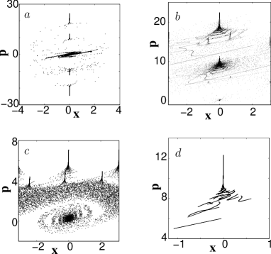
Figure 2: Phase space with ASDTs: a). The same values of parameters as in Fig 1e but $p_{0}=1.6+0.0005i$; b). 200 iterations on trajectories with $p_{0}=4+0.02i$, $0\leq i<500$ for the case $K=2$, $\alpha=1.9$. Trajectories converging to the fixed point, ASDTs with $x=0$, and period 4 attracting trajectories are present; c). 2000 iterations on trajectories with $p_{0}=2+0.04i$, $0\leq i<50$ for the case $K=0.6$, $\alpha=1.9$. Trajectories converging to the fixed point, period 2 and 3 attracting trajectories are present; d).The same values of parameters as in Fig 1e but $p_{0}=5+0.005i$.

Numerical evaluation shows that for ASDTs which converge to trajectories along the $p$-axis ($x\rightarrow x_{lim}=0$) in the area of stability (which is the same as for the stability of the fixed point) the following holds (for large $n$ see Fig. 3a)

$$p_{n}=Cn^{2-\alpha}.$$ (30)

The constant C can be easily evaluated for $1.8<\alpha<2$. Consider an ASDT with $x_{lim}=0$, $T=1$, and $2\pi M$, where $M$ is an integer, constant step in $x$ in the unbounded space. Then Eq. (9) with $b=0$ gives

$$x_{n+1}-x_{n}=\frac{1}{\Gamma(\alpha)}\sum_{k=1}^{n}(p_{k+1}-p_{k})V_{\alpha}(n-k+1)$$ (31)

$$+\frac{p_{1}}{\Gamma(\alpha)}V_{\alpha}(n+1),$$

For large $n$ the last term is small ($\sim n^{\alpha-2}$) and the following holds

$$\sum_{k=1}^{n}(p_{k+1}-p_{k})V_{\alpha}(n-k+1)=2\pi M\Gamma(\alpha).$$ (32)

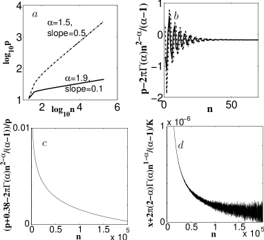
Figure 3: Evaluation of the behavior of the ASDTs: a). Momenta for two ASDTs with $x_{n}\approx 2\pi n$ in the unbounded space (in this example $K=2$). The solid line is related to a trajectory with $\alpha=1.9$ and its slope is 0.1. The dashed line corresponds to a trajectory with $\alpha=1.5$ and its slope is 0.5; b). Deviation of momenta from the asymptotic formula for two ASDTs with $x_{n}\approx 2\pi n$ in the unbounded space, $\alpha=1.9$, and $K=2$. The dashed line has $p_{0}=7$ and the solid one $p_{0}=6$; c). Relative deviation of the momenta for the trajectories in Fig 3b from the asymptotic formula; d). Deviation of the $x$-coordinates for the trajectories in Fig 3b from the asymptotic formula.

With the assumption $p_{n}\sim n^{2-\alpha}$ it can be shown that for values of $\alpha>1.8$ considered the terms in the last sum with large $k$ are small and in the series representation of $V_{\alpha}(n-k+1)$ it is possible to keep only terms of the highest order in $k/n$. Thus, (32) leads to the approximations

$$p_{n}\approx p_{0}+\frac{2\pi M\Gamma(\alpha)n^{2-\alpha}}{\alpha-1},$$ (33)

$$x_{n}\approx-\frac{2\pi M(2-\alpha)\Gamma(\alpha)}{K(\alpha-1)n^{\alpha-1}}.$$ (34)

In the case $K=2$, $\alpha=1.9$ Figs. 3b-3d show two trajectories with $M=1$ (initial momenta $p_{0}=6$ and $p_{0}=7$) approaching an ASDT: the deviation from the asymptotic (33) and (34) and the relative difference with respect to (33).

5 Period 2 stable trajectory

The SM has two stable points of the period $T=2$ trajectory for $4<K<2\pi$ with the property

$$p_{n+1}=-p_{n},\ \ x_{n+1}=-x_{n}.$$ (35)

The same points persist in the numerical experiments for the FSM (Fig 4a). These points are attracting most of the trajectories with small $p_{0}$. Assuming the existence of a $T=2$ attracting trajectory, it is possible to calculate the coordinates of its attracting points $(x_{l},p_{l})$ and $(-x_{l},-p_{l})$. In this case from (8) and (9)

$$p_{l}=\frac{K}{2}\sin(x_{l}),$$ (36)

$$x_{l}=\frac{K}{2\Gamma(\alpha)}\sin(x_{l})\sum_{k=1}^{\infty}(-1)^{k+1}V_{\alpha}(k)$$ (37)

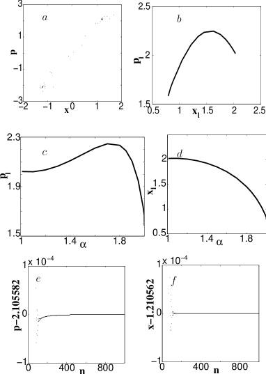
Figure 4: Period 2 stable trajectory: a). An example of $T=2$ attractor for $K=4.5$, $\alpha=1.9$. One trajectory with $x_{0}=0$, $p_{0}=0.513$; b). $p_{l}$ of $x_{l}$ for the case of $K=4.5$; c). $p_{l}$ of $\alpha$ for the case of $K=4.5$; d). $x_{l}$ of $\alpha$ for the case of $K=4.5$; e). $p_{n}-p_{l}$ for the trajectory in Fig. 4a. After 1000 iterations $|p_{n}-p_{l}|<10^{-7}$; f). $x_{n}-x_{l}$ for the trajectory in Fig. 4a. After 1000 iterations $|x_{n}-x_{l}|<10^{-7}$.

Finally, the equation for $x_{l}$ takes the form

$$x_{l}=\frac{K}{2\Gamma(\alpha)}V_{\alpha l}\sin(x_{l}),$$ (38)

where

$$V_{\alpha l}=\sum_{k=1}^{\infty}(-1)^{k+1}V_{\alpha}(k)$$ (39)

and can be easily calculated numerically. From (38) the condition of the existence of $T=2$ trajectory

$$K>K_{c}(\alpha)=\frac{2\Gamma(\alpha)}{V_{\alpha l}},$$ (40)

is exactly opposite to (24). It is satisfied above the curve $K=K_{c}(\alpha)$ on the Fig. 1a. For $\alpha=2$ (40) produces the well-known condition $K>4$ for the SM. The results of calculations of the $x_{l}$ and $p_{l}$ for the cases $K=4.5$, $1<\alpha<2$ presented in Fig. 4b-d perfectly coincide with the results of the direct computations of (8) and (9) with $b=0$. After 1000 iterations presented in Figs. 4e,f the values of deviations $|p_{n}-p_{l}|$ and $|x_{n}-x_{l}|$ are less than $10^{-7}$.

6 Cascade of bifurcations type trajectories (CBTT)

Period 2 stable trajectories have limited basins of attraction. Trajectories that don’t fall into those areas reveal a diverse variety of properties, from period two slow attracting trajectories to fractal type attractors and cascade of bifurcations type trajectories (CBTT).

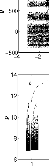
Figure 5: Cascade of bifurcation type trajectories: a). 120000 iterations on a single trajectory with $K=4.5$, $\alpha=1.65$, $p_{0}=0.3$. The trajectory occasionally sticks to a CBTT but then always recovers into the chaotic sea; b). 100000 iterations on a trajectory with $K=3.5$, $\alpha=1.1$, $p_{0}=20$. The trajectory very fast turns into a CBTT which slowly converges to a fractal type area.

Fig. 5a presents a single chaotic trajectory which sticks to the areas similar to the cascade of bifurcations which are well-known for the logistic map. In Fig. 5b a single trajectory falls very rapidly into one of the attracting CBTTs. Because the bifurcation diagram of the logistic map has fractal properties (see for example Chapter 2 in [28]), it is expected that the structure to which this trajectory slowly converges also possesses fractal features.

The properties of this type of attractors, as well as the properties different types of observed during computer simulations chaotic, attracting, and ballistic trajectories for $K>2\pi$ (see Fig 6) will be considered in the subsequent article.

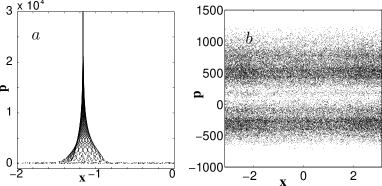
Figure 6: Examples of phase space for $K>2\pi$: a). An attracting ballistic trajectory with $K=6.908745$, $\alpha=1.999$, $p_{0}=0.7$; b). A chaotic trajectory for $K=6.908745$, $\alpha=1.9$.

7 Fractional attractors and their stability

The problems of existence and stability of the fractional attractors for the systems described by the FDEs were addressed in a few recent papers. It was noticed in [22] that the properties of the fractional chaotic attractors are different from the properties of the “regular” chaotic attractors and may have some pseudochaotic features. The problem of existence of multi-scroll fractional chaotic attractors was considered in [29]. The problem of stability of the stationary solutions (fixed points for ODEs) of systems described by the fractional ODEs and PDEs was considered in [30, 31, 32]. In the above mentioned articles the equations contained the Caputo fractional derivatives, whereas in the present article the Riemann-Liouville fractional derivative is used. This fact does not allow a direct comparison of the results. The results [22, 29, 30, 31, 32] were supported by a relatively small number of computations and this is understandable, taking into account all the difficulties of performing numerical simulations for the equations with fractional derivatives.

The use of the FSM, which is equivalent to the original FDE, allows performing thousands of runs of simulations of the kicked fractional system with two parameters: $K$ and $\alpha$. The FSM also allows making some analytic deductions and revealing some properties of the fractional attractors which were not reported before:

a). The stability of the fixed point (0,0) of the FSM is different not only from the stability of the fixed point in the domain of the regular motion (zero Lyapunov exponent) of the SM, but also from the stability of fixed attracting points of the regular (not fractional) dissipative systems like, for example, the dissipative standard map (Zaslavsky map) [33]. The difference is in the way in which trajectories approach the attracting point. In the FSM this way depends on the initial conditions. For example, in Fig. 1f there are two trajectories approaching the same fixed point: one is fast spiraling into the attractor and the other is slowly converging.

b). Stable period 2 attracting trajectories exist only in the asymptotic sense - they do not represent any real periodic solutions. If the initial condition is chosen in a period two stable attracting point, this trajectory will immediately jump out of this point and where it will end depends on the values of $K$ and $\alpha$.

c). All the FSM attractors exist in the sense that there are trajectories which converge into those attractors. But if an initial condition is taken on any of the attracting trajectories (except for the fixed point), they will most likely not evolve along the same trajectory.

8 Conclusion

In this article properties of the phase space of the FSM were investigated. It was shown that islands of regular motion of the SM in the FSM turn into attractors (points, attracting trajectories, and fractal-like structures). Properties of the attracting fixed points, period two trajectories, ASCTs, and ASDTs were considered. This consideration allows the description of the evolution of the dynamical variable $x$ of the original fractional dynamical system, a system described by the FDE reducible to the FSM. Physical interpretation of the momentum, defined through a fractional derivative from the variable $x$, is unclear.

The explanation of the CBTTs, which are interesting phenomena, requires further detailed investigation. Chaotic trajectories that spend some time near CBTTs, which can be called sticky attractors in analogy to sticky islands of the SM, are good candidates for the investigation of anomalous diffusion. Transport was not considered in this article. How general the properties of the phase space of the FSM are will become clear after further investigations of different fractional maps, maps with memory which can be derived from the FDEs, and particular those suggested in [15], will be conducted. The fact that so many physical systems can be reduced to studying of the SM gives a hope that those physical systems which can be reduced to studying the FSM will be found.

References

- [1] B.V. Chirikov, ”A universal instability of many dimensional oscillator systems” Phys. Rep. 52 (1979) 263-379.
- [2] A.J. Lichtenberg, M.A. Lieberman, Regular and Chaotic Dynamics (Springer, Berlin, 1992).
- [3] G.M. Zaslavsky, Hamiltonian Chaos and Fractional Dynamics (Oxford University Press, Oxford, 2005).
- [4] V.E. Tarasov, G.M. Zaslavsky, ”Fractional dynamics of coupled oscillators with long-range interaction” Chaos 16 (2006) 023110.
- [5] V.E. Tarasov, ”Continuous limit of discrete systems with long-range interaction” J. Phys. A. 39 (2006) 14895-14910.
- [6] I. Podlubny, Fractional Differential Equations (Academic Press, San Diego, 1999).
- [7] R.R. Nigmatullin, ”Fractional integral and its physical interpretation” Theoretical and Mathematical Physics 90 (1992) 242-251.
- [8] F.Y. Ren, Z.G. Yu, J. Zhou, A. Le Mehaute, R.R. Nigmatullin, ”The relationship between the fractional integral and the fractal structure of a memory set” Physica A 246 (1997) 419-429
- [9] W.Y. Qiu, J. Lu, ”Fractional integrals and fractal structure of memory sets” Phys. Lett. A 272 (2000) 353-358.
- [10] R.R. Nigmatullin, ”Fractional’ kinetic equations and ’universal’ decoupling of a memory function in mesoscale region” Physica A 363 (2006) 282-298.
- [11] V.E. Tarasov, G.M. Zaslavsky ”Fractional dynamics of systems with long-range space interaction and temporal memory” Physica A 383 (2007) 291-308.
- [12] A. Carpinteri, F. Mainardi, (Eds.), Fractals and Fractional Calculus in Continuum Mechanics (Springer, Wien, 1997).
- [13] S.G. Samko, A.A. Kilbas, O.I. Marichev, Fractional Integrals and Derivatives Theory and Applications (Gordon and Breach, New York, 1993).
- [14] A.A. Kilbas, H.M. Srivastava, J.J. Trujillo, Theory and Application of Fractional Differential Equations (Elsevier, Amsterdam, 2006).
- [15] V.E. Tarasov, G.M. Zaslavsky, ”Fractional equations of kicked systems and descrete maps” J. Phys. A 41 (2008) 435101.
- [16] A. Fulinski, A.S. Kleczkowski, ”Nonlinear maps with memory” Physica Scripta 35 (1987) 119-122.
- [17] E. Fick, M. Fick, G. Hausmann, ”Logistic equation with memory” Phys. Rev. A 44 (1991) 2469-2473.
- [18] K. Hartwich, E. Fick, ”Hopf bifurcations in the logistic map with oscillating memory” Phys. Lett. A 177 (1993) 305-310.
- [19] M. Giona, ”Dynamics and relaxation properties of complex systems with memory” Nonlinearity 4 (1991) 911-925.
- [20] J.A.C. Gallas, ”Simulating memory effects with discrete dynamical systems” Physica A 195 (1993) 417-430; ”Erratum” Physica A 198 (1993) 339-339.
- [21] A.A. Stanislavsky, ”Long-term memory contribution as applied to the motion of discrete dynamical system” Chaos 16 (2006) 043105.
- [22] G.M. Zaslavsky, A.A. Stanislavsky, M. Edelman, ”Chaotic and pseudochaotic attractors of perturbed fractional oscillator” Chaos 16 (2006) 013102.
- [23] A.A. Stanislavsky, “Fractional oscillator” Phys. Rev. E 70 (2004) 051103.
- [24] A.A. Kilbas, B. Bonilla, J.J. Trujillo, ”Nonlinear differential equations of fractional order is space of integrable functions” Doklady Mathematics 62 (2000) 222-226; Translated from Doklady Akademii Nauk 374 (2000) 445-449. (in Russian).
- [25] A.A. Kilbas, B. Bonilla, J.J. Trujillo, ”Existence and uniqueness theorems for nonlinear fractional differential equations” Demonstratio Mathematica 33 (2000) 583-602.
- [26] V.E. Tarasov ”Differential equations with fractional derivative and universal map with memory” Journal of Physics A 42 (2009) 465102.
- [27] W. Feller, An introduction to probability theory and its applications (Wiley, New York, 1968).
- [28] R. Gilmore, M. Lefranc, The Topology of Chaos, Alice in Stretch and Sqeezeland (Wiley, New York, 2002).
- [29] M.S. Tavazoei, M. Haeri, “Chaotic attractors in incommensurate fractional order systems” Physica D 237 (2008) 2628-2637.
- [30] V. Gafiychuk, B. Datsko, V. Meleshko, D. Blackmore, “Analysis of the solutions of coupled nonlinear fractional reaction-diffusion equations” Chaos, Solitons & Fractals 41 (2009) 1095-1104.
- [31] V. Gafiychuk, B. Datsko, “Stability analysis and limit cycle in fractional system with Brusselator nonlinearities” Phys. Let. A 372 (2008) 4902-4904.
- [32] V. Gafiychuk, B. Datsko, V. Meleshko, “Analysis of fractional order Bonhoeffer-van der Pol oscillator” Physica A 387 (2008) 418-424.
- [33] G.M. Zaslavsky, ”Simplest case of a strange attractor” Phys. Let. A 69 (1978) 145-147.