Liquid crystal phases of ultracold dipolar fermions on a lattice

Abstract

Motivated by the search for quantum liquid crystal phases in a gas of ultracold atoms and molecules, we study the density wave and nematic instabilities of dipolar fermions on the two-dimensional square lattice (in the $x-y$ plane) with dipoles pointing to the $z$ direction. We determine the phase diagram using two complementary methods, the Hatree-Fock mean field theory and the linear response analysis of compressibility. Both give consistent results. In addition to the staggered ($\pi$, $\pi$) density wave, over a finite range of densities and hopping parameters, the ground state of the system first becomes nematic and then smectic, when the dipolar interaction strength is increased. Both phases are characterized by the same broken four-fold (C₄) rotational symmetry. The difference is that the nematic phase has a closed Fermi surface but the smectic does not. The transition from the nematic to the smectic phase is associated with a jump in the nematic order parameter. This jump is closely related to the van Hove singularities. We derive the kinetic equation for collective excitations in the normal isotropic phase and find that the zero sound mode is strongly Landau damped and thus is not a well defined excitation. Experimental implications of our results are discussed.

I Introduction

It is well known that as the strength of Coulomb interaction is increased with respect to the kinetic energy, an electron gas goes from a liquid state to a crystalline phase Wigner (1934). However the transition from a liquid to a crystal phase in fermionic systems with long range interaction may contain several intermediate stages bearing the name of “electronic liquid crystal” phases  Fradkin et al. (2007). Analogous to the classical liquid crystals Chaikin and Lubensky (1995), these phases are classified as being “nematic” and “smectic” according to their symmetry breaking (Fermi surface deformation) as compared to the isotropic case. In the nematic phase Kivelson et al. (1998); Yamase and Kohno (2000a); Oganesyan et al. (2001); Kee et al. (2003); Khavkine et al. (2004); Quintanilla and Schofield (2006), the rotational symmetry is broken so the typical Fermi surface has a cigar-like shape, i.e., it is stretched in one direction and shrunk in other directions. In the smectic phase the system is effectively in a reduced dimension Kivelson et al. (1998), accordingly the Fermi surface is divided into disconnected pieces. The transition to the smectic phases is thus naturally connected to dimensional crossover phenomena which have drawn many interests Carlson et al. (2000); Biermann et al. (2001); Ho et al. (2004); Kollath et al. (2008).

Electronic nematic order has been observed and studied in a number of solid state materials, such as transition metal oxides Tranquada et al. (1995); Orenstein and Millis (2000); Yamase and Kohno (2000b); Kivelson et al. (2004) and quantum Hall systems (e.g., GaAs/AlGaAs heterostructure in high magnetic field) Lilly et al. (1999); Pan et al. (1999). These systems are typically two-dimensional and signatures of nematic order include additional peaks in neutron scattering Tranquada et al. (1995) and transport anisotropy Lilly et al. (1999); Borzi et al. (2007). The nematic order can be viewed either as fluctuations (disordering) of static stripe-like ordered states Sun et al. (2008) or as an instability of the liquid (isotropic) states Lawler et al. (2006). Possible nematic order in the two-dimensional Hubbard model has been extensively discussed in the context of high temperature superconductors Tranquada et al. (1995); Yamase and Kohno (2000b); Halboth and Metzner (2000). Away from half filling, a stripe order can be stabilized by the antiferromagnetic (AF) spin exchange. For example, at $1/8$ doping, three quarters of sites have one localized electron with AF spin arrangement maximizing the energy gain from spin-exchange, while the rest one quarter of sites have an average 0.5 delocalized electron propagating along one particular direction forming “conducting veins”; these conducting veins appear every four lattice constants constituting the stripe phase Tranquada et al. (1995); Orenstein and Millis (2000). The nematic order can thus be viewed as quantum and/or thermal fluctuations of these static stripes Kivelson et al. (1998); Lawler et al. (2006). Similar understanding applies to quantum Hall systems as well Koulakov et al. (1996); Fradkin and Kivelson (2009).

Because of their excellent tunability with dipole moments, cold polar molecular gases have been proposed as an ideal system to study the electronic liquid crystal phases Mancini et al. (2004); Buchler et al. (2007); Micheli et al. (2007); Sawyer et al. (2007); Ni et al. (2008). Under an external electric or magnetic field, all dipoles are aligned along the field direction, and the potential energy between two dipoles is $V(\vec{R})=d^{2}[1-3\cos^{2}\theta]/|\vec{R}|^{3}$, with $d$ the induced dipole moment, $\vec{R}$ the relative position between the two dipoles, and $\theta$ the angle between the applied field and $\vec{R}$. Since the induced dipole moment is proportional to the external field, by tuning the amplitude and the angle (relative to the system) of the field one can directly control the strength of long-range interaction. Recently, there appeared many theoretical works on dipolar Fermi gas in the continuum Miyakawa et al. (2008); Fregoso et al. (2009); Chan et al. (2009); Fregoso and Fradkin (2009); Baranov et al. (2004); Bruun and Taylor (2008); Zhao et al. (2009). By contrast, studies on dipolar fermions on lattices are relatively few and focus on anisotropic lattices Quintanilla et al. (2009).

In this paper we consider the simplest possible system where a single species of dipolar fermions are loaded into the square optical lattice (in the $x-y$ plane) Yamase et al. (2005) with the external field along the $z$ direction, schematically shown in Fig. 1(a). In this setup the dipolar interaction has the simple form $d^{2}/R^{3}$. We focus on the instabilities of the normal isotropic phase. We find that the transitions from isotropic to liquid crystal phases are generally of first order. The transitions to smectic phase are associated with a jump in the order parameter which is closely related to the van Hove singularities in the low dimensional lattices Halboth and Metzner (2000); Hankevych et al. (2002). Our estimate shows that the magnitude of dipole moment required to achieve the liquid crystal phases is within the reach of current experiments of hetero-nuclear polar molecules. The rest of the paper is organized as follows. In section II, we introduce our model Hamiltonian and define all relevant phases. We also discuss the van Hove points in this model and the special features of dipolar scattering between them. In Section III, we analyze in detail the various instabilities from the isotropic state to obtain the phase diagram of the system. This is done by Hatree-Fock mean field theory and linear response analysis of the compressibility. Special attention is paid to understand the order of normal-nematic and nematic-smectic transitions. In section IV we study the collective excitations in the isotropic phase. We briefly discuss the implications of our results to experiments in section V before conclude in section VI.

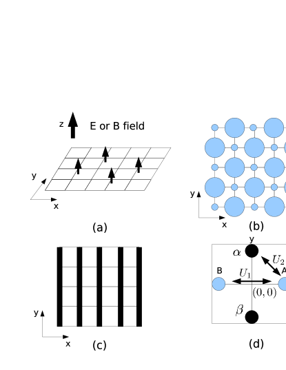
Figure 1: (a) The experimental setup: a square lattice in the $x-y$ plane and the applied field (either electric or magnetic) along the $z$ direction. The dipole moments of fermions are aligned along the $z$ direction which leads to large intersite density-density interaction. (b) The staggered density wave: the density is more concentrated on one sublattice than the other. The size of circle indicates the density at the given site. (c) The nematic phase: the effective hoppings along $x$ and $y$ are different. (d) The first Brillouin zone of the square lattice. Four circles ($A,B,\alpha,\beta$) mark the regions near the van Hove points. The interaction between the opposite van Hove points is $U_{1}$, and for neighboring van Hove points is $U_{2}$.

II Model and definition

The general Hamiltonian for single species of dipolar fermions on the square lattice is

$$H = \sum_{ij}t_{ij}\hat{c}^{\dagger}_{i}\hat{c}_{j}+\frac{1}{2}\sum_{ij}V_{ij}\hat{n}_{i}\hat{n}_{j}-\mu\sum_{i}\hat{n}_{i},$$ (1)

$$= \sum_{\vec{k}}(\epsilon_{\vec{k}}-\mu)\hat{c}^{\dagger}_{\vec{k}}\hat{c}_{\vec{k}}+\frac{1}{N}\sum_{\vec{k}}V(\vec{k})\hat{\rho}_{\vec{k}}\hat{\rho}_{-\vec{k}}.$$

Here, $t_{ij}$ is the hopping amplitude between site $i$ and $j$, $V_{ij}\propto d^{2}/|\vec{r}_{i}-\vec{r}_{j}|^{3}$ is the (repulsive) dipolar interaction between site $i$ and $j$, $V(\vec{k})$ is the Fourier transform of $V_{ij}$, $N$ is the total number of sites, $\epsilon_{\vec{k}}$ is the bare (in the absence of $V_{ij}$) band energy dispersion, and $\hat{\rho}_{\vec{k}}=\sum_{\vec{q}}\hat{c}^{\dagger}_{\vec{q}+\vec{k}}\hat{c}_{\vec{q}}$. Since the intersite repulsion takes the form of density-density interaction, this model is sometimes referred to as the extended Hubbard model Nayak (2000). The actual calculation is done for a given density (particle per site) $n$, and the chemical potential $\mu$ is adjusted to yield the fixed density.

First we give the precise definitions of several phases in our system. Due to the presence of lattice, the “isotropic” or normal phase is a state that has the same symmetry of the Hamiltonian. In the nematic phase, the C₄ rotation symmetry is reduced to C₂ but the lattice translational symmetry still holds in both the $x$ and $y$ direction. A further constraint is that the Fermi surface is closed. On the mean field level, the nematic phase can be viewed as the effective hopping amplitudes (renormalized by the dipolar interaction) along the $x$ and $y$ direction are different, as demonstrated in Fig. 1(c). The transition from the isotropic to the nematic phase is also referred to as Pomeranchuk instability  Halboth and Metzner (2000); Pomeranchuk (1958). The smectic phase has the same symmetry as the nematic, but has an open Fermi surface. The transition from the nematic to the smectic phase is a Lifshitz transition Abrikosov (1988) where the topology of Fermi surface changes. Finally, we also consider the possibility of the staggered density wave (sDW) phase, in which the average density on one sublattice is different from the other sublattice, as illustrated in Fig. 1(b).

Compared to the continuum gas, an important feature of the two dimensional lattice is the van Hove singularity in the density of states. The van Hove points ($\vec{k}_{VH}$) are $\vec{k}$-points in the reciprocal space with vanishing group velocity $\vec{\nabla}_{\vec{k}}\epsilon_{\vec{k}}|_{\vec{k}=\vec{k}_{VH}}=0$. In two-dimension, this leads to a logarithmic divergence in the density of states, i.e. the density of states $g(\varepsilon)\sim-\log|\varepsilon-\varepsilon_{VH}|$ where $\varepsilon_{VH}=\epsilon_{\vec{k}_{VH}}$ is the van Hove energy. The lattice symmetry implies that for a non-zero $\vec{k}_{VH}$, all other $\vec{k}$ points generated by symmetry transformations of $\vec{k}_{VH}$ are also van Hove points. When the chemical potential is close to $\varepsilon_{VH}$, most low energy excitations are around $\vec{k}_{VH}$, so interactions between states near the van Hove points become dominantly important.

Our subsequent discussion will be valid for the general form of the Hamiltonian Eq. (1). In the numerical simulation, however, we choose a specific Hamiltonian as follows. We keep the first and second nearest neighbor hopping $t$ and $t^{\prime}$, which gives $\epsilon_{\vec{k}}=-2t(\cos k_{x}+\cos k_{y})-4t^{\prime}\cos k_{x}\cos k_{y}$. Since the strength of dipolar interaction falls off rapidly as a function of distance ($1/r^{3}$), we consider the case where the lattice constant is large enough so that only the nearest neighbor density-density interaction is kept Quintanilla et al. (2009). Under this simplification the dipolar interaction strength is described by a single parameter $U$ ($>$0), i.e., in Eq. (1) $V_{ij}=(U/2)\delta_{i,j\pm\hat{a}}$ with $\hat{a}=\hat{x}$ or $\hat{y}$ and $V(\vec{k})=+U/2(\cos k_{x}+\cos k_{y})$. The specific model is thus parametrized by the hopping $t$ and $t^{\prime}$, the dipolar interaction strength $U$, and the filling (density) $n$. All energies are measured in unit of $t$ for the remaining discussion. For this model, the van Hove points are located at $(0,\pm\pi)$ and $(\pm\pi,0)$. They are labeled by $A,B$ and $\alpha,\beta$, respectively as shown in Fig. 1(d). As we shall explicitly show in next section (the discussion below Eq. (7)), $-2V(\vec{k}-\vec{k}^{\prime})$ is identified as the interaction between states labeled by $\vec{k}$ and $\vec{k}^{\prime}$. We point out here that the dipolar interaction between opposite van Hove points (such as $A$ and $B$ in Fig. 1(d)) is attractive,

$$U_{1}\equiv-2V(\vec{k}-\vec{k}^{\prime})|_{\vec{k}=(-\pi,0),\vec{k}^{\prime}=(\pi,0)}=-2U,$$ (2)

while it is repulsive between neighboring van Hove points (such as $A$ and $\alpha$ in Fig. 1(d)),

$$U_{2}\equiv-2V(\vec{k}-\vec{k}^{\prime})|_{\vec{k}=(0,\pi),\vec{k}^{\prime}=(\pi,0)}=+2U.$$ (3)

This property of dipolar interaction is very important for our discussion of the nematic instability in the next section.

III Phase diagram

First, we use Hartree-Fock (HF) approximation to study the ground state of the system Eq. (1) at zero temperature. HF mean field theory has been playing an important role in previous studies of electronic nematic phases Kee et al. (2003); Quintanilla and Schofield (2006); Quintanilla et al. (2009). We consider and compare two possible symmetry breaking phases: the staggered density wave and the nematic phase. We have also considered the $d$-density wave state Nayak (2000); DDW but found it has higher energy than the staggered density wave (also known as $s$-density wave in Ref. Nayak (2000)), so we shall not discuss it in any detail here.

Staggered Density Wave (sDW): In this phase, the fermion density is more concentrated on one of the square sublattices as shown in Fig. 1(b), so $\langle\rho_{\vec{Q}}\rangle$ is nonzero with $\vec{Q}=(\pi,\pi)$. This arrangement can reduce the nearest neighbor repulsion energy, which is the dominant interaction energy. Within the HF approximation, the reduced Hamiltonian for this phase is simply

$$H_{HF}^{sDW}= \sum_{\vec{k}}(\epsilon_{\vec{k}}-\mu)\hat{c}^{\dagger}_{\vec{k}}\hat{c}_{\vec{k}}+2V(\vec{Q})M_{sDW}\hat{\rho}_{\vec{Q}}$$

$$-NV(\vec{Q})M_{sDW}^{2}.$$ (4)

Here, the sDW order parameter $M_{sDW}$ is given by the self-consistent equation $\frac{\partial\langle H_{HF}^{sDW}\rangle}{\partial M_{sDW}}=0$,

$$M_{sDW}=\frac{1}{N}\sum_{\vec{k}}\langle\hat{c}^{\dagger}_{\vec{k}+\vec{Q}}\hat{c}_{\vec{k}}\rangle.$$ (5)

By solving Eq. (4) and (5), one can obtain the critical interaction strength $U_{c}$ above which $M_{sDW}$ becomes nonzero.

Nematic phase: In the nematic phase, the system has to rotate $180^{\circ}$, instead of $90^{\circ}$, to go back to itself. To understand the basic mechanism behind the spontaneous Fermi surface distortion (which costs kinetic energy), we count the interaction energy between all four van Hove points. As shown in Fig. 1(d) and discussed above, the interaction between opposite van Hove points is $U_{1}$ while between neighboring points is $U_{2}$. The total interaction energy is

$$E_{tot}=U_{1}(n_{A}n_{B}+n_{\alpha}n_{\beta})+U_{2}(n_{A}+n_{B})(n_{\alpha}+n_{\beta}).$$

In the isotropic phase, $n_{A}=n_{B}=n_{\alpha}=n_{\beta}=n_{0}$, leading to

$$E^{iso}_{tot}=E_{0}=(2U_{1}+4U_{2})n_{0}^{2}.$$

In the nematic phase, quite generally we have $n_{A}=n_{B}=n_{0}-\delta$, $n_{\alpha}=n_{\beta}=n_{0}+\delta$, where $\delta$ characterizes the distortion. This leads to total interaction energy

$$E^{nem}_{tot}=E_{0}+(2U_{1}-4U_{2})\delta^{2}.$$

Therefore if $U_{1}<0$ and $U_{2}>0$, which we have shown is exactly the case for dipolar interaction in Eq. (2) and (3), the nematic phase is energy favored over the isotropic phase with net energy gain

$$\Delta E=(2|U_{1}|+4|U_{2}|)\delta^{2}>0.$$

Similar argument was elaborated by Halboth and Metzner Halboth and Metzner (2000) in the context of the two-dimensional Hubbard model away from half filling. There, the effective interactions between van Hove points come from a renormalization procedure, while in the present case, the required interactions come directly from the dipolar interaction.

To formulate a HF description of the nematic phase, we notice that because of the lattice translational symmetry, the crystal momentum is still a good quantum number and the nematic state can be described by a distribution function $n_{\vec{k}}=\Theta(\tilde{\mu}-\tilde{\epsilon}_{\vec{k}})$ Quintanilla et al. (2009); Quintanilla and Schofield (2006) where $\tilde{\epsilon}_{\vec{k}}$ is the renormalized dispersion to be specified and $\tilde{\mu}$ is the corresponding chemical potential determined by the fermion density. With this ansatz, the Hartree-Fock Hamiltonian for the nematic phase is

$$H_{HF}^{nem}= \sum_{\vec{k}}(\tilde{\epsilon}_{\vec{k}}-\tilde{\mu})\hat{c}^{\dagger}_{\vec{k}}\hat{c}_{\vec{k}}-NV(0)n^{2}$$

$$+\frac{1}{N}\sum_{\vec{k}\vec{k}^{\prime}}V(\vec{k}-\vec{k}^{\prime})n_{\vec{k}}n_{\vec{k}^{\prime}},$$ (6)

with $\tilde{\mu}=\mu-2V(0)n$ and

$$\tilde{\epsilon}_{\vec{k}}(\{n_{\vec{k}}\})=\epsilon_{\vec{k}}-\frac{2}{N}\sum_{\vec{k}^{\prime}}V(\vec{k}-\vec{k}^{\prime})n_{\vec{k}^{\prime}}.$$ (7)

Note that $n_{\vec{k}}$ (or equivalently $\tilde{\epsilon}_{\vec{k}}$) has to be solved self-consistently from Eq. (6) and Eq. (7). From Eq. (6), $-2V(\vec{k}-\vec{k}^{\prime})$ is identified as the interaction between quasi-particles with momentum $\vec{k}$ and $\vec{k}^{\prime}$. For calculations with fixed density, the Hartree term $2V(0)n$ is independent of $\vec{k}$ and only shifts the chemical potential by a constant, therefore for simplicity we denote the chemical potential with $\mu$ (instead of $\tilde{\mu}$) in following discussions. The nematic order parameter $M^{nem}$ can be defined as

$$M^{nem}=\frac{8}{N}\sum_{0<k_{x}<k_{y}<\pi}(\tilde{\epsilon}_{k_{x},k_{y}}-\tilde{\epsilon}_{k_{y},k_{x}}).$$ (8)

Note the summation is restricted in the first quadrant of the Brillouin zone and only for $k_{x}<k_{y}$, because parity is conserved in the nematic phase. One notes that the formalism described here applies to the smectic phase.

III.1 Phase boundaries

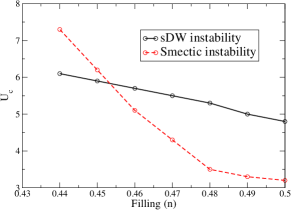
Figure 2: The phase boundaries of staggered density wave (solid) and smectic phase (dashed) for $t^{\prime}=0$, $n=0.44-0.5$. The ordered quantum phase is above the respective transition line.

For given $t^{\prime}$ and $n$, we first compute the critical interaction strength $U_{c}$ for both the staggered density wave and the nematic or smectic phase. Whichever has a smaller $U_{c}$ is identified as the leading instability of the system. For example Fig. 2 shows $U_{c}$ for both phases as a function of $n$ for $t^{\prime}=0$. For these parameters the smectic phase is the leading instability when $0.46<n<0.5$, while staggered density wave is the leading stability for $n<0.46$. Table I summarizes the results for several $t^{\prime}$ and fillings $n$. We found when $t^{\prime}$ is negative enough and the filling is not too close to the van Hove points, the system first undergoes a weakly $first$ order transition to the nematic phase before entering the smectic phase.

	sDW	Nematic	Smectic
$t^{\prime}=0$	$n<0.46$	no	0.46-0.5
$t^{\prime}=-0.1$	$n<0.43$	no	0.43-0.47
$t^{\prime}=-0.2$	$n<0.39$	0.39-0.41	0.41-0.45
$t^{\prime}=-0.3$	$n<0.36$	0.36-0.38	0.38-0.4

Table I: The leading instability for $t^{\prime}=0$, -0.1, -0.2, -0.3 and $n<0.5$.

III.2 The order parameter

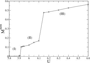
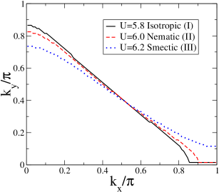
Figure 3: (a) The nematic order parameter as a function of $U$. (b) The Fermi surface in the first quadrant of the Brillouin zone for $U=5.8$ (isotropic), 6 (nematic), and 6.2 (smectic). These results are computed at $t^{\prime}=-0.2$ and $n=0.4$.

Fig. 3(a) shows the general behavior of nematic order parameter $M^{nem}$ as a function of $U$, computed for $t^{\prime}=-0.2$ and $n=0.4$. The interaction strength $U$ can be divided into three regions. For small $U$ (Region I), the system is isotropic as indicated by the Fermi surface for $U=5.8$ (solid curve) in Fig. 3(b). When $U>U_{c}^{nem}\sim 5.9$ (Region II), the symmetry between the $x$ and $y$ direction is broken, the systems enters the nematic phase, and the corresponding Fermi surface, elongated in the $x$ direction, is shown (dashed curve) in Fig. 3(b) for $U=6.0$. We emphasize that the isotropic-nematic phase transition is of weakly first order. Finally, when $U>U_{c2}\sim 6.15$ (Region III), there is another jump in the order parameter corresponding to a Lifshitz transition into the smectic phase. The open Fermi surface for $U=6.2$ is shown (dot line) in Fig. 3(b). This transition is also referred to as the meta-nematic transition which emphasizes the the jump between non-zero values of the order parameter Quintanilla et al. (2009); Yamase (2007). We also note that if the filling is such that the Fermi surface is too close to the van Hove points or the second nearest neighbor hopping $t^{\prime}$ is not negative enough (e.g. the first two rows of Table I), the nematic region II disappears and the system undergoes a first order transition directly to the smectic phase. In the following we discuss in more details about these two transitions.

III.3 The isotropic to nematic transition

The transition to the liquid crystal phases was shown previously to be first order for lattice systems Oganesyan et al. (2001); Kee et al. (2003). Following the argument of Ref. Oganesyan et al. (2001), one can expand the ground state energy in terms of the order parameter $Q$ as

$$E(Q)=E(0)+\frac{A}{4}Q^{2}+\frac{B}{8}Q^{4}+\cdots.$$ (9)

The coefficient $B$ is proportional to the cubic correction to the linearized dispersion around the Fermi momentum which is generally negative for realistic band structures Oganesyan et al. (2001); Kee et al. (2003). For example, for the tight-binding band we consider here $\epsilon(\vec{k})=-2t(\cos k_{x}+\cos k_{y})-4t^{\prime}\cos k_{x}\cos k_{y}$, the cubic term in the expansion of $\epsilon(\vec{k}_{f}+(q,0))-\epsilon(\vec{k}_{f})$ in $q$ with $\vec{k}_{f}=(\alpha,0)$ is proportional to $-(t+2t^{\prime})\sin\alpha$ which is normally negative ($2|t^{\prime}|<t$). Negative $B$ makes the isotropic-nematic transition first order. In this case the nematic phase is expected to be stabilized by the higher power term of $Q$ in the energy, for example $Q^{6}$.

If $\vec{k}_{f}$ is too close to the van Hove points, the system undergoes phase transition directly from the isotropic to the smectic phase. On the other hand, if $\vec{k}_{f}$ is far away enough from van Hove points and $t^{\prime}$ is negative enough to reduce the quartic contribution (make $|B|$ smaller), there is a finite window for stable nematic phase. For the model considered here we found $t^{\prime}$ has to be smaller than $-0.2t$ for the nematic phase to occur.

III.4 The linear response analysis

To analyze the Fermi surface instability in more detail, we consider the response $\delta n_{\vec{k}}$ caused by a Fermi surface perturbation $d\mu_{\vec{k}}$ Nozi$\grave{e}$res and Pines (1999); Lamas et al. (2008). The perturbation $d\mu_{\vec{k}}$ modifies the effective dispersion from $\tilde{\epsilon}_{\vec{k}}$ to $\tilde{\epsilon}^{\prime}_{\vec{k}}$. To the linear order of $d\mu_{\vec{k}}$, the change $\tilde{\epsilon}^{\prime}_{\vec{k}}-\tilde{\epsilon}_{\vec{k}}=\gamma d\mu_{\vec{k}}$. Accordingly,

$$\delta n_{\vec{k}} =-\delta(\tilde{\epsilon}_{\vec{k}}-\mu)[\tilde{\epsilon}^{\prime}_{\vec{k}}-\tilde{\epsilon}_{\vec{k}}-d\mu_{\vec{k}}]$$

$$=+\delta(\tilde{\epsilon}_{\vec{k}}-\mu)\times(1-\gamma)d\mu_{\vec{k}}.$$ (10)

We define the momentum-dependent compressibility as $\kappa(\vec{k})=\delta n_{\vec{k}}/d\mu_{\vec{k}}=+\delta(\tilde{\epsilon}_{\vec{k}}-\mu)\times(1-\gamma)$. A stable Fermi surface has positive compressibility ($1-\gamma>0$). We have assumed that $\gamma$ is $k$-independent despite the presence of lattice. The validity of this assumption will be established shortly. Using Eq. 7, one finds

$$\tilde{\epsilon}^{\prime}_{\vec{k}}-\tilde{\epsilon}_{\vec{k}}=-\frac{2}{N}\sum_{\vec{k}^{\prime}}V(\vec{k}-\vec{k}^{\prime})\delta(\tilde{\epsilon}_{\vec{k}^{\prime}}-\mu)(1-\gamma)d\mu_{\vec{k}^{\prime}}.$$ (11)

This equation, combined with the definition of $\gamma$, leads to the eigenvalue equation

$$\sum_{\vec{k}^{\prime}}c_{\vec{k}\vec{k}^{\prime}}d\mu_{\vec{k}^{\prime}}=\lambda d\mu_{\vec{k}},$$ (12)

with $\lambda=\frac{\gamma}{1-\gamma}$ and $c_{\vec{k}\vec{k}^{\prime}}=-\frac{2}{N}V(\vec{k}-\vec{k}^{\prime})\delta(\tilde{\epsilon}_{\vec{k}^{\prime}}-\mu)$. $1-\gamma>0$ translates to $\lambda>-1$, so the condition for stable Fermi surface becomes Det$(c_{\vec{k}\vec{k}^{\prime}}+1)>0$. The delta function in the definition of matrix $c_{\vec{k}\vec{k}^{\prime}}$ has to be treated with care in numerical calculations, this is discussed in the Appendix.

We first discuss the implications and limitations of Eq. (12). First, in the eigenvalue equation, the eigenvector $\{d\mu_{\vec{k}}\}$ corresponding to the eigenvalue approaching $\lambda=-1$ provides information about the shape of Fermi surface in the nematic phase. Second, $c_{\vec{k}\vec{k}^{\prime}}$ contains a $\delta$ function, indicating that only $k$ points at the Fermi surface defined by the renormalized $\tilde{\epsilon}_{\vec{k}}$ are relevant. As explicitly shown in the appendix, the $\delta$ function further implies that the main contribution is from $\vec{k}$ points whose renormalized Fermi velocities $|\vec{\nabla}\tilde{\epsilon}_{\vec{k}}|$ are smallest, i.e. where the dispersion is flat and there are plenty of states with energies close to $\mu$. Those points are related by lattice symmetry operations (rotations and reflections). When applying Eq. (12) to determine the instability, the weak $\vec{k}$ dependence of $\gamma$ can be safely ignored. Finally, Eq. (12) fails due to divergences when the Fermi surface crosses the van Hove points. It also becomes inapplicable if the phase transition is of first order.

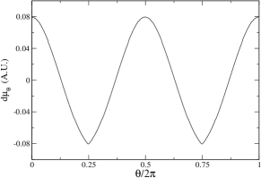
Figure 4: The eigenvector of the softest mode of Eq. (12) computed for $U=5.8$, $t^{\prime}=-0.2$, and $n=0.4$.

Because the transition is only of weakly first order, we apply Eq. (12) to analyze the transition between the isotropic (Region I) and the nematic (Region II) phase. First, the nematic instability can be detected by the emergence of negative eigenvalue of matrix $(c_{\vec{k}\vec{k}^{\prime}}+I)$, where $I$ is the identity matrix. We find that for the nematic transition, which we find is of weakly first order, the critical value $U_{c}^{nem}$ obtained by the Hartree-Fock approximation is roughly $5\%$ smaller than that by analysis using Eq. (12). Actually even for the isotropic-smectic transition, $U_{c}^{smec}$ from Eq. (12) is found to be just roughly $10\%$ larger than the mean field result. Since the Hartree-Fock calculation converges very slowly near the transition, it is of advantage to determine $U_{c}$ from the linear response analysis presented here. Second, the eigenvector of the softest mode, i.e., the one corresponding to the smallest eigenvalue of $c_{\vec{k}\vec{k}^{\prime}}+I$ in Eq. (12), tells how the Fermi surface deforms in the nematic phase. Fig. 4 shows the softest eigenmode $d\mu_{\theta}$ for $U=5.8$, $t^{\prime}=-0.2$, and $n=0.4$, where the angle $\theta\equiv\tan^{-1}\frac{k_{y}}{k_{x}}$ in the polar coordinate. Here $d\mu_{\theta}$, the perturbative deformation of the Fermi surface, is consistent with the Fermi surface in the nematic phase obtained in HF calculation, the dashed curve in Fig. 3(b).

III.5 The meta-nematic transition

The order parameter jump across the nematic-to-smectic or isotropic-to-smectic transition is also closely related to the van Hove singularities. The Fermi surface is defined by $\tilde{\epsilon}_{\vec{k}}=\mu$. For a given direction, the change in Fermi momentum $\triangle k_{F}$ due to a change in the chemical potential $\triangle\mu$ is proportional to $\frac{\triangle\mu}{|\vec{\nabla}_{\vec{k}}\tilde{\epsilon}|}$. Because the area enclosed by the Fermi surface is conserved for a given density (known as Luttinger’s theorem), when the anisotropy of the nematic phase is increased by increasing $U$, a shrink of Fermi surface in one direction (say $y$) must be compensated by the expansion in the other (say $x$) direction. When the expansion is to include some van Hove points, such as $(\pm\pi,0)$ in Fig. 3(b), the area increase in that direction is infinitely large compared to the shrink in the other direction, i.e., $\triangle k_{F}(\hat{x})/\triangle k_{F}(\hat{y})\rightarrow\infty$. For this reason the transition from a closed to an open Fermi surface cannot be smooth, which is reflected on the jump of nematic order parameter.

IV Zero sound

Following the standard Landau Fermi liquid approach Nozi$\grave{e}$res and Pines (1999), we derive the quantum kinetic equation to determine the collective excitation spectra in the isotropic phase Nilsson and Neto (2005); Wolfle and Rosch (2007). The main question is whether zero sound is a well defined collective mode driven by the dipolar interaction. The starting point is to generalize Eq. (7) by assuming slow spatial ($\vec{r}$) and time ($t$) dependence of both the distribution function $n_{\vec{k}}(\vec{r})$ and the effective dispersion $\tilde{\epsilon}_{\vec{k}}(\vec{r})$,

$$\tilde{\epsilon}_{\vec{k}}(\vec{r})=\epsilon_{\vec{k}}-\frac{2}{N}\sum_{\vec{k}^{\prime}}V(\vec{k}-\vec{k}^{\prime})n_{\vec{k}^{\prime}}(\vec{r}),$$ (13)

and assuming quasi-particles are in local equilibrium. In the collisionless regime, the equation of motion for $\delta n_{\vec{k}}(\vec{r},t)$ is given by

$$\frac{\partial}{\partial t}[\delta n_{\vec{k}}(\vec{r},t)]+\frac{\partial}{\partial\vec{r}}[\delta n_{\vec{k}}(\vec{r},t)]\frac{\partial\tilde{\epsilon}_{\vec{k}}(\vec{r})}{\partial\vec{k}}+\frac{\partial}{\partial\vec{k}}[\delta n_{\vec{k}}(\vec{r},t)]$$

$$-\frac{\partial\tilde{\epsilon}_{\vec{k}}(\vec{r})}{\partial\vec{r}}=0.$$

Defining $\vec{v}_{\vec{k}}=\vec{\nabla}_{\vec{k}}\tilde{\epsilon}_{\vec{k}}$ and using Eq. (13), the above equation becomes

$$\frac{\partial}{\partial t}[\delta n_{\vec{k}}(\vec{r},t)]+\frac{\partial}{\partial\vec{r}}[\delta n_{\vec{k}}(\vec{r},t)]\cdot\vec{v}_{\vec{k}}$$

$$+\delta(\tilde{\epsilon}_{\vec{k}}-\mu)\vec{v}_{\vec{k}}\cdot\frac{-2}{N}\sum_{\vec{k}^{\prime}}V(\vec{k}-\vec{k}^{\prime})\frac{\partial[\delta n_{\vec{k}^{\prime}}(\vec{r},t)]}{\partial\vec{r}}=0.$$ (14)

Seeking a wave solution of the form $\delta n_{\vec{k}}(\vec{r},t)=\delta(\tilde{\epsilon}_{\vec{k}}-\mu)u_{\vec{k}}e^{i(\vec{q}\cdot\vec{r}-\omega_{\vec{q}}t)}$, we obtain the equation for zero sound with wave vector $\vec{q}$ and frequency $\omega_{\vec{q}}$ as

$$\sum_{\vec{k}^{\prime}}D(\vec{q})_{\vec{k}\vec{k}^{\prime}}u_{\vec{k}^{\prime}}=\omega_{\vec{q}}u_{\vec{k}}$$ (15)

$$=\sum_{\vec{k}^{\prime}}\left[\vec{q}\cdot\vec{v}_{\vec{k}}\delta_{\vec{k}\vec{k}^{\prime}}+\vec{q}\cdot\vec{v}_{\vec{k}}\frac{-2}{N}V(\vec{k}-\vec{k}^{\prime})\delta(\tilde{\epsilon}_{\vec{k}^{\prime}}-\mu)\right]u_{\vec{k}^{\prime}}.$$

This is again an eigenvalue equation. Note that both $D(\vec{q})_{\vec{k}\vec{k}^{\prime}}$ and $\omega_{\vec{q}}$ are linear in $\vec{q}$.

For our specific model, we find that in the isotropic phase, all eigenvalues of $D(\vec{q})$ in Eq. (15) are real and bounded from above, $|\omega_{\vec{q}}|<|\vec{q}\cdot\vec{v}_{F}|_{max}$. This implies that the zero sound modes overlap with particle-hole continuum and are strongly Landau damped Nozi$\grave{e}$res and Pines (1999). Therefore zero sound is not an independent, well defined excitation of the system. The nematic instability occurs when the eigenvalue frequency $\omega_{\vec{q}}$ becomes imaginary (numerically we find that two of eigenvalues become purely imaginary across the nematic transition). The nematic boundary determined in this way is also consistent with those obtained from the Hatree-Fock and linear response analysis.

V Experimental implications

Now we estimate the experimental parameters required to observe the nematic phase using polar molecules. The optical lattice is characterized by the laser wavelength $\lambda$ (the lattice constant $a_{0}=\lambda/2$) and the lattice potential depth $V_{0}$ is measured in unit of the recoiled energy $E_{R}=h^{2}/(2m\lambda^{2})$ Jordens et al. (2008). The hopping amplitude is estimated as $t=E_{R}(2/\sqrt{\pi})\eta^{3/4}e^{-2\sqrt{\eta}}$ with $\eta=V_{0}/E_{R}$ Hofstetter et al. (2002). Typical values of the wavelength is 500-1000 $nm$ and $\eta$ 5-30 Jordens et al. (2008), leading to $t$ of the order a few or tens of Hertz (multiplied by the Planck constant $h$). For the dipolar interaction energy $U=2d^{2}/a_{0}^{3}$ to reach liquid crystal phases (for example, $U\geq 6t$ for the phase diagram shown in Fig. 3), the dipole moment $d$ of a few tenths of Debye is required. For example by taking $t$ to be 10 Hz and $a_{0}$ 500 $nm$, $d$ has to be roughly 0.18 Debye such that $d^{2}/a_{0}^{3}=60$ Hz. This value is comparable to those observed in the current experiments Ni et al. (2008). Finally we mention the anisotropy in the momentum distribution within liquid crystal phases can be directly probed in the time of flight (TOF) measurements – after turning off the trap, the expansions of the dipolar gases in $x$ and $y$ directions become significantly different as compared to the isotropic or sDW phase. According to the local density approximation, the inhomogeneity induced by an external harmonic potential makes the liquid crystal phase coexist with other phases in the optical lattice. Since normal and sDW phases both result in isotropic expansions in TOF, the presence of these phases weakens, but cannot eliminate, the anisotropic signal from the liquid crystal phase.

VI Conclusion

We have explored the symmetry breaking phases of single species of dipolar fermions loaded on the square optical lattice with the external field perpendicular to the plane. We find that strong enough dipolar interaction can drive the system into a nematic and further into a smectic phase. In particular we find that, apart from the staggered density wave, for a finite range of filling and hopping the nematic/smectic phase is the leading instability. In a simplified picture, the nematic/smectic instability can be understood as driven by the dipolar scattering between van Hove points, although one has to bear in mind that the transition exists even in the absence of van Hove singularities. The transition from isotropic to liquid crystal phase is generally of first order. The transition from the nematic to the smectic phase is associated with a jump in the nematic order parameter which is required by Luttinger’s theorem and closely related to Fermi surface passing through the van Hove singularities. The zero sound mode in the isotropic phase is found to be strongly Landau damped and is not a well defined excitation of the system. Finally, our estimate indicates that the parameter regimes for the liquid crystal phases are within the reach of experiments in near future.

Appendix A The $\delta$ function

Here we describe how to numerically implement Eq. (12). Explicitly, we compute (replacing $d\mu_{\vec{k}}$ in Eq. (12) by $u_{\vec{k}}$)

$$\sum_{\vec{k}^{\prime}}c_{\vec{k}\vec{k}^{\prime}}u_{\vec{k}^{\prime}}=-\sum_{\vec{k}^{\prime}}\frac{2}{N}V(\vec{k}-\vec{k}^{\prime})\delta(\tilde{\epsilon}_{\vec{k}^{\prime}}-\mu)u_{\vec{k}^{\prime}}.$$

In principle, the $\vec{k}^{\prime}$ summation is over the whole Brillouin zone which makes $c_{\vec{k}\vec{k}^{\prime}}$ an $N^{2}\times N^{2}$ matrix. However, since the Fermi surface is known, only $u_{\vec{k}}$ on the Fermi surface are involved in Eq. (12). To treat the $\delta$ function properly, we first replace the summation by an integral, i.e.,

$$\sum_{\vec{k}^{\prime}}c_{\vec{k}\vec{k}^{\prime}}u_{\vec{k}^{\prime}}=\frac{-2}{(2\pi)^{2}}\int dk^{\prime}_{x}dk^{\prime}_{y}V(\vec{k}-\vec{k}^{\prime})\delta(\tilde{\epsilon}_{\vec{k}^{\prime}}-\mu)u_{\vec{k}^{\prime}},$$

and then change variable to $\tilde{\epsilon}=\tilde{\epsilon}(k_{x},k_{y})$ and $\theta=\tan^{-1}\frac{k_{y}}{k_{x}}$, leading to

$$dk_{x}dk_{y}=\left|\frac{\partial k_{x}}{\partial\tilde{\epsilon}}\frac{\partial k_{y}}{\partial\theta}-\frac{\partial k_{y}}{\partial\tilde{\epsilon}}\frac{\partial k_{x}}{\partial\theta}\right|d\tilde{\epsilon}d\theta=1/|\vec{v}_{\vec{k}}\times\vec{\nabla}_{\vec{k}}\theta|\tilde{\epsilon}d\theta,$$

where $\vec{\nabla}_{\vec{k}}\theta=(-k_{y},k_{x})/k^{2}$ and $\vec{v}_{\vec{k}}=\vec{\nabla}_{\vec{k}}\tilde{\epsilon}$. Define the Jacobian $J(\vec{k})=1/|\vec{v}_{\vec{k}}\times\vec{\nabla}_{\vec{k}}\theta|$. In the $(\tilde{\epsilon},\theta)$ coordinates, the $\delta$ function integration restricts $\vec{k}^{\prime}$ on the Fermi momentum $\vec{k}_{F}(\theta^{\prime})$, yielding

$$\sum_{\vec{k}^{\prime}}c_{\vec{k}\vec{k}^{\prime}}u_{\vec{k}^{\prime}}=\frac{-2}{(2\pi)^{2}}\int_{0}^{2\pi}d\theta^{\prime}J(\vec{k}_{F}(\theta^{\prime}))V(\vec{k}-\vec{k}_{F}(\theta^{\prime}))u_{\theta^{\prime}}.$$

Then Eq. (12) becomes a discretized equation of

$$\lambda u_{\theta}=\frac{-2}{(2\pi)^{2}}\int_{0}^{2\pi}d\theta^{\prime}J(\vec{k}_{F}(\theta^{\prime}))V(\vec{k}_{F}(\theta)-\vec{k}_{F}(\theta^{\prime}))u_{\theta^{\prime}}.$$

One notices that due to the Jacobian, the $\vec{k}$ points of smaller Fermi velocities contribute more to the integral. However, when $\vec{v}_{\vec{k}}=0$, the Jacobian diverges and the above integral is not well defined anymore (logarithmically divergent).

Appendix B Erratum: Liquid crystal phases of ultracold dipolar fermions on a lattice

Due to a numerical error in solving equation (4) and (5) of Ref. [Lin et al., 2010], the region where the staggered density wave (sDW) is stabilized was underestimated. Figure 2 and Table I in Ref. [Lin et al., 2010] are incorrect. After the correction, we find that for all fillings, sDW is the leading instability for the specific model in Ref. [Lin et al., 2010] with $t=1$, $t^{\prime}\in(-0.3,0)$.

Here we consider a slightly more general model

$$H=\sum_{\vec{k}}(\epsilon_{\vec{k}}-\mu)\hat{c}^{\dagger}_{\vec{k}}\hat{c}_{\vec{k}}+\frac{1}{N}\sum_{\vec{k}}V(\vec{k})\hat{\rho}_{\vec{k}}\hat{\rho}_{-\vec{k}}$$ (16)

with $\epsilon_{\vec{k}}=-2t(\cos k_{x}+\cos k_{y})-4t^{\prime}\cos k_{x}\cos k_{y}-2t^{\prime\prime}(\cos 2k_{x}+\cos 2k_{y})$ and $V(\vec{k})=U/2(\cos k_{x}+\cos k_{y})$. The introduction of $t^{\prime\prime}$, namely the 3rd nearest neighbor hopping, modifies the bare band structure ($U=0$) to give rise to a new set of van Hove (VH) points as shown in Fig. 5(a). We now show that liquid crystal (LC) phase occurs in this model. The underlying mechanism is the same as outlined in Ref. Lin et al. (2010): the effective interaction between neighboring VH points is repulsive, $U_{2}^{\prime}>0$, while that between opposite VH points is attractive, $U_{1}^{\prime}<0$, thus giving energy incentive for breaking the $C_{4}$ rotational symmetry.

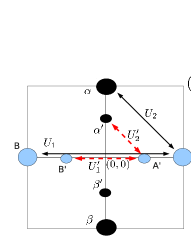
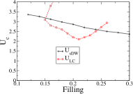
Figure 5: (a) Four new VH points at $(\pm\bar{k},0)$ ($A^{\prime}$ and $B^{\prime}$) and $(0,\pm\bar{k})$ ($\alpha^{\prime}$ and $\beta^{\prime}$) emerge when $t^{\prime\prime}$ (3rd nearest neighbor hopping) is included. (b) The instability boundaries of staggered density wave (solid), liquid crystal (dashed) for $t^{\prime}=-0.4$, $t^{\prime\prime}=0.2$ and $n=0.1-0.3$.

Fig. 5(b) shows the sDW and liquid crystal instabilities for $t=1$, $t^{\prime}=-0.4$, $t^{\prime\prime}=0.2$. For fillings $0.15<n<0.24$, $U_{c}^{LC}<U_{c}^{sDW}$ so the liquid crystal phase will be realized as the dipolar interaction is increased. We have checked that $U_{c}^{LC}$ reaches minimum when the Fermi surface crosses the new set of VH points. Similarly for $t=1$, $t^{\prime}=-0.4$, $t^{\prime\prime}=0.15$, we find the liquid crystal is the leading instability for fillings $0.167<n<0.24$.

Fig. 6 shows the liquid crystal order parameter as a function of $U$ and the representative Fermi surfaces at different $U$ values, for $t=1$, $t^{\prime}=-0.4$, $t^{\prime\prime}=0.2$ at $n=0.2$. At small $U$, the isotropic (normal) phase contains five particle-pockets centered at $(0,0)$, $(\pm\pi,0)$, and $(0,\pm\pi)$. The topology of Fermi surface within the liquid crystal phase changes for $U$ around 2.5. Finally, for $U>6$, the isotropic phase reappears with a single Fermi surface centered at $(0,0)$. This transition is of first order.

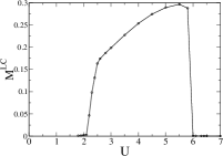
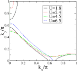
Figure 6: (a) The liquid crystal order parameter as a function of $U$ for $t=1$, $t^{\prime}=-0.4$, $t^{\prime\prime}=0.2$ at $n=0.2$. (b) The Fermi surfaces in the first quadrant of the Brillouin zone for $U=1.8$ (isotropic), 2.4 and 4.5 (liquid crystal), and 6.5 (isotropic).

These features can be understood by a careful analysis of the renormalization of the dispersion by the dipolar interaction within the Hartree-Fock mean field theory of Lin et al. (2010). Especially, the energy landscape evolves differently near the two sets of VH points as $U$ is increased, leading to the nontrivial Fermi surface evolution in Fig. 6(b).

In conclusion, liquid crystal phases can occur in two dimensional dipolar systems. Lattice systems with a band structure containing two sets of VH points are particularly promising to develop the liquid crystal instability. The physical mechanism is the same as outlined in Ref. Lin et al. (2010). While the phase boundary presented in Ref. Lin et al. (2010) was wrong, the discussions on the compressibility and zero sound remain valid. We thank Jim Freericks for drawing our attention to the error in Ref. Lin et al. (2010).

References

- Wigner (1934) E. Wigner, Phys. Rev 46, 1002 (1934).
- Fradkin et al. (2007) E. Fradkin, S. A. Kivelson, and V. Oganesyan, Science 315, 196 (2007).
- Chaikin and Lubensky (1995) P. M. Chaikin and T. C. Lubensky, Principles of Condensed Matter Physics (Cambridge University Press, 1995).
- Kivelson et al. (1998) S. A. Kivelson, E. Fradkin, and V. J. Emery, Nature 393, 550 (1998).
- Yamase and Kohno (2000a) H. Yamase and H. Kohno, J. Phys. Soc. Jpn. 69, 2151 (2000a).
- Oganesyan et al. (2001) V. Oganesyan, S. A. Kivelson, and E. Fradkin, Phys. Rev. B 64, 195109 (2001).
- Kee et al. (2003) H. Y. Kee, E. H. Kim, and C. H. Chung, Phys. Rev. B 68, 245109 (2003).
- Khavkine et al. (2004) I. Khavkine, C. H. Chung, V. Oganesyan, and H. Y. Kee, Phys. Rev. B 70, 155110 (2004).
- Quintanilla and Schofield (2006) J. Quintanilla and A. J. Schofield, Phys. Rev. B 74, 115126 (2006).
- Carlson et al. (2000) E. W. Carlson, D. Orgad, S. A. Kivelson, and V. J. Emery, Phys. Rev. B 62, 3422 (2000).
- Biermann et al. (2001) S. Biermann, A. Georges, A. Lichtenstein, and T. Giamarchi, Phys. Rev. Lett. 87, 276405 (2001).
- Ho et al. (2004) A. F. Ho, M. A. Cazalilla, and T. Giamarchi, Phys. Rev. Lett. 92, 130405 (2004).
- Kollath et al. (2008) C. Kollath, J. S. Meyer, and T. Giamarchi, Phys. Rev. Lett. 100, 130403 (2008).
- Tranquada et al. (1995) J. Tranquada, B. J. Sternlieb, J. D. Axe, Y. Nakamura, and S. Uchida, Nature 375, 561 (1995).
- Orenstein and Millis (2000) J. Orenstein and A. J. Millis, Science 288, 468 (2000).
- Yamase and Kohno (2000b) H. Yamase and H. Kohno, J. Phys. Soc. Jpn. 69, 332 (2000b).
- Kivelson et al. (2004) S. A. Kivelson, E. Fradkin, and T. Geballe, Phys. Rev. B 69, 144505 (2004).
- Lilly et al. (1999) M. P. Lilly, K. B. Cooper, J. P. Eisenstein, L. N. Pfeiffer, and K. W. West, Phys. Rev. Lett. 83, 824 (1999).
- Pan et al. (1999) W. Pan, R. R. Du, H. L. Stormer, D. C. Tsui, K. W. B. L. N. Pfeiffer, and K. W. West, Phys. Rev. Lett. 83, 820 (1999).
- Borzi et al. (2007) R. A. Borzi, S. A. Grigera, J. Farrell, R. S. Perry, S. J. S. Lister, S. L. Lee, D. A. Tennant, Y. Maeno, and A. P. Mackenzie, Science 315, 214 (2007).
- Sun et al. (2008) K. Sun, B. M. Fregoso, M. Lawler, , and E. Fradkin, Phys. Rev. B 78, 085124 (2008).
- Lawler et al. (2006) M. J. Lawler, V. Fernandez, D. G. Barci, E. Fradkin, and L. Oxman, Phys. Rev. B 73, 085101 (2006).
- Halboth and Metzner (2000) C. J. Halboth and W. Metzner, Phys. Rev. Lett. 85, 5162 (2000).
- Koulakov et al. (1996) A. A. Koulakov, M. M. Fogler, and B. I. Shklovskii, Phys. Rev. Lett. 76, 499 (1996).
- Fradkin and Kivelson (2009) E. Fradkin and S. A. Kivelson, Phys. Rev. B 59, 8065 (2009).
- Mancini et al. (2004) M. W. Mancini, G. D. Telles, A. R. Caires, V. S. Bagnato, and L. G. Marcassa, Phys. Rev. Lett. 92, 133203 (2004).
- Buchler et al. (2007) H. P. Buchler, E. Demler, M. Lukin, A. Micheli, N. Prokof’ev, G. Pupillo, and P. Zoller, Phys. Rev. Lett. 98, 060404 (2007).
- Micheli et al. (2007) A. Micheli, G. Pupillo, H. P. Buchler, and P. Zoller, Phys. Rev. A 76, 043604 (2007).
- Sawyer et al. (2007) B. C. Sawyer, B. L. Lev, E. R. Hudson, B. K. Stuhl, M. Lara, J. L. Bohn, , and J. Ye, Phys. Rev. Lett. 98, 253002 (2007).
- Ni et al. (2008) K. K. Ni, S. Ospelkaus, M. H. G. de Miranda, A. Pe’er, B. Neyenhuis, J. J. Zirbel, S. Kotochigova, P. S. Julienne, D. S. Jin, and J. Ye, Science 322, 231 (2008).
- Miyakawa et al. (2008) T. Miyakawa, T. Sogo, and H. Pu, Phys. Rev. A 77, 061603 (2008).
- Fregoso et al. (2009) B. M. Fregoso, K. Sun, E. Fradkin, and B. L. Lev (2009), eprint arXiv/0902.0739.
- Chan et al. (2009) K. T. Chan, C. Wu, W. C. Lee, and S. D. Sarma (2009), eprint arXiv/0906.4403.
- Fregoso and Fradkin (2009) B. M. Fregoso and E. Fradkin (2009), eprint arXiv/0907.1345.
- Baranov et al. (2004) M. A. Baranov, L. Dobrek, and M. Lewenstein, Phys. Rev. Lett. 92, 250403 (2004).
- Bruun and Taylor (2008) G. M. Bruun and E. Taylor, Phys. Rev. Lett. 101, 245301 (2008).
- Zhao et al. (2009) C. Zhao, L. Jiang, X. Liu, W. M. Liu, X. Zou, and H. Pu (2009), eprint arXiv/0910.4775.
- Quintanilla et al. (2009) J. Quintanilla, S. T. Carr, and J. J. Betouras, Phys. Rev. A 79, 031601 (2009).
- Yamase et al. (2005) H. Yamase, V. Oganesyan, and W. Metzner, Phys. Rev. B 72, 035114 (2005).
- Hankevych et al. (2002) V. Hankevych, I. Grote, and F. Wegner, Phys. Rev. B 66, 094516 (2002).
- Nayak (2000) C. Nayak, Phys. Rev. B 62, 4880 (2000).
- Pomeranchuk (1958) I. I. Pomeranchuk, Sov. Phys. JETP 35, 524 (1958).
- Abrikosov (1988) A. A. Abrikosov, Fundamentals of the Theory of Metals (Northa Holland, Amsterdam, 1988).
- (44) Strictly speaking the -density wave is a mean field solution to the extended Hubbard model in the sense that one cannot obtain the value of order parameter from a set of self-consistency equations. However one could use the variational principle to argue that the -density wave has lower energy than the isotropic state. To estimate the critical of -density wave, we first decompose the interaction into , identifying the coefficient common to those in with . We then approximate the interaction as where -density wave is naturally a mean field solution. Note that by doing so, the so called extended -density wave () has the same critical as that of -density wave.
- Yamase (2007) H. Yamase, Phys. Rev. B 76, 155117 (2007).
- Nozires and Pines (1999) P. Nozires and D. Pines, The Theory of Quantum Liquids (Perseus Books, USA, 1999).
- Lamas et al. (2008) C. A. Lamas, D. C. Cabra, and N. Grandi, Phys. Rev. B 78, 115104 (2008).
- Nilsson and Neto (2005) J. Nilsson and A. H. C. Neto, Phys. Rev. B 72, 195104 (2005).
- Wolfle and Rosch (2007) P. Wolfle and A. Rosch, J. Low Temp. Phys. 147, 165 (2007).
- Jordens et al. (2008) R. Jordens, N. Strohmaier, K. Gunter, H. Moritz, and T. Esslinger, Nature 455, 204 (2008).
- Hofstetter et al. (2002) W. Hofstetter, J. I. Cirac, P. Zoller, E. Demler, and M. D. Lukin, Phys. Rev. Lett. 89, 220407 (2002).
- Lin et al. (2010) C. Lin, E. Zhao, and W. V. Liu, Phys. Rev. B 81, 045115 (2010).