Digging into NGC 6334 I(N): Multiwavelength Imaging of a Massive Protostellar Cluster

Abstract

We present a high-resolution, multi-wavelength study of the massive protostellar cluster NGC 6334 I(N) that combines new spectral line data from the Submillimeter Array (SMA) and VLA with a reanalysis of archival VLA continuum data, 2MASS and Spitzer images. As shown previously, the brightest 1.3 mm source SMA1 contains substructure at subarcsecond resolution, and we report the first detection of SMA1b at 3.6 cm along with a new spatial component at 7 mm (SMA1d). We find SMA1 (aggregate of sources a, b, c, and d) and SMA4 to be comprised of free-free and dust components, while SMA6 shows only dust emission. Our $1\farcs 5$ resolution 1.3 mm molecular line images reveal substantial hot-core line emission toward SMA1 and to a lesser degree SMA2. We find CH₃OH rotation temperatures of $165\pm 9$ K and $145\pm 12$ K for SMA1 and SMA2, respectively. We estimate a diameter of 1400 AU for the SMA1 hot core emission, encompassing both SMA1b and SMA1d, and speculate that these sources comprise a $\gtrsim 800$ AU separation binary that may explain the previously-suggested precession of the outflow emanating from the SMA1 region. Compact line emission from SMA4 is weak, and none is seen toward SMA6. The LSR velocities of SMA1, SMA2, and SMA4 all differ by 1-2 km s^-1. Outflow activity from SMA1, SMA2, SMA4, and SMA6 is observed in several molecules including SiO(5–4) and IRAC $4.5~{}\mu$m emission; 24 $\mu$m emission from SMA4 is also detected. Eleven water maser groups are detected, eight of which coincide with SMA1, SMA2, SMA4, and SMA6, while two others are associated with the Sandell et al. (2000) source SM2. We also detect a total of 83 Class I CH₃OH 44 GHz maser spots which likely result from the combined activity of many outflows. Our observations paint the portrait of multiple young hot cores in a protocluster prior to the stage where its members become visible in the near-infrared.

1. INTRODUCTION

The formation process of massive stars is an important but poorly-understood phenomenon. Because most regions that are forming massive stars lie at distances of several kiloparsecs, and most massive stars form in clusters, the identification of high mass protostars requires both good sensitivity and high angular resolution to resolve the continuum and line emission within young protoclusters. The advent of (sub)millimeter interferometers allows the study of deeply-embedded thermal gas emission at arcsecond angular resolution, a realm that has historically been accessible only via maser and cm $\lambda$ continuum emission. Research that combines observations of dust, thermal gas and maser gas offers a more complete picture of the star formation process, as these phenomena potentially trace objects at different evolutionary stages.

NGC 6334 is a luminous ($>10^{6}$ L_☉) and relatively nearby (1.7 kpc; Neckel, 1978) region of massive star formation containing sites at various stages of evolution (Straw & Hyland, 1989). Matthews et al. (2008) have recently completed a comprehensive single dish study of the submillimeter dust properties of the whole complex with $\sim 14\arcsec$ resolution and find a total dust mass of $\sim 1.7\times 10^{4}$ M_⊙. Recent work by Persi & Tapia (2008) suggests that the distance to NGC 6334 may be as close as 1.6 kpc, though we adopt 1.7 kpc for ease of comparison with earlier work. The dust core “I(N)” was first detected at 1 mm by Cheung et al. (1978) and later at $400~{}\mu$m by Gezari (1982) toward the northern end of the complex.

In the past decade, direct evidence of protostars in the I(N) region were found in the form of Class I and II methanol masers (Kogan & Slysh, 1998; Walsh et al., 1998) and a faint 3.6 cm source (Carral et al., 2002). In a previous paper, we presented the first millimeter interferometric observations of I(N) with $\sim 1\farcs 5$ resolution which revealed a cluster of compact dust continuum cores likely to be a protocluster (Hunter et al., 2006, see also Figure 1). Subsequent subarcsecond resolution 7 mm continuum observations by Rodríguez et al. (2007) resolved the principal source SMA1 into several components, and detected possible counterparts to SMA4 and SMA6 (also see Carral et al., 2002). Our recent observations of the ammonia inversion transitions up to (6,6) demonstrated the presence of compact clumps of hot thermal gas within this protocluster (Beuther et al., 2007). Although water masers are excellent tracers of high mass star formation, previous observations of this region have been limited to single dish data (Moran & Rodriguez, 1980). Likewise, most of the millimeter line studies of this region have been performed with single-dish telescopes. For example, Pirogov et al. (2003) imaged the N₂H⁺ (1–0) line with a beamsize of 40″ and found significantly stronger emission toward I(N) than toward the more luminous massive protocluster (source I) that lies $\sim 1\arcmin$ south of I(N). In addition, the SiO (2–1) and (5–4) transitions show strong wing emission from $-50$ to +40 km s^-1 when observed with beamsizes of $58^{\prime\prime}$ and $23^{\prime\prime}$, respectively (Megeath & Tieftrunk, 1999).

Recently, we reported 3 mm interferometric imaging of I(N), which revealed compact CH₃CN (5–4) emission toward SMA1 along with a bipolar outflow seen in HCN(1–0) (Beuther et al., 2008). In this paper, we present the details of our 1.3 mm Submillimeter Array (SMA) spectral line dataset, along with new NRAO Very Large Array (VLA) H₂O maser and 44 GHz Class I CH₃OH maser data. We have also re-analyzed archival VLA continuum data from 3.6 cm to 7 mm, 2MASS near-IR and Spitzer mid-IR IRAC and MIPS images. Together these data confirm the identification of NGC 6334 I(N) as an actively forming massive protostellar cluster.

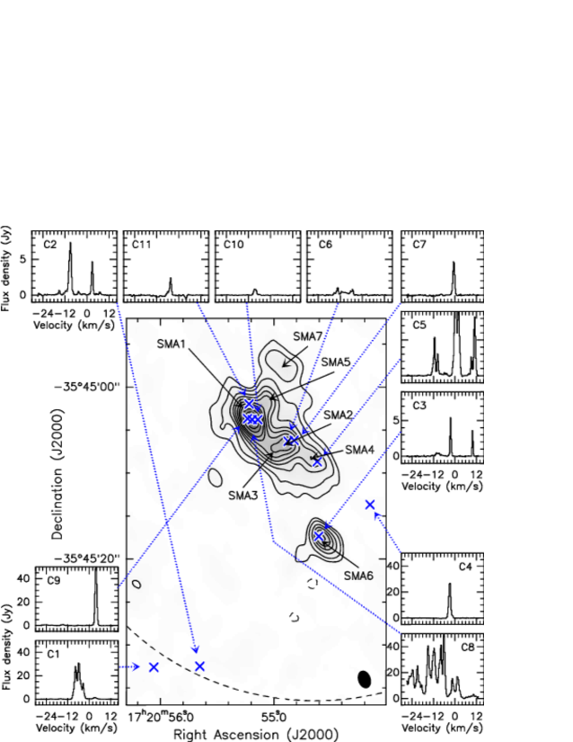
Figure 1.— Composite image showing the naturally weighted SMA 1.3 mm continuum emission from I(N) with surrounding insets showing the VLA H₂O (22.235 GHz) maser spectra. The 1.3 mm continuum image has a resolution of $2\farcs 2\times 1\farcs 3$ (P.A.=+15°) and the contour levels are 30 ($3.5\sigma$), 60, 120, 180, 240, 320, 400, 640, 800, 960 mJy beam^-1. The blue crosses show the intensity weighted centroid positions of the water maser groups listed in Table Digging into NGC 6334 I(N): Multiwavelength Imaging of a Massive Protostellar Cluster (derived from Table 3). The water maser spectra show the average emission from each group. The dashed arc indicates the SMA primary beam, and the dashed arc indicates the VLA primary beam at 22 GHz. The 1.3 mm image has not been corrected for primary beam attenuation.

2. OBSERVATIONS

2.1. Submillimeter Array (SMA)

Our SMA observations were made with six antennas – in May 2004 in the compact configuration, and in May 2005 in the extended configuration. In both tracks, two pointings were observed: source I at 17^h20^m53.44^s, $-35\arcdeg 47\arcmin 02.2\arcsec$ and source I(N) at 17^h20^m54.63^s, $-35\arcdeg 45\arcmin 08.5\arcsec$ (J2000). Only the data for source I(N) are presented in this paper. The SMA receivers are double sideband SIS mixers with 2 GHz bandwidth (Blundell et al., 1998). The local oscillator was tuned to provide 216.6-218.6 GHz in LSB and 226.6-228.6 GHz in USB, yielding a FWHP primary beam size of $\sim 55\arcsec$. The correlator was configured for 3072 channels per sideband with a uniform spectral resolution of 0.8125 MHz. The correlator sideband separation was about 18 dB at the time of these observations. Typical system temperatures were 200 K. The projected baseline lengths ranged from 10 to 180 m. A continuum image produced from these data was presented in Hunter et al. (2006), however in order to correct for a half-channel error in SMA velocity labeling discovered in November 2007, the data have been completely re-reduced.

The gain calibrators were the quasars NRAO 530 ($23^{o}$ distant) and J1924$-$292 ($27^{o}$ distant). Bandpass calibration was performed with observations of Uranus (2004 data) and 3C279 (2005 data). Flux calibration is based on observations of Jovian satellites and regular SMA monitoring of the quasar flux densities. The data were calibrated in Miriad, then exported to AIPS for imaging; the two sidebands were reduced independently. The AIPS task UVLSF was used to separate the line and continuum emission. Self-calibration was derived from the continuum, and solutions were transferred to the spectral line data. After self-calibration, the continuum data from both sidebands were combined and imaged with both natural and uniform weighting in order to achieve the best surface brightness sensitivity (the former) and best angular resolution (the latter). The naturally weighted image has an angular resolution of $2\farcs 2\times 1\farcs 3$ at P.A. $+15^{\circ}$ and the uniformly weighted image has an angular resolution of $1\farcs 8\times 0\farcs 9$ at P.A. $+8^{\circ}$. The rms noise levels are 8.4 and 6.4 mJy beam^-1 for the natural and uniform weighted images, respectively. The peak signal-to-noise of the naturally weighted continuum image has increased to 126 compared to 114 for the image presented in Hunter et al. (2006). The spectral line data were resampled to a spectral resolution of 1.1 km s^-1 and imaged with natural weighting; the rms noise per channel is 180 mJy beam^-1. The absolute position uncertainty of these data is estimated to be 0$\farcs$3.

2.2. Very Large Array (VLA)

2.2.1 Water Maser Observations

The 1.3 cm (22.235 GHz) H₂O maser data were taken with the VLA on 2006 July 03 (project AH915) with online Hanning smoothing and one polarization (RR). The full bandwidth of the data is 3.125 MHz (40 km s^-1 usable) and the channel separation and resolution is 24.4 kHz (0.33 km s^-1). The absolute flux scale was set assuming a 22.235 GHz flux density of 2.54 Jy for 3C286. Fast-switching was employed using J1717-337 and a cycle time of 2 minutes. The calibrator J1924-292 was used for bandpass calibration. The pointing model was updated once per hour during the observation. After flagging periods of poor phase coherence (due to weather), the on-source time is approximately 60 minutes. The FWHM primary beam of these data is $120^{\prime\prime}$ and the synthesized beam is $0\farcs 79\times 0\farcs 25$ at P.A.=+7°.

It was necessary to remove the remarkably strong masers detected toward NGC 6334 I in the sidelobes ($112\arcsec$ from the phase center of I(N)) in order to achieve high dynamic range on the target masers in source I(N); source I masers were detected with peak intensities (uncorrected for primary beam attenuation) as high as 112 Jy beam^-1 despite their location near the first null. The removal was accomplished by self-calibrating the data on the strongest source I channel, applying this calibration to the full line dataset, imaging both fields, subtracting the clean components from source I (only) in the $u-v$ plane (UVSUB), inverting the calibration (CLINV), re-self-calibrating on the strongest I(N) maser channel, applying these new corrections and making the final I(N) line cube (this process is often called “peeling”). This procedure improved the dynamic range in the I(N) channels at the same velocities as the strong source I masers by a factor of $\sim 3$. The rms noise in a single channel is 6 mJy beam^-1. The absolute position uncertainty is approximately $0\farcs 01$. Flux density measurements were made on an image corrected for primary beam attenuation.

2.2.2 44 GHz Methanol Maser Observations

The 7 mm (44.06941 GHz) Class I CH₃OH ($7_{0,7}-6_{1,6}$) A⁺ maser transition was observed on 2008 February 18 with the VLA in CnB-configuration (project code AC904). Correlator mode 2AB was used with a velocity channel width of 0.17 km s^-1. NGC6334I(N) was observed for 7.5 minutes (on-source) as a check source for a larger survey of massive protostellar candidates (Cyganowski et al., 2009). The gain, bandpass, and flux calibrators were J1717-337, J2253+161, and 3C286, respectively. Fast switching was employed with a cycle time of 2 minutes. The absolute positions are expected to be better than $0\farcs 2$. The synthesized beam is $1\farcs{30}\times 0\farcs{40}$ at P.A. = $-44^{\circ}$, and the velocity resolution is 0.33 km s^-1 after Hanning smoothing. Due to the snapshot nature of these data, and consequent poor $u-v$ coverage, the noise is dynamic range limited in channels with strong maser emission. Channels with relatively weak maser emission have rms noise levels of $\sim 100$ mJy beam^-1, while it is up to $5\times$ poorer in channels with strong maser emission (i.e. peak $>50$ Jy).

2.2.3 Archival 7 mm, 1.3 cm, and 3.6 cm Continuum Observations

We have re-reduced the archival VLA 7 mm and 1.3 cm continuum observations originally presented by Rodríguez et al. (2007, project codes AZ159 and AZ152, further details of these observations can be found in that paper). We achieved a significantly better rms noise in the 7 mm image (210 $\mu$Jy beam^-1) than those authors report (320 $\mu$Jy beam^-1). This improvement is likely due to the fact that we simultaneously imaged a field toward source I which contains a strong ultracompact H ii region ($2\arcmin$ south of I(N), see for example Hunter et al., 2006); images made without cleaning this H ii region show significant sidelobes at the location of I(N). We also used the AIPS task VLANT to retrieve and apply post-observation antenna position corrections to the data, and used a model for the brightness distribution of the flux calibrator 3C286. The flux densities derived for the phase calibrator (J1720-355) are within $2\%$ of those reported by Rodríguez et al. (2007). The angular resolution of the 7 mm data is $0\farcs 65\times 0\farcs 44$, P.A.=$+25\arcdeg$. The 1.3 cm data were reduced in a similar manner and the rms noise is 64 $\mu$Jy beam^-1, similar to that obtained by Rodríguez et al. (2007); the angular resolution is $0\farcs 38\times 0\farcs 27$, P.A.=$+19\arcdeg$. The 1.3 cm and 7 mm data show remarkable position agreement given that they were observed on different days – a testament to the accuracy of the VLA when reference pointing and fast switching are employed. We estimate that the absolute position accuracies for these two datasets are better than $0\farcs 05$.

We have also re-reduced the archival VLA 3.6 cm continuum observations originally presented by Carral et al. (2002, project code AM495, further details of the observing parameters can be found in that paper). The pointing center for these data is located $1.5\arcmin$ south of source I(N) (the 3.6 cm FWHP is $5\farcm 4$). These data were re-reduced as described above for the 7 mm and 1.3 cm data. In particular, a model for the brightness distribution of the flux calibrator (3C286) was employed – a method not available at the time of the original Carral et al. (2002) reduction. The average flux densities (between the two IFs) derived for the two phase calibrators, J1733-130 and J1751-253 are $6.67\pm 0.03$ and $0.267\pm 0.001$, respectively. In contrast Carral et al. (2002) obtained $7.6\pm 0.2$ for J1733-130, $14\%$ higher than our more accurate result (a flux density for J1751-253 was not reported by these authors). After self-calibration, the final image was made with baselines longer than 100k$\lambda$ to minimize artifacts from the nearby (within $2\arcmin$) extended H ii regions ”I” and ”E”, which fall within the VLA 3.6 cm FWHP primary beam. The resolution of the final 3.6 cm image of the I(N) region is $0\farcs 51\times 0\farcs 20$, P.A.=$-1\arcdeg$ and the rms noise is 41 $\mu$Jy beam^-1 after primary beam correction (Carral et al., 2002, report an rms noise of 60 $\mu$Jy beam^-1 but it is unclear whether they applied primary beam correction). The 3.6 cm data did not employ reference pointing or fast switching, and we estimate an absolute position accuracy for these data of $0\farcs 3$. We note that there is a consistent $0\farcs 2$ offset (to the SE) between the 3.6 cm data and the 1.3 cm and 7 mm data; we have not shifted the images to match.

2.3. Archival Australia Telescope Compact Array (ATCA) 3.4 mm Observations

We have re-imaged the 3.4 mm ATCA continuum data reported by Beuther et al. (2008). The rms noise is 3.3 mJy beam^-1 (after primary beam correction) and the resolution is $2\farcs 3\times 1\farcs 8$, P.A.=$83\arcdeg$. Due to the small primary beam of the ATCA at this wavelength (FWHP $33\arcsec$), primary beam correction for this image is critical. This accounts for the apparent increase in rms noise compared to that reported by Beuther et al. (2008, 2.6 mJy beam^-1; our rms noise is 2.2 mJy beam^-1 before primary beam correction); the peak signal-to-noise has increased by a factor of 1.3. We estimate an absolute position accuracy for these data of $0\farcs 3$.

2.4. Archival Infrared Data

For near-infrared photometry, we analyzed archival 2MASS survey images (Skrutskie et al., 2006). We have also examined all of the Spitzer archival data for the I(N) region. Of the available IRAC data (Fazio et al., 2004), the data obtained in project 46 on 2004, August 2 by PI Fazio are by far the deepest (666 s). In this paper we use the PBCD images produced by pipeline version 14.0 Hunter et al. (a different version of these data were also presented in 2006). Since saturation in the I(N) region was not an issue, only the long integration (10.4 s) data are used. Unfortunately, of the available MIPS data, only the 24 $\mu$m data are usable – the 70 and 160 $\mu$m data show tremendous striping and other artifacts. In this paper we utilize the 24 $\mu$m data from the MIPSGAL Legacy survey (Carey et al., 2009).

We performed aperture photometry on all infrared images by defining irregular polygonal shapes (the “source” shape) surrounding each extended knot of emission (presumed to be shock fronts from one or more outflows, not point sources). A background is taken as the mode of pixel values in an scaled annulus, between 1.5 and 2 times radially expanded from the centroid of the source shape. These polygons are translated to each infrared image by their locations on the sky, so sample the identical regions even though the images have different pixel sizes and world coordinate systems. Fluxes were converted to Jy using the photometric information for each observatory.

2.5. Caltech Submillimeter Observatory (CSO)

Our CSO observations were obtained on 13 April 1993 using the facility 345 GHz SIS receiver with lead junctions (Ellison et al., 1989) and a 500 MHz AOS backend. Several on-the-fly maps of the CO 3–2 line were obtained on a 10″ grid, providing near-Nyquist sampling of the 20″ beam of the telescope at this frequency. At the end of each row, a designated off position (17^h24^m56.06^s, $-36\arcdeg 21\arcmin 40.1\arcsec$ J2000) relatively free of CO emission was observed to provide the spectral baseline. After combining the maps, the total area covered was $4\arcmin\times 4\arcmin$ ($25\times 25$ grid), with 30 seconds of on-source integration per point in the central portion containing source I and I(N), and 15 seconds per point on the periphery. The DSB receiver temperature was measured to be 320 K using the y-factor method, and the typical SSB system temperature was 1800 K at an elevation of 30°. The spectra have been corrected to the main beam brightness temperature scale using an efficiency of 68% as measured on Jupiter on the same night.

3. RESULTS

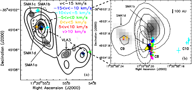
Figure 2.— Zoomed multiwavelength images of I(N). (a) Zoom shows the SMA1, SMA2, and SMA3 regions with thick contours showing the uniformly weighted SMA 1.3 mm continuum image with contour levels of 170, 250, 330, 490, and 650 mJy beam^-1. Thin contours and greyscale show the VLA 7 mm continuum emission (contour levels are -0.6, 0.6, 0.8, 1.0, 1.2 mJy beam^-1). The water maser positions are shown as colored crosses with a corresponding color coded velocity legend; note that the color scale was set using an assumed $-3$ km s^-1 systemic velocity for SMA1. (b) Zoom of the SMA1 region at 3.6 cm (dashed contours), 1.3 cm (greyscale),and 7 mm (solid contours). The 3.6 cm contour levels are 0.12, 0.20, 0.28, and 0.36 mJy beam^-1, and the 7 mm contour levels are same as in (a). The water maser positions are also indicated with the same velocity color coding as (a). The position of the 44 GHz CH₃OH maser is indicated by the yellow ellipse and it has a velocity of $-0.9$ km s^-1. For both types of maser symbol size indicates position uncertainty.

Our multiwavelength images reveal several sites of star formation activity within the I(N) region. In the following sections, we describe the variety of observed phenomena. In the following sections linear offsets are given with the $\gtrsim$ symbol to indicate that the measured values are lower limits since only the projected separation is available (a distance of 1.7 kpc is assumed).

3.1. SMA 1.3 mm Continuum

The naturally weighted 1.3 mm SMA continuum image of I(N) is presented in Figure 1 (center). This image is qualitatively similar to that presented in Hunter et al. (2006), but the calibration has been refined for improved signal-to-noise. These data resolve the presence of at least seven 1.3 mm “cores” in I(N). As pointed out in Hunter et al. (2006), this region has the hallmarks of a “protocluster”, i.e. a region that will form a cluster of intermediate to massive stars. The integrated flux density within the $3\sigma$ contour (30 mJy beam^-1, see Fig. 1) of the naturally weighted 1.3 mm continuum image is $7.4\pm 0.8$ Jy (this is 1.6 times higher than reported in Hunter et al., 2006); this estimate includes both statistical and $10\%$ calibration uncertainties. Sandell (2000) find a 1.3 mm single dish flux density of $14.2\pm 0.2$ Jy, implying that we have recovered about $50\%$ of the total flux with the SMA.

We have used the uniformly weighted image corrected for primary beam attenuation to fit the seven peaks identified in Figure 1 with a single 2-D Gaussian (using JMFIT in AIPS). The fitted positions and flux densities of the 1.3 mm cores are listed in Table 1. SMA1, SMA4, and SMA6 in particular, are not well-fit by a single Gaussian component, and instead appear to have a compact (unresolved, FWHM $<1\arcsec$) region of emission, embedded in a more extended though still compact (FWHM $<3\arcsec$) region. However, attempts to uniquely disentangle these two (or more) components with the current resolution and sensitivity were not successful. The JMFIT sizes listed in Table 1 are representative of the more extended (though still compact on the scale of the I(N) protocluster) component, and the integrated intensities and other quantities calculated from it ($T_{b}$ and mass) are likely to be underestimates. These sizes while quite significant from a signal-to-noise perspective should be viewed as upper limits.

3.2. ATCA 3.4 mm Continuum

As first discussed by Beuther et al. (2008), the 3.4 mm continuum emission toward I(N) (not shown) is qualitatively similar to that at 1.3 mm. With our new imaging of the original Beuther et al. (2008) data, we have been able to increase the signal-to-noise and reliably detect SMA4 at this wavelength. The fitted (JMFIT) parameters of the compact 3 mm continuum emission are given in Table 1.

3.3. VLA Water Masers and Continuum Emission

The association of water masers with molecular outflows make them a good tracer of protostellar activity (Tofani et al., 1995; Hofner & Churchwell, 1996). We find strong 22 GHz H₂O maser emission toward 11 distinct regions in NGC 6334 I(N), listed in Table Digging into NGC 6334 I(N): Multiwavelength Imaging of a Massive Protostellar Cluster in order of increasing declination. Masers that lie in close proximity to each other ($<1\arcsec$) are collectively called by “group” names C1, C2…C11. The intensity weighted positions of these groups are listed in Table Digging into NGC 6334 I(N): Multiwavelength Imaging of a Massive Protostellar Cluster and are plotted on the 1.3 mm continuum image in Figure 1, along with average spectra for each group (the position of each distinct H₂O maser and its velocity are presented in Table 3, available in its entirety online). Eight of the groups lie within 2″ of the 1.3 mm sources SMA1, SMA2, SMA4, and SMA6, whose positions are listed in Table 1. Two of the maser groups (C1 and C2) lie near the SW edge of the SMA primary beam. These masers are coincident with the single-dish millimeter continuum source SM2, identified in JCMT submillimeter continuum images by Sandell (2000). Maser group C4 appears in a region with no compact millimeter continuum emission at the present sensitivity. Instead it lies at the southern edge of the $4.5~{}\mu$m nebula that extends to the southwest from SMA4 (Hunter et al., 2006, also see §3.6). More detailed phenomenology for the SMA 1.3 mm cores (except SMA5 and SMA7 which are weak and fairly diffuse) are given below.

3.3.1 SMA1, SMA2, and SMA3 Regions

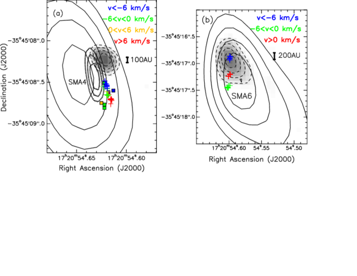
Figure 3.— (a) Zoom of the SMA4 region with the grayscale and dashed contours showing the 1.3 cm continuum emission, dotted contours showing 3.6 cm, and the solid contours showing the uniformly weighted 1.3 mm continuum. The 3.6 cm contours are 0.12, 0.16, and 0.20 mJy beam^-1, the 1.3 cm contour levels are 0.19, 0.25, 0.31, and 0.37 mJy beam^-1, and the 1.3 mm contour levels are 100, 120, 140, and 160 mJy beam^-1. (b) Zoom of the SMA6 region with the greyscale and dashed contours showing 7 mm continuum emission and the solid contours showing the 1.3 mm continuum. The 7 mm contour levels are 0.6, 0.8, 1.0, and 1.2 mJy beam^-1, and the uniformly weighted 1.3 mm contour levels are 100, 140, 180, 220, and 260 mJy beam^-1. The cross symbols show the C5 (a) and C3 (b) water maser positions with S/N ratio $>7$, color-coded by velocity. The filled square symbols in (a) show the location of 6.7 GHz CH₃OH masers from Walsh et al. (1998), with same velocity coding as H₂O masers.

Figure 2a shows a close-up view of the region from SMA1 through SMA3 in both 1.3 and 7 mm continuum. This region also contains H₂O maser groups C6 through C11. Following Rodríguez et al. (2007) we call lower frequency continuum emission that appears to be associated with a particular SMA source by the “SMA name”. If more than one source is associated with a 1.3 mm source, the SMA name is appended by a,b,c etc. Lower frequency continuum emission that is not clearly associated with any particular SMA source is called “VLA” followed by the number of the closest SMA source. From the improvement in the 7 mm image quality over that shown in Rodríguez et al. (2007), several new features are present: (1) The 7 mm source SMA1b is resolved into two distinct sources separated by $\sim 0\farcs 45$ ($\gtrsim 800$ AU, also see Figure 2a), we shall refer to the eastern component as SMA1d; (2) SMA1a is elongated NE/SW and appears to point toward SMA1b; (3) Two new 7 mm features are detected to the north of SMA2 and SMA3, the stronger of the two is closest to SMA3 ($\sim 1\arcsec$ north), and is thus called VLA3, while the other is barely above the $3\sigma$ level and is not discussed further. The flux densities and positions of all of the continuum sources from 1.3 mm to 3.6 cm are provided in Table 1.

Figure 2b further zooms in on the continuum emission from SMA1b and SMA1d and the maser groups C8, C9, and C10. From this figure it is clear that SMA1d is also distinct from SMA1b at 1.3 cm. From our reanalysis of the 3.6 cm data originally reported by Carral et al. (2002) we also detect SMA1b at this frequency. As mentioned in §2.2 there appears to be a systematic $0\farcs 2$ position offset of the 3.6 cm data which if removed would cause it to match the 1.3 cm and 7 mm position for SMA1b. Maser group C8, located $\sim 0\farcs 3$ south of SMA1b, contains the brightest H₂O maser in the whole region and is resolved into a linear north/south structure $\gtrsim 800$ AU in length. The velocity structure of this linear group of masers is broad and complex, although the northern part is mostly blueshifted while the southern part is mostly redshifted with respect to the $\sim-3$ km s^-1 systemic velocity of SMA1 (see §3.5 for discussion of systemic velocities). These characteristics are similar to the brightest H₂O maser component (C6) in the protocluster AFGL 5142 (Hunter et al., 1999) but on a somewhat larger physical scale. A 44 GHz maser with a velocity of $\sim-0.9$ km s^-1 is also coincident with this linear H₂O maser feature.

The redshifted and kinetically narrow H₂O maser group C9 is coincident with SMA1d and contains the second brightest maser feature in I(N). A weak blueshifted group of masers (C10) lies $\gtrsim 1200$ AU southeast of SMA1b. Back on the larger scale of Fig. 2a, group C11 is another blueshifted narrow feature that lies $\gtrsim 1300$ AU northwest of SMA1c. Group C6 is $\gtrsim 400$ AU northwest of SMA2 and is blueshifted with respect to the systemic velocity of SMA2 ($\sim-5$ km s^-1; see §3.5). Group C7 is a narrow but fairly strong component $\gtrsim 1500$ AU northwest of SMA2, and is near the systemic velocity.

3.3.2 SMA4 Region

Looking further south toward SMA4, the spatial/velocity structure of water maser group C5, as well as the 1.3 mm and 1.3 and 3.6 cm continuum emission in this region is shown in Figure 3a. There are three distinct spatial clusters of H₂O masers within the C5 group, corresponding to the three different velocity components. These three clusters of masers are oriented roughly north/south (P.A.=$17\arcdeg$) with blueshifted emission to the north, and redshifted emission to the south. The C5 group lies within $0\farcs 4$ ($\gtrsim 700$ AU) of the 1.3 mm to 3.6 cm continuum emission peaks, just within the combined astronomical uncertainties of the data. The C5 group is also coincident with a cluster of Class II 6.7 GHz CH₃OH masers (Walsh et al., 1998; Caswell, 2009) which have a similar velocity gradient. The 1.3 and 3.6 cm emission has been reported previously by Rodríguez et al. (2007) and Carral et al. (2002), respectively. We report the detection of SMA4 at 7 mm (not shown, see Table 1). As mentioned in §2.2 there appears to be a systematic offset of $0\farcs 2$ of the 3.6 cm data which if removed would cause it to match the 1.3 cm and 7 mm position. It is currently unclear if the maser and 1.3 mm offsets are significant (or simply due to absolute position uncertainties).

3.3.3 SMA6 Region

A zoomed in view of the SMA6 region is shown in Figure 3b. The C3 group of water masers is coincident with SMA6 and also has three distinct velocity clusters (see Fig. 3b). The kinematics of C3 are curious, with the three clusters lying along a roughly north-south line with systemic velocity to the south, then redshifted in the middle, and then blueshifted emission to the north. The 7 mm continuum peak toward SMA6 lies $\gtrsim 700$ AU north of the 1.3 mm peak, coincident with the northern blueshifted cluster of C3 masers. SMA6 is not detected at wavelengths longer than 7 mm. The 1.3 mm morphology of SMA6 is suggestive of unresolved substructure in the north-south direction, and as mentioned in §3.1 is not well fit by a single Gaussian. Interestingly, although the 7 mm data has significantly better spatial resolution than the 1.3 mm data, both images show a similar morphology.

3.4. VLA 44 GHz Methanol masers

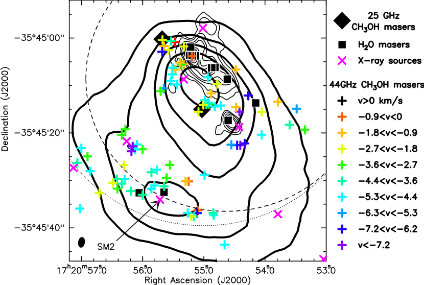
Figure 4.— SMA 1.3 mm continuum contours of I(N) (thin black contours) with thick black contours showing SCUBA 450 $\mu$m emission (G. Sandell, private communication). The 1.3 mm continuum image and contour levels are the same as Fig. 1. The SCUBA 450 $\mu$m resolution is $8\arcsec$ and the contour levels are 60, 80, 100, 120, 160 Jy beam^-1. The tip of the arrow for SM2 is the position reported by Sandell (2000). The colored crosses show the locations of 44 GHz Class I methanol masers from this work. The locations of the water maser groups (also see Fig. 1) are shown by $\blacksquare$ symbols and the 25 GHz CH₃OH masers reported by Beuther et al. (2005) are shown by $\blacklozenge$ symbols. The X-ray sources from Feigelson et al. (2009) are marked by magenta X’s. The dashed arc indicates the SMA primary beam and the dotted arc indicates the VLA 44 GHz primary beam. The 1.3 mm SMA continuum resolution is shown in the lower left.

Strong 44 GHz CH₃OH maser emission from NGC 6334 I(N) was first detected in the single dish survey of Haschick et al. (46″ beam; 1990). Kogan & Slysh (1998) resolved this emission into 23 spots using ten antennas of the VLA, but they were unable to determine accurate absolute positions. Our new observations with the full VLA provide a deeper more accurate view of the maser emission. By examining and comparing the details of the emission in each channel and from channel to channel, we have identified 83 individual maser spots. These are listed in Table 4, available in its entirety online. The values of $v_{\rm peak}$ refer to the center velocity of the channel in which the peak emission occurs. The tabulated positions are the fitted position in the peak channel for each component. The peak brightness temperatures of these masers (see Table 4) lie far above the energy level of this transition (65 K, 43.7 cm^-1), with values as high as $T_{b}=3.6\times 10^{5}$ K with the current spatial resolution. While we have detected far more spots of emission, the spatial and velocity distribution of the Kogan & Slysh (1998) spots are quite consistent with our data if one shifts the Kogan & Slysh (1998) positions by 7.3″ to the south-southwest. At the current level of sensitivity, no thermal emission was detected.

The maser positions are shown as velocity color-coded crosses in Figure 4.3. The peak maser velocities are in the range $-8.49$ to $-0.35$ km s^-1, close to the systemic velocity of the region. Figure 4.3 also shows a 450 $\mu$m JCMT continuum image with $8\arcsec$ resolution from Sandell (2000). The masers are distributed over much of the area of dust emission, as delineated by the lowest $450~{}\mu$m contour. The masers can be divided into two main concentrations: the general area of the compact SMA continuum sources, and the area around the single-dish source SM2 (Sandell, 2000). The former concentration contains a more diverse range of velocities, though no obvious trends in kinematics versus position are seen. It is notable that while these masers are clustered around I(N) 1.3 mm continuum sources, only one is positionally coincident with a compact SMA source (SMA1, see Fig. 2). The latter concentration towards the single dish continuum source SM2 is not associated with any 1.3 mm SMA continuum emission but this region lies outside the half-power point of the SMA data, significantly reducing the sensitivity in this region. Two 25 GHz Class I CH₃OH masers were also detected toward I(N) by Beuther et al. (2005), and both of these are coincident with 44 GHz maser emission and have comparable velocities as shown in Fig. 4.3.

The position of the X-ray sources recently reported for this region (Feigelson et al., 2009) are also shown in Figure 4.3. The median photon energy of many of these X-ray sources is relatively hard (E ¿ 4 keV), suggesting deeply embedded sources. These authors have already noted the possible association of X-ray source 1454 with SMA7, and 1447 with SMA6 (although the latter is less likely given that its median photon energy is only 1 keV). With our new data, we note four additional possible associations: X-ray source 1470 is within $1\farcs 8$ of the water maser component C2; and X-ray sources 1463, 1477 and 1487 each reside within a few arcseconds of a cluster of methanol masers. Source 1463 lies SSE of SMA1, just beyond the lowest millimeter contour. Source 1477 aligns with the shoulder of $450~{}\mu$m emission northeast of SM2, while source 1487 lies just east of the lowest $450~{}\mu$m contour

3.5. SMA 1.3 Millimeter Molecular Line Data

A total of 79 lines from 19 molecular species are detected toward SMA1 (Table 5) along with 14 unidentified features within the 4 GHz of total bandwidth observed by the SMA. The spectra toward the SMA1 1.3 mm continuum peak are shown in Figure 5. The lines were indentified using the CDMS (Müller et al., 2001), JPL (Pickett et al., 1998), and Splatalogue spectral line databases. The large number of organic transitions detected, coupled with modest line brightness temperatures of 30 K suggests that this source harbors a moderate “hot core” (van Dishoeck & Blake, 1998). Many of the stronger lines detected toward SMA1 are also detected toward SMA2, though most are weaker, suggesting that this source also harbors a weak hot core. Other sources observed with similar linear resolution with this SMA setup have yielded both less diverse (S255N, Cyganowski et al., 2007), as well as much richer hot core spectra (NGC6334I, Brogan et al., in prep). The broadband SEST single-dish molecular line survey toward NGC 6334I and I(N) also shows that while source I(N) exhibits significant hot core emission, source I shows a much richer array of molecular line species along with stronger emission (Thorwirth et al., 2003).

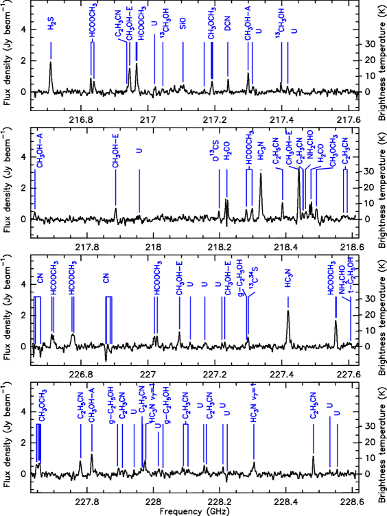
Figure 5.— SMA spectra of the upper and lower sidebands from the 1.3 mm continuum peak of NGC6334I(N)-SMA1. The spectra have been Hanning smoothed.

3.5.1 Extended Molecular Line Emission

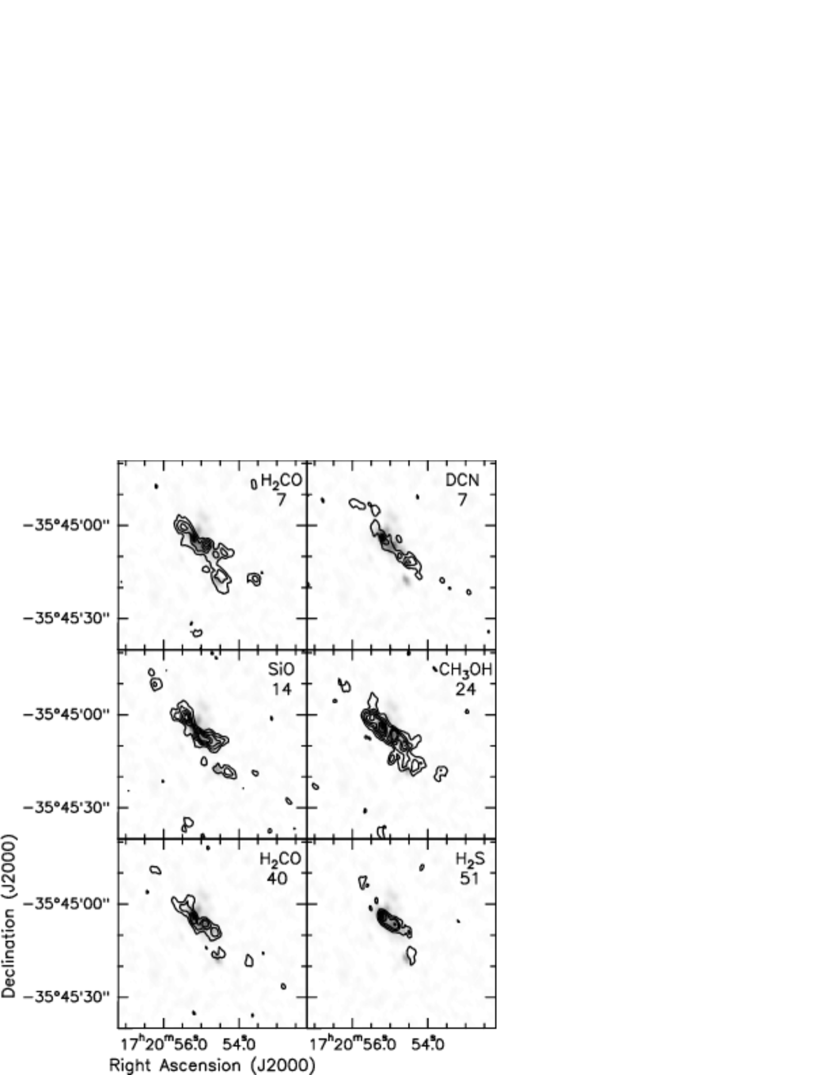
Figure 6.— In each panel, the colorscale is the 1.3 mm continuum and the contours show the integrated intensity of the indicated spectral lines. The dashed circle is the FWHP of the SMA primary beam; these images have not been corrected for primary beam attenuation. The contour levels are H₂CO ($3_{0,3}-2_{0,2}$): 4.35, 7.25, 10.15, 13.05 Jy km s^-1; DCN: 1.77, 2.95, 4.13 Jy km s^-1; SiO: 6, 10, 14, 18, 22 Jy km s^-1; CH₃OH-E ($4_{+2,2}-3_{+1,2}$): 4.8, 8, 11.2, 14.4, 17.6 Jy km s^-1; H₂CO ($3_{2,2}-2_{2,1}$): 3.24, 5.4, 7.56 Jy km s^-1; H₂S: 2.55, 4.25, 5.95, 9.35 Jy km s^-1. The number below each molecular name is the $E_{\rm lower}$ of the transition in units of cm^-1.

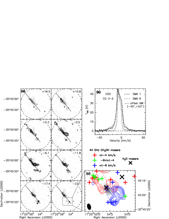
Figure 7.— (a) Channel maps of SiO 5–4. In each panel, the greyscale is the 1.3 mm continuum emission and the contours are SiO emission (levels = 0.29, 0.48, 0.67, 0.86, 1.05 Jy). The outflow axis is drawn at position angle $+39\arcdeg$. The dashed circle is the SMA primary beam. (b) CSO CO (3–2) spectra taken near SMA1, SMA6 and a position offset $-40\arcsec,+53\arcsec$ to the northwest (away from any obvious outflow emission). The SMA1 spectrum was taken 2.9″ from SMA1, and the SMA6 spectrum is the average of the three spectra taken closest to SMA6 (5″, 7″, and 8″ away). (c) Close up of SiO (5–4) outflow around SMA6. The contours show SiO (5–4) integrated emission, red contours show integrated intensity from +17 to -6 km s^-1 and blue contours show integrated intensity from from -8 to -31 km s^-1. The CH₃OH and H₂O maser positions are also shown. The solid black ellipse is the SMA synthesized beam.

Many of the lines from low excitation states ($E_{l}<$ 70  cm^-1) show emission extending to the NE and SW of the SMA continuum emission (see Figure 6). This emission is clearly tracing one or more outflows emanating from the protocluster. Interpretation of the extended emission is complicated by the fact that the SMA data are not sensitive to smooth emission on sizescales $\gtrsim 20\arcsec$ (due to spatial filtering by the interferomter). Generally, the emission to the northeast is red-shifted, while that to the southwest is blueshifted, but the kinematics become very confused in the southern part of I(N) with both red and blueshifted emission present. SiO in particular shows a striking bipolar appearance centered on SMA1. Channel maps of SiO (Figure 7a) reveal the complex velocity field of the extended emission. A lobe of molecular material also extends westward from SMA4 at low, but blueshifted velocities in SiO and several other species shown in Fig. 6 (H₂CO, CH₃OH, and H₂S for example).

A more compact SiO velocity gradient also appears to be centered on SMA6. CSO CO(3–2) spectra with 20″ resolution show that the broad line wings toward SMA6 are of similar magnitude to those seen toward SMA1 (see Fig. 7b), suggesting both objects harbor outflows. The integrated red and blue-shifted emission around SMA6 is shown in detail in Figure 7c, and is more or less centered on the CN and H₂CO ($E_{l}=7$ cm^-1) absorption velocity of $\sim-4$ km s^-1 (see §3.5.2). This figure also shows that the sense of the SiO gradient is reflected in the position and velocity of the 44 GHz methanol masers surrounding SMA6. However, on smaller scales the C3 group of water masers is oriented in a more north-south direction (Fig. 3b). It is unclear how the curious kinematics of the C3 water masers (from south to north: systemic, then red, then blueshifted features) fits in with the compact NE-SW outflow.

3.5.2 Compact Molecular Line Emission and Absorption

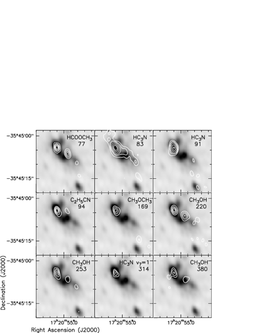
Figure 8.— In each panel, the greyscale is the 1.3 mm continuum and the contours are drawn from moment-zero images of spectral lines. The contour levels are: HCOOCH₃: 2.1, 4.2, 6.3, 8.4, 10.5 Jy km s^-1; HC₃N: 2.55, 4.25, 5.95, 9.35, 14.45, 19.55 Jy km s^-1; C₂H₅CN: 1.8, 3.0, 4.2, 5.4 Jy km s^-1; CH₃OCH₃: 1.35, 2.25, 3.15 Jy km s^-1; CH₃OH(220): 1.89, 3.78, 5.67, 7.56 Jy km s^-1; 2.31, 3.85, 5.39, 6.93 Jy km s^-1; HC₃N(v₇=1): 1.5, 2.5, 3.5 Jy km s^-1; CH₃OH(380): 2.1, 3.5, 4.9 Jy km s^-1. The numbers below each molecular name is the $E_{\rm lower}$ of the transition in units of cm^-1.

As seen in Figure 8, emission from the higher excitation lines ($E_{l}>$ 70 cm^-1) is concentrated toward SMA1. In several species, a secondary peak of emission appears toward SMA2. Indeed, the SMA2 peak in methyl formate and the lower lying transitions of methanol is almost equal to that of SMA1. A few vibrational states of CH₃OH and HC₃N are detected exclusively toward SMA1, suggesting that it is warmer and/or denser than SMA2. Several species also show weak emission toward SMA4 and to the north and west of SMA6. Figure 9 shows the first moment maps for several representative species detected in emission, along with the CN molecule which is detected in absorption. Because of the possibility of confusion with outflowing or infalling gas, it is difficult to conclusively determine the systemic velocities of all of the 1.3 mm cores. Both SMA1 and SMA2 show enough consistency in a range of species with compact emission to estimate that $V_{lsr}({\rm SMA1})=-2.8\pm 0.5$ km s^-1 and $V_{lsr}({\rm SMA2})=-4.5\pm 0.5$ km s^-1. Compact emission from SMA4 is weak and shows a peak emission velocity of $V_{lsr}({\rm SMA4})=-5\pm 1$ km s^-1. No emission centered on SMA6 was detected.

The CN(2–1) lines are seen in absorption against most of the stronger compact continuum sources, while most of its extended emission is resolved out by the interferometer. None of the 1.3 mm continuum brightness temperatures ($T_{b}$) are high enough at the current angular resolution to detect the $E_{l}=40$ cm^-1 H₂CO transition in absorption (negative) against it, though self-absorption is seen toward SMA1 and SMA2. Only SMA1 has a continuum $T_{b}$ ($\sim 15$ K at current resolution) high enough to detect the H₂CO $E_{l}=7$ cm^-1 transition in (negative) absorption. Figure 10a and b show spectra of HCOOCH₃ ($E_{l}=77$ cm^-1), H₂CO at $E_{l}=7$ and 40 cm^-1, and CN ($E_{l}=3.8$ cm^-1) toward the SMA1 and SMA2 1.3 mm continuum peaks. The absorption velocity of CN toward SMA1 is in good agreement with $V_{lsr}({\rm SMA1})=-2.8\pm 0.5$ km s^-1. The absorption seen in the H₂CO ($E_{l}=7$ cm^-1) line is slightly redshifted by $\sim 0.5$ km s^-1 compared to CN and the $V_{lsr}$. Interestingly, the $E_{l}=40$ cm^-1 H₂CO line shows a self-absorption dip redshifted by $\sim 1$ km s^-1 relative to CN and the $V_{lsr}$ (see Fig. 10a).

SMA2 shows CN absorption redshifted by $\sim 4$ km s^-1 from the $V_{lsr}({\rm SMA2})=-4.5\pm 0.5$ km s^-1, suggesting strong infall is present towards this source (see Fig. 10b). In contrast, the $E_{l}=40$ cm^-1 H₂CO emission peak is slightly blueshifted ($\sim 0.5$ km s^-1) compared to other emission lines (see for example HCOOCH₃ in Fig.10b), while the $E_{l}=7$ cm^-1 H₂CO transition’s peak is blueshifted by $2$ km s^-1. Neither H₂CO line is Gaussian in shape, with the redshifted side of both transitions cutting off very sharply as might be expected from very strong, red-shifted self-absorption. Weak blueshifted ($-5$ to $-15$ km s^-1) H₂O masers were also detected toward SMA2 so these masers and H₂CO could be tracing a pole-on outflow, with the $V_{lsr}$ emission missing due to self-absorption and the redshifted H₂CO outflow emission obscured by the continuum.

No compact molecular line emission is detected toward SMA3 so it is unclear if the CN absorption toward this core with a velocity of $\sim-2$ km s^-1 is also tracing infall or the $V_{lsr}$. Toward SMA4, CN shows absorption at $\sim-5$ km s^-1 in good agreement with the weak emission lines detected toward this source including $E_{l}=40$ cm^-1 H₂CO ($V_{lsr}({\rm SMA4})=-5\pm 1$ km s^-1). The $E_{l}=7$ cm^-1 H₂CO transition toward SMA4 is difficult to interpret as it is non-Gaussian in shape with a peak at $\sim-2.5$ km s^-1 and a significant blue-shifted shoulder. The CN absorption toward SMA6 has a velocity of $-4.0\pm 0.5$ km s^-1, in good agreement with the velocity of a self-absorption dip seen in $E_{l}=7$ cm^-1 H₂CO. Since no compact emission is detected towards this source it is unclear how this absorption velocity compares to the $V_{lsr}$ of SMA6.

Also of interest is the barely resolved SE-NW (or sometimes more E-W) velocity gradient across SMA1 evident in a number of compact species (see for example HCOOCH₃ and CH₃OH in Fig. 9). The full width of the velocity gradient is about $\sim 5$ km s^-1 (from inspecting the line cubes), in reasonable agreement with the gradient inferred by Beuther et al. (2007) for NH₃(6,6) based on a double peaked profile. This gradient is discussed further in §4.5.

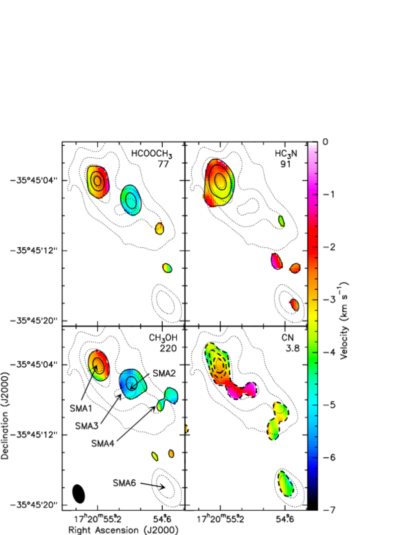
Figure 9.— In each panel, the color scale shows the first moment map of the indicated molecular line, while the solid black contours depict the integrated intensity image of the line emission. In the case of CN, the dashed contours indicate that the line appears in absorption. The levels are: HCOOCH₃= 2.1, 6.3, 10.5 Jy km s^-1; HC₃N= 2.55, 5.95, 14.45 Jy km s^-1; CH₃OH= 1.89, 5.67 Jy km s^-1; CN = -1.2, -2.4, -3.6 Jy km s^-1. In each panel, the thin dotted contours show the 1.3 mm continuum emission (levels = 60, 180, 390, and 900 mJy beam^-1). The numbers below each molecular name is the $E_{\rm lower}$ of the transition in units of cm^-1.

Figure 10.— (a) Sample spectra toward the 1.3 mm continuum peak of SMA1. (b) Sample spectra toward the 1.3 mm continuum peak of SMA2. In both plots the dashed line indicates the $V_{lsr}$ and the numbers in parenthesis under the molecule names are the lower state energy in cm^-1. In (a) the two dotted lines indicate the velocity of the peak red and blueshifted H₂CO ($E_{l}=7$ cm^-1) emission. In (b) the dotted line indicates the velocity of the peak blueshifted H₂CO ($E_{l}=7$ cm^-1) emission and the dot-dashed line indicates the velocity of maximum CN absorption.

3.6. Mid-infrared Emission

Figure 11 shows a three color mid-IR image of the I(N) region with methanol maser positions and integrated SiO and 1.3 mm continuum contours superposed. The extended 4.5 $\mu$m emission to the SW of the I(N) continuum has been reported previously by Hunter et al. (2006). In addition, a weak region of predominantly 4.5 $\mu$m emission is also visible between the SMA6 continuum peak and the arc of 44 GHz CH₃OH masers $5\arcsec$ to the SW; this region is coincident with the blueshifted side of the SMA6 outflow (Fig. 7c). Clumpy knots of extended 4.5 $\mu$m emission are also present to the NE of SMA1, and in the vicinity of SMA7. We also present for the first time, an unresolved source of 24 $\mu$m emission located $\sim 2\arcsec$ SW of SMA4. This figure demonstrates that with the exception of extended 4.5 $\mu$m emission, and a single source of 24 $\mu$m emission, NGC 6334 I(N) is relatively dim in the mid-IR. Indeed, SMA4 appears to be the only millimeter continuum source directly associated with a mid-IR source. In contrast, the bright haze of red emission in the SW corner of Fig. 11 emanates from the periphery of the saturated mid-IR bright protocluster NGC 6334 I. The nature of the mid-IR emission is discussed in detail in §4.1 and §4.2.

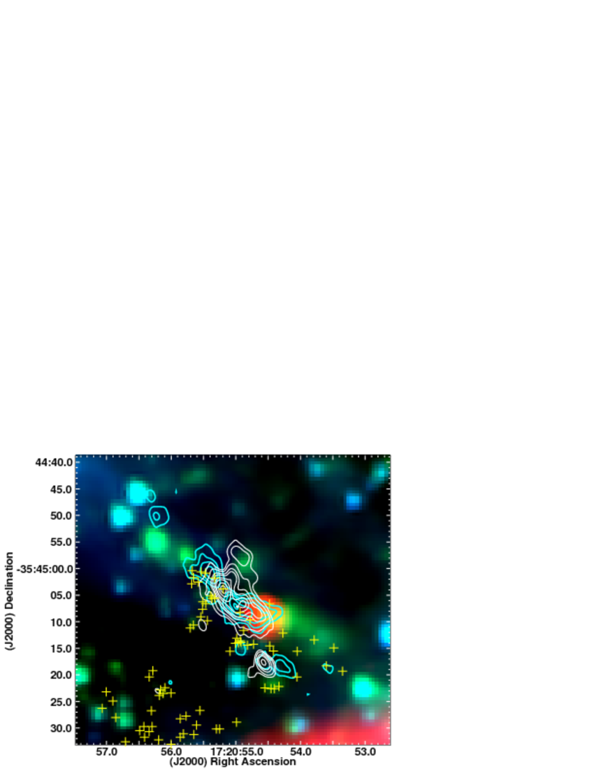
Figure 11.— Spitzer 3-color image with RGB mapped to 24, 4.5, and 3.6 $\mu$m. White 1.3 mm continuum and cyan SiO integrated intensity contours are overlaid, along with yellow $+$ symbols showing the locations of the 44 GHz CH₃OH masers. The 1.3 mm continuum contour levels are the same as Fig. 1, and the SiO (5–4) integrated emission contour levels are 6, 10, 14, 20, 26 mJy beam^-1*km s^-1.

4. DISCUSSION

4.1. Presence of Multiple Outflows

Due to the ubiquity of bipolar outflows from protostars, one would expect to find multiple outflows in a protostellar cluster. As discussed in Cyganowski et al. (2008) (and references therein), the 4.5 $\mu$m IRAC passband can be dominated by molecular line emission from H₂ and vibrationally-excited CO in regions of strong shocks such as those found in massive molecular outflows. To the NE of SMA1, the extended 4.5 $\mu$m emission appears to be an extension of the large-scale NE-SW SMA1 outflow traced by SiO and other tracers of the extended emission (see Figs. 6,7a,11). To the south where the outflows from SMA1 and SMA4 (westward flow) overlap, it is unclear which outflow the 4.5 $\mu$m emission is arising from. Interestingly, the 4.5 $\mu$m emission extends further than the SiO does to the west and SW. As described in §3.5, SMA2 may harbor a more or less pole-on outflow as traced by blueshifted H₂O masers and possibly H₂CO. As described in §3.6 and §3.7, a smaller scale NE-SW outflow also appears to emanate from SMA6, with blueshifted SiO and 44 GHz CH₃OH maser emission located to the south coincident with 4.5 $\mu$m emission (Figs. 7c,11).

The ATCA molecular line data reported by Beuther et al. (2007, 2008) (HCN(1–0) and NH₃ for example) show good overall morphological agreement with the largescale emission emanating from SMA1 observed with the SMA (see for example Figs. 6,7,11). In particular, the complex kinematics of the extended emission were also noted by Beuther et al. and ascribed to possible precession. This idea is in good agreement with the discovery of a possible tight binary in SMA1b and SMA1d (separated by $\gtrsim 800$ AU) if these two sources do in fact represent two different protostars (see for example Chandler et al., 2005; Anglada et al., 2007; Cunningham et al., 2009). Although Figs. 6,7a,b,c,11 show SiO and other molecules in the vicinity of SMA6, Beuther et al. (2007, 2008) did not detect any significant molecular emission in this region. However, SMA6 was near the edge of the ATCA primary beam.

It is notable that the orientation of the NE-SW outflow inferred to originate from SMA1 is different from the largescale SE-NW outflow direction inferred from single-dish SiO(5–4) data with $23\arcsec$ resolution presented by Megeath & Tieftrunk (1999). In their single dish data, blueshifted emission is located to the SE of I(N) in the vicinity of SM2 (Fig. 4.3), while blueshifted and redshifted emission overlap in the vicinity of I(N). Toward I(N), the P-V diagram presented by Megeath & Tieftrunk (1999) shows good agreement with the velocity range observed in the SMA SiO(5–4) data ($-30$ to $+17$ km s^-1, Fig. 7a,b), and indeed the SEST data did not have sufficient spatial resolution to resolve the SMA sizescale flow from SMA1. Moreover, Megeath & Tieftrunk (1999) also observe a clump of shocked 2.2 $\mu$m H₂ emission coincident with the northeastern lobe of the SMA1 outflow and extended 4.5 $\mu$m emission. Thus, it seems likely that the single outflow reported by Megeath & Tieftrunk (1999), is in fact at least two outflows – one consistent with the NE-SW flow detected by the SMA and a second in the vicinity of SM2 and the C1 and C2 water masers. This second outflow would also explain the widespread 44 GHz CH₃OH maser emission observed in this region. While this seems the most probable interpretation of the data, it is also possible that spatial filtering of the SMA data on sizescales $\gtrsim 20\arcsec$ have played a role in the apparent discrepancy. Unfortunately, the SM2 area is beyond the primary beam of the SMA observations, so additional data will be required to explore this region of activity further.

4.2. Nature of Mid-infrared Emission

To assess the nature of the mid-IR emission in more detail we analyzed the 1-8 $\mu$m flux densities of several knots in the vicinity of I(N) that morphologically appear to be dominated by shock line emission. We included data from the Spitzer IRAC bands (see for example Ybarra & Lada, 2009), but also near-infrared $J$, $H$, and $K_{s}$ fluxes (see for example Smith, 1995). To derive the physical conditions, we have implemented a set of shock models similar to that of Ybarra & Lada (2009) (see also Neufeld & Yuan, 2008; Smith & Rosen, 2005; Smith et al., 2006). We calculate the equilibrium excitation of molecular hydrogen (H₂) in a grid of temperatures (1000-5000 K) and densities (10²-10⁶ cm^-3) using the escape probability code Radex (van der Tak et al., 2007, since the optical depths are low, the escape probability formalism is not critical, but the code was still very useful to read the extensive tables of molecular data). We use excitation rates from collisions with H₂ and He from Le Bourlot et al. (1999, 2002) including reactive collisions as prescribed therein, and from collisions with H from Wrathmall et al. (2007). Quadrupole transition probabilities are from Wolniewicz et al. (1998). We convolve the line intensities with Spitzer (Reach et al., 2005) and 2MASS filter transmission profiles to calculate band-average fluxes as specified in appendix A of Robitaille et al. (2007).

The analysis of the shocked emission is complicated by diffuse PAH emission, especially in the 5.8 and 8.0 $\mu$m images. We performed several different background subtractions to attempt to isolate the H₂ emission, with the assumption that most of the emission at 4.5 $\mu$m is H₂ (there are no PAH emission features in that band). Naturally this decomposition is subject to uncertainty, so the precision of shock physical parameters is limted by this observational fact. We find that the near and mid-IR broadband flux ratios are most consistent with the hottest post-shock temperatures ($\sim$4000K), indicating that these are strong shocks as would be expected from a powerful massive stellar outflow. The density in the shock cooling zone is harder to constrain because density changes the broadband flux ratios less than does temperature (see Fig. 2 in Ybarra & Lada, 2009), and because foreground extinction can mimic a decrease in emitting material density. The fluxes here are broadly consistent with densities of 10³–$10^{5}$ cm^-3. Once we have constrained the physical parameters in the H₂ emitting zone, we can translate mid-infrared fluxes into total shock luminosity. For shock recombination zones (T$\simeq$4000K) our models indicate that 6% of the total H₂ line emission comes out in the IRAC 4.5 $\mu$m band. The NGC6334I(N) outflow emits 15$\pm$3 Jy over 100$\pm$20 square arcseconds (sum of both lobes). At a distance of 1.7 kpc, that corresponds to 2300$\pm$300 L_☉ total luminosity in shocked molecular hydrogen, with an average column density of 3.5$\pm$0.5$\times$10²¹cm^-2, for a total of 0.1 M_☉ of hot shocked material (that which is emitting at the highest temperatures – a much larger mass of cooler and entrained material is present in the outflow as well, simply not emitting in the near infrared).

SMA4 is the only source in I(N) associated with 6.7 GHz CH₃OH masers (see §3.3.2), and in §3.6 we report the detection of a 24 $\mu$m source $2\arcsec$ to the SW of the 1.3 mm continuum peak. Class II 6.7 GHz CH₃OH masers are thought to be radiatively pumped by warm dust, and are found almost exclusively in regions of massive star formation (Cragg et al., 2002, 2005; Minier et al., 2003), providing strong evidence that SMA4 is a massive protostar. Two scenarios exist for the nature of the 24 $\mu$m emission: (1) it may trace emission from hot dust near a central protostar and is the 24 $\mu$m counterpart to SMA4 or (2) it traces emission from hot dust in the walls of the cavity formed by the outflow traced by extended 4.5 $\mu$m and molecular line emission, as well as 44 GHz methanol masers W/SW of SMA4. Recent work by De Buizer et al. (2005); De Buizer (2007) favor the latter interpretation. Higher-resolution mid-infrared data would help to distinguish between these possibilities for SMA4. The 24 $\mu$m flux is 0.45$\pm$0.04 Jy, or 2 $L_{\sun}$ (just in the 24 $\mu$m band). Protostars emit roughly 5% of their luminosity in the 24 $\mu$m band over a relatively large range of evolutionary state, so if this source represents a significant fraction of the luminosity of the driving protostar, the latter would have an approximate luminosity of only about 40 $L_{\sun}$. This low luminosity lends support to the interpretation that the 24 $\mu$m emission is coming from hot dust away from the central source, such as on an outflow cavity, and that the driving source itself is still highly embedded and extinguished even at 24 $\mu$m.

4.3. What are the 44 GHz Methanol Masers Tracing?

The 44 GHz Class I CH₃OH maser line is often found in regions of high-mass star formation (Haschick et al., 1990; Slysh et al., 1994; Kurtz et al., 2004; Val’Tts & Larionov, 2007; Pratap et al., 2008). Like other Class I masers (Plambeck & Menten, 1990), it is often found separated from compact H ii regions and in many cases appears to be associated with shocked gas created by bipolar outflows (e.g. Kurtz et al., 2004; Sandell et al., 2005). While this maser has been found within other millimeter protoclusters such as S255N and G31.41+0.31 (Cyganowski et al., 2007; Araya et al., 2008), the number and spatial distribution of maser spots is particularly large in NGC 6334 I(N). In all of these studies including the current one, the 44 GHz CH₃OH masers tend to lie within a few km s^-1 of the systemic velocity even though they typically trace powerful outflows. This dichotomy is likely due to the fact that an enhanced column of CH₃OH gas with sufficient velocity coherence along the line-of-sight is most likely to be found where a shock is moving perpendicular to the line-of-sight (i.e. a shock viewed edge-on). The same effect is believed to give rise to the narrow NH₃ (3,3) maser emission located near the ends of the protostellar jet from IRAS 20126+4104 (Zhang et al., 1999).

As described in §4.1, it is possible that the 44 GHz masers located in the SE portion of the observed field of view are associated with an outflow originating from the relatively unexplored region of continuum emission SM2. The discovery of an X-ray source near SM2 indicates that additional cluster members may be present in this area. A more general conclusion can be drawn from the relatively widespread extent ($45^{\prime\prime}\sim 1.2\times 10^{18}$ cm) of 44 GHz maser emission, an extent that is shared by ammonia (1,1) and (2,2) line and 450 $\mu$m continuum emission (see Fig. ). For a single dominant YSO to maintain this region at a conservative minimum temperature of 30 K (the ammonia temperature from Kuiper et al. (1995) and average dust temperature from Sandell (2000)) would require a central luminosity of $5\times 10^{5}$ L_⊙ (e.g. Scoville & Kwan, 1976) which is 30 times higher than the value ($1.7\times 10^{4}$ L_⊙) inferred from the far-infrared spectral energy distribution for this region (Sandell, 2000). Thus, these phenomena must be driven by the collective activity of a number of cluster members.

4.4. Temperatures of the Hot Core Sources SMA1 and SMA2

Figure 12.— Rotation diagrams for the CH₃OH transitions observed for SMA1 (top) and SMA2 (bottom); the fitted temperatures are indicated. The column densities have been corrected for optical depth effects as described in §4.3.

When several transitions of the same molecule spanning a range of energies are observed, temperatures can be inferred from the rotation diagram method (see for example Goldsmith & Langer, 1999), using the relations

$$\frac{N_{u}}{g_{u}}=\frac{3k}{8\pi^{3}\nu g_{I}g_{K}}\frac{1}{\mu^{2}S}\int S_{\nu}dv,$$ (1)

and

$${\rm log}(N_{u}/g_{u})={\rm log}(N_{tot}/Q(T_{rot}))-0.4343E_{u}/kT_{rot},$$ (2)

where k is Boltzmann’s constant, $\nu$ is the frequency, $g_{I}$ and $g_{K}$ are the degeneracies associated with the nuclear spin and k quantum number respectively, $\mu^{2}$ is the square of the dipole matrix element, $S$ is the statistical line strength, $\int S_{\nu}dv$ is the observed integrated intensity of the transition, $N_{tot}$ is the total column density, $Q(T_{rot}$) is the partition function evaluated at the rotation temperature $T_{rot}$, and $E_{u}$ is the upper state energy of the transition. There are seven transitions of CH₃OH detected toward SMA1 and six toward SMA2 (including both A and E type transitions) that can be used for this purpose. The $\int S_{\nu}dv$ for each transition was calculated from Gaussian fits to the line emission at the 1.3 mm continuum peaks. The rotation temperature resulting from a weighted least squares fit to the data is $189\pm 19$ K for SMA1 and $154\pm 14$ K for SMA2.

However, as demonstrated by Goldsmith & Langer (1999) and others, line optical depth can artificially increase the derived rotation temperature if not corrected for. In general the line optical depth in LTE can be calculated from

$$\tau=\frac{8\pi^{3}}{3h}\frac{N_{o}}{g_{o}}\mu^{2}Se^{-E_{u}/kT_{ex}}(e^{h\nu/kT_{rot}}-1)\frac{1}{\Delta v},$$ (3)

where $h$ is Planck’s constant, $N_{o}/g_{o}$ is the column density of the ground state divided by the ground state degeneracy, $T_{ex}$ is the excitation temperature, and $\Delta v$ is the FWHM line width. Then the left hand side of Eq. 2 is modified to ${\rm log}(C_{\tau}N_{u}/g_{u})$ where $C_{\tau}=\tau/(1-e^{-\tau})$. Since we do not know the ground state column density, this equation cannot be used directly to calculate $\tau$ for each transition. Unfortunately, in the I(N) SMA dataset we do not have a suitable isotopologue that can be used to infer the CH₃OH optical depth either (see for example Brogan et al., 2007). Instead, we have iteratively solved for the optical depth and $T_{rot}$ that produces the best $\chi^{2}$ fit to the data (i.e. minimizes the scatter). Using this technique we find the best fit occurs for a $T_{rot}$=$165\pm 9$ K for SMA1 and $T_{rot}$=$145\pm 12$ K for SMA2 (see Figure 12a), and modest optical depths of 1.75 for SMA1 and 0.5 for SMA2 for the observed transition that would have the highest optical depth (CH₃OH-E ($4_{+2,2}-3_{+1,2}$)) at 218.4400 GHz). While not dramatically different from the $T_{rot}$ derived without optical depth correction, these corrected temperatures are clearly more accurate. We do not have enough transitions to do a more sophisticated non-LTE analysis or to compare the results for $A$ and $E$ transitions independently (see for example Sutton et al., 2004). However, we note that for the CH₃OH-E ($5_{+1,4}-4_{+2,2}$) transition (at 216.9456 GHz) which we have in common with the Sutton et al. (2004) methanol survey of the hot core source W3(OH) with comparable spatial resolution, the derived opacity is similar for the two sources (0.45 for SMA1 in I(N) compared to 0.65 for W3(OH)). Indeed the derived temperatures for SMA1 and SMA2 are also very similar to that of W3(OH) ($T_{rot}$ = $140\pm 10$ K, Sutton et al., 2004).

The optical depth implied by the brightness temperature of the strongest methanol transition ($4_{+2,2}-3_{+1,2}$, 24 K) toward SMA1 is only 0.16 assuming that $T_{kin}$=$T_{rot}$=165 K and the emitting region is the size of the LSB synthesized beam ($2\farcs 39\times 1\farcs 55$). An optical depth of 1.75 for this transition implies that the emitting region is actually only $0\farcs 8$ in size (1400 AU). This size is in good agreement with the fitted size ($0\farcs 9\times 0\farcs 7$, PA=$162\arcdeg$) of the integrated intensity measured from the compact, but still strong CH₃OH-A⁺($16_{1,16}-15_{2,13}$) transition ($E_{l}=219.8$ cm^-1)at 227.8147 GHz. This size implies that the hot core region encompasses both SMA1b and SMA1d (see Fig. 2b).

The column densities of CH₃OH for SMA1 and SMA2 are $(1.0\pm 0.4)\times 10^{17}$ cm^-2 and $(5.6\pm 0.6)\times 10^{16}$ cm^-2, respectively, an order of magnitude less than Sutton et al. (2004) find for W3(OH). Sutton et al. (2004) find a CH₃OH abundance of $\sim 2\times 10^{-6}$ for W3(OH). Using single dish observations of infrared dark clouds (IRDCs), Leurini et al. (2007) find abundances an order of magnitude smaller for the IRDC cores. Using this range of abundance and assuming that the hot core size is 1400 AU, we estimate that the H₂ column density is $(0.5-5)\times 10^{23}$ cm^-2 and the H₂ density is $(0.2-2)\times 10^{7}$ cm^-3 for SMA1 and about a factor of two smaller for SMA2.

Using the ATCA, Beuther et al. (2008) observed CH₃CN(5_K–4_K) up to K=4 toward SMA1 and SMA2 and derived a rotation temperature of $T_{rot}$$=170\pm 50$ K for SMA2 in good agreement with our CH$+3$OH measurement ($145\pm 12$ K). The optical depth in SMA1 was too high to obtain a CH₃CN $T_{rot}$ for SMA1 in good agreement with our finding that this source has a higher column density than SMA2. Also using the ATCA, Beuther et al. (2007) detected NH₃ (5,5), and (6,6) emission toward both SMA1 and SMA2 confirming that $T_{k}$ is greater than 100 K, though it was not possible to derive more accurate estimates from those data.

4.5. The Nature of the 1.3 mm Sources

4.5.1 Spectral Energy Distributions

Figure 13.— Spectral energy distributions for sources SMA1, SMA4, and SMA6. For SMA1, the sum of the emission of SMA1a,b,c, and d are shown as solid squares, while the flux density as a function of frequency for SMA1b is shown as open squares for $\nu\leq 43$ GHz. Open squares are also used for the $\nu\leq 43$ GHz emission for SMA4 to indicate that they may not be from the same source as the higher frequency data, the fits in this case assume case 3 described in S4.5.1. Emission models from dust are shown as dashed (or dot-dash in the case of SMA1b) lines, while emission models for free-free emission are shown as dotted lines. For SMA1 the sum of the dust and free-free emission models, described in detail in §4.4.1, is shown as a solid line.

Because no higher frequency arcsecond-resolution data exist on this region, the determination of the nature of the 1.3 mm sources hinges entirely upon accurate measurements of their spectral index toward longer wavelengths (thus motivating our careful re-reduction of the available data). The comparatively poor angular resolution of the current 1.3 and 3.4 mm data compared to the 7 mm, 1.3 cm, and 3.6 cm data makes it challenging to disentangle the free-free versus dust contributions to these sources. Figure 13 shows the spectral energy distributions (SEDs) of SMA1, SMA4, and SMA6 based on the flux densities provided in Table 1. The different resolutions of the different datasets are definitely a concern. However, in many cases the emission does not appear to be resolved even in the highest resolution observations of SMA4, and to some degree SMA6. In that case, as long as no significant emission is resolved out, the data will still be comparable despite the differing resolutions. Caveats for a few sources are described in detail below.

For SMA1, which contains at least four components at the longer wavelengths, we show both the integrated emission over the whole SMA1 region, and SMA1b by itself at wavelengths longer than 7 mm for comparison. The integrated emission from SMA1 shows evidence for both a free-free and an optically thin dust component. The integrated dust spectral index of $\alpha_{dust}=3.8\pm 0.1$ ($S_{\nu}\propto\nu^{\alpha}$) was determined by a linear least-squares fit to the three flux densities from 7 mm to 1.3 mm (for SMA1 at 7 mm this is the sum of emission from SMA1a,b,c, and d; the free-free contribution is an order of magnitude smaller and hence negligible in the dust fit). On smaller scales, we also find that the 7 mm emission from SMA1b is dominated by dust, while the 3.6 cm emission is consistent with optically-thin free-free emission with a spectral index of $\nu^{-0.1}$, such as that from an H ii region with an electron density of $3\times 10^{4}$ cm^-3, temperature of 10000 K and a diameter of $0.3\arcsec$ (510 AU). At the intermediate wavelength of 1.3 cm, these two emission mechanisms are comparable for SMA1b, with $\approx 30$% of the emission arising from dust. This is a notable result since 1.3 cm data are typically assumed to be free of dust.

The emission from SMA1a may all be due to dust since it is not detected longward of 7 mm; the $3\sigma$ 1.3 cm upper limit of $\sim 0.18$ mJy implies that the spectral index must be $>2.4$. In contrast, both SMA1c and SMA1d are detected at 1.3 cm and have a 1.3 cm to 7 mm spectral index of $sim2$. This spectral index could be due to optically thick dust emission which seems very unlikely at these wavelengths, optically thick free-free emission such as one might observe around a very dense hypercompact H ii region, or a combination of optically thin free-free and dust emission. If we take the total observed flux density of SMA1 at 1.3 cm (1.07 mJy, i.e. the sum of SMA1a upper limit and SMA1b,c,and d detections) and subtract the total dust model (0.50 mJy) and the SMA1b free-free emission model (0.35 mJy), we find that 0.22 mJy remains, suggesting that the integrated dust model cannot account for all of the SMA1c+SMA1d emission. Thus, one or both of SMA1c and SMA1d must have a weak free-free component, and since these objects have 1.3 cm flux densities of 0.27 and 0.30 mJy, respectively (greater than the residual), both must also have a dust component. If all of the free-free residual (0.22 mJy) belonged to either SMA1c or SMA1d, the $3\sigma$ 3.6 cm upper limit of $\sim 0.12$ mJy implies a free-free spectral index $>0.6$, consistent with a thermal jet, stellar wind, or hypercompact H ii region. If instead the residual free-free emission is about equally split between SMA1c and SMA1d both could harbor small optically thin H ii regions in addition to a dust component.

Understanding the nature of SMA4 is complicated by the lack of positional agreement between the 1.3 - 3.4 mm data compared to the longer wavelength data (3.6 cm, 1.3 cm, and 7 mm offset $\sim 0\farcs 4$ to the NW; Fig. 3). From the spectral break in the SMA4 SED around 7 mm shown in Fig. 13 it is clear that both dust and free-free emission is present in this region. The spectral index of the SMA4 emission between 1.3 and 3.4 mm is $\alpha_{dust}=4.4\pm 0.3$, while the spectral index between 3.6 cm and 7 mm is $\alpha_{ff}=0.63\pm 0.25$ suggesting either a hypercompact H ii region with a turnover around 7 mm (see for example the review by Lizano, 2008), or a thermal jet/stellar wind (Reynolds, 1986). Overall, the data are consistent with the following three possibilities: (1) the emission all arises from the same source which contains both dust and a hypercompact H ii region (i.e. the position offsets are just within the combined position uncertainties); (2) Two sources are present: one is a compact dust source with no detectable free-free emission (1.3 - 3.4 mm emission) and the other (7 mm - 3.6 cm emission) is a hypercompact H ii region ($\gtrsim 700$ AU away); or (3) the free-free emission arises from a one-sided thermal jet driven by the dust source of case (2). If we assume case (1) and fit the centimeter wavelength emission from SMA4 after extrapolating and subtracting the dust spectrum, we find that a free-free component with a constant density, temperature, and size of $1.2\times 10^{6}$ cm^-3, 8000 K, and 53 AU best approximates the 3.6 and 1.3 cm data points (see Hunter et al., 2008, for the details of the free-free emission model). However, this model overpredicts the 7 mm flux density by a significant margin. More sophisticated free-free emission models, such as those with a density gradient and/or a shell geometry, may provide a better match to the 7 mm data (see for example Avalos et al., 2006). However, the present data are insufficient in angular resolution and number of spectral measurements to meaningfully constrain a more detailed model. For case (2), it is even more difficult to fit the 7 mm data with a hypercompact H ii region model because the spectrum from 3.6 cm to 7 mm is so linear, and yet not steep enough to still be optically thick (i.e. spectral index of 2). Thus, case (3) seems to best fit the current data (see Fig. 13, with the 3.6 cm to 7 mm data having a typical jet or stellar wind spectral index ($\alpha_{ff}=0.6$ Reynolds, 1986), and no dust component. We note that in the jet interpretation for the cm-$\lambda$ emission (case 3) the $\sim 0\farcs 4$ offset of the cm-$\lambda$ to the west is in good agreement with the fact that a westward outflow appears to emanate from SMA4.

Although there is an offset $\sim 0\farcs 3$ to the north between the 7 mm and 1.3 mm emission toward SMA6, the fact that the shape of the continuum contours at these two wavelengths is similar, and most of the apparent offset is along the long axis of the 1.3 mm beam makes it quite plausible that they are in fact coincident (also note that the offset is not in the same direction as that of SMA4). Indeed, the emission from SMA6 can be explained completely by optically-thin dust emission (at the current level of sensitivity). The dust spectral index from a linear fit to the three flux densities from 7 mm to 1.3 mm is $\alpha=4.0\pm 0.2$. If we assume all the 1.3 mm emission arises from a region with the size measured from the higher resolution 7 mm image, ($0\farcs 9\times 0\farcs 7$), the brightness temperature is $T_{b}=25$ K setting a lower limit on the dust temperature. There is a hint of a break towards a flatter spectral index at 1.3 mm for SMA6, as would be expected if the dust emission were becoming optically thick, but higher frequency data are required to confirm this trend.

SMA2 and SMA3 are the only strong, compact millimeter sources not to be detected at wavelengths longward of 3.4 mm. Between 1.3 and 3.4 mm the spectral index of SMA2 is $\alpha=4.0\pm 0.3$, and that of SMA3 is $\alpha=4.3\pm 0.3$, consistent with optically thin dust emission. Extrapolating these spectral indices to 7 mm, we would have expected to detect SMA2 and SMA3 at the 1.4 and 0.9 mJy level, respectively (amounting to $7\sigma$ and $4.5\sigma$) if the emission were unresolved at 7 mm. The sizes derived for SMA2 and SMA3 at 1.3 mm are $2\farcs 1\times 1\farcs 3$ and $2\farcs 5\times 1\farcs 9$. If these are the true sizes of the emitting regions, the peak 7 mm intensity would be diminished by a factor of $\sim 10$ over that predicted here, plausibly explaining the non-detections. The emission denoted VLA3 is only detected at 7 mm, and thus its nature is very uncertain. The non-detection of VLA3 at 1.3 cm implies that its spectral index is $>2$, and we estimate a 1.3 mm upper limit of $\sim 150$ mJy suggesting that its spectral index must also be less than $\sim 3$. These limits suggest that VLA3 is predominately due to dust emission, but contribution from a hypercompact H ii region cannot be excluded.

In summary, of the nine compact sources detected in I(N), all appear to have a dust component. Four of these sources (SMA1b, SMA1c, SMA1d, and SMA4) also show evidence for free-free emission at our current level of sensitivity. Three sources (SMA1b, SMA1d, and SMA2) and possibly a fourth (SMA4) show modest hot core molecular line emission, also suggesting the presence of a central powering source. One source with neither free-free nor hot core emission does appear to be powering an outflow (SMA6). From this circumstantial evidence it appears that at least six of the compact sources may harbor a central source. However, as described by Zinnecker & Yorke (2007), in deeply embedded regions it is extraordinarily difficult to determine whether a massive protostar or zero age main sequence star (ZAMS) has formed, as this designation is dependent upon detecting the source in the near-IR (a wavelength regime in which I(N) is still obscured). In principle, the detection of free-free emission is often taken as indicative of at least an early B-type star. However, even the presence of free-free emission is ambiguous since the accretion luminosity itself can be sufficient to ionize the gas around a protostar. Thus, while it is clear that a number of massive to intermediate stars are forming in I(N), the exact number and evolutionary state is uncertain.

A few comments on the previously published flux measurements for these sources are in order. When the more accurate absolute flux calibration presented here for the original Carral et al. (2002) 3.6 cm data is taken into account, the agreement for SMA4 is quite good. However, it is unclear why the detection of SMA1b was not reported by these authors, since it is 1.6 times brighter than SMA4. We obtain 7 mm flux densities between 2.2 (SMA6) to 8 (SMA1a) times smaller than those reported by Rodríguez et al. (2007), though our 1.3 cm flux densities are comparable. This discrepancy comes in spite of the fact that the flux densities derived for the phase calibrators at both 7 and 1.3 cm are within $2\%$ for our reduction compared to that reported in Rodríguez et al. (2007). As described in §2.2.3, continuum emission from the strong ultracompact H ii region in source I causes significant contamination of the I(N) region if not included in the cleaning; however our detailed tests suggest that at most it could erroneously increase the integrated fluxes by a factor of $\sim 2$, and thus cannot account for the large discrepancy. In addition, the integrated flux densities reported in Rodríguez et al. (2007) do not appear consistent with the contour levels plotted in their Figures 2 and 3, indeed the peak values are reasonably consistent with those reported here so the problem may have occurred in their integrated Gaussian fits. Finally, our re-imaging of the 3.4 mm data from Beuther et al. (2008) has increased the peak flux densities by a factor of about 1.5 due to our self-calibration and correction for the primary beam attenuation.

4.5.2 Mass estimates from the dust emission

In Table 6 we give estimates for the gas mass $M_{gas}$, molecular hydrogen column density $N_{H_{2}}$, and molecular hydrogen density $n_{H_{2}}$ for all seven 1.3 mm dust sources. It should be noted that if a protostar or zero age main sequence star has already formed, the millimeter data is only sensitive to the circum-(proto)stellar material. The gas masses were calculated from

$$M_{gas}=\frac{3.24\times 10^{-3}S_{\nu}({\rm Jy})D^{2}({\rm kpc})RC_{\tau_{dust}}}{J(\nu,T_{dust})\nu^{3}({\rm THz})\kappa_{\nu}}~{}{\rm M_{\odot}},$$ (4)

where $S_{\nu}$ is the integrated flux density from Table 1, $D$ is the distance (assumed to be 1.7 kpc), $R$ is the gas to dust ratio (assumed to be 100), $J(\nu,T)=1/({\rm exp}(h\nu/T_{dust}k)-1)$, and $C_{dust}$ is the correction factor for the dust opacity $C_{\tau_{dust}}=\tau_{dust}/(1-e^{-\tau_{dust}})$. We have used $\kappa_{\rm 1.3~{}mm}=1$ cm² g^-1 which is the average of the dust opacities derived by Ossenkopf & Henning (1994) for the case of thin ice mantles and densities between $10^{6}$ to $10^{8}$ cm^-3 at 1.3 mm. We have estimated a range of dust temperatures based on the observed spectral line properties of each source: we use the derived $T_{rot}$ values calculated in §4.4 for SMA1 and SMA2, and a lower temperature range for SMA3 to SMA7 based on the non-detection of hot core spectral lines towards these sources. The column densities were estimated from

$$N_{H_{2}}=\frac{2.4\times 10^{30}S_{\nu}({\rm Jy})RC_{\tau_{dust}}}{J(\nu,T_{dust})\nu^{3}({\rm THz})\theta_{1}(\arcsec)\theta_{2}(\arcsec)\kappa_{\nu}}~{}{\rm cm}^{-2},$$ (5)

where $\theta_{1}$ and $\theta_{2}$ are the fitted sizes from Table 1. The $n_{H_{2}}$ was calculated by dividing $N_{H_{2}}$ by the geometric mean of the fitted size, assuming a distance of 1.7 kpc. The estimated dust masses are similar to those reported in Hunter et al. (2006) when the differences in absolute flux calibration and assumed dust temperatures are taken into account. As with all such estimates, the $M_{gas}$, $N_{H_{2}}$, $n_{H_{2}}$ reported in Table 6 are uncertain to at least a factor of 2. The total mass estimated for the compact emission of I(N) is between 89 and 232 M_⊙. These dust emission based masses do not include the mass of any protostars or ZAMSs that may already have formed within the compact cores. It is also notable that Matthews et al. (2008) estimate that the mass of the whole I(N) core is $\sim 2780$ M_⊙, so there is still a considerable reservoir of material that has not yet collapsed.

The values for SMA1 are particularly uncertain because the current 1.3 mm resolution is insufficient to distinguish between the four dust sources detected at 7 mm (SMA1a, SMA1b, SMA1c, and SMA1d). This unresolved structure makes the apparent size of this source quite large – significantly affecting all derived quantities. For example, if we assume that the majority of dust emission comes from a region half the size (in both directions) of the current fit ($2\farcs 8\times 1\farcs 9$), the mass increases only a little (due to increase in $C_{\tau_{dust}}$), but $N_{H_{2}}$ and $n_{H_{2}}$ both increase by about an order of magnitude. An additional source of uncertainty is the $T_{dust}$. As described in §4.3, the hot core line emission appears to arise from a $0\farcs 8$ region encompassing only SMA1b and SMA1d. Thus, the $T_{dust}$ range derived from the CH₃OH rotation diagram may not be appropriate for SMA1a or SMA1c. Using $\kappa_{\rm 7~{}mm}=0.05$ cm² g^-1 (obtained by scaling $\kappa_{\rm 1.3~{}mm}=1$ by (7 mm/1.3 mm)^-β with $\beta=\alpha_{dust}-2$ where $\alpha_{dust}=3.8$ from Fig. 13), and $T_{dust}=155-175$ K we find that the sum of the masses derived for SMA1a,b,c, and d at 7 mm is 20 - 18 M_⊙ in good agreement with the 1.3 mm estimate for SMA1 (16 - 14 M_⊙). Indeed, the agreement is nearly perfect if we assume that the dust emission at 1.3 mm arises from an area $5\times$ smaller than the current size estimate (i.e. Table 1), which is certainly plausible. Higher resolution 1.3 mm observations are required to better constrain the temperatures of SMA1a and SMA1c, as well as the sizes of all four SMA1 sources.

4.6. Evidence for Accretion and Infall Around SMA1?

As described in §3.4, a SE-NW velocity gradient of $\sim 5$ km s^-1 is observed toward SMA1 in some (but not all) of the species with compact emission (a similar gradient was inferred from a double peaked NH₃(6,6) profile by Beuther et al., 2007). Since the gradient is barely spatially resolved with the current SMA resolution, the nature of this gradient is unclear. Its direction is more or less perpendicular to the large scale NE-SW outflow suggestive of a possible disk interpretation, but it also has the same orientation as a line joining the SMA1b and SMA1d sources, and thus could simply represent unresolved emission from these two sources if they have different systemic velocities (as was found for CephA-East in a similar situation by Brogan et al., 2007). We note that this velocity gradient was not observed in the CH₃CN(5_K–4_K) transitions observed by Beuther et al. (2008) with the ATCA. Higher spatial resolution data will be needed to further explore this velocity gradient.

As described in §3.5.2, there is a trend of increasingly redshifted absorption with increasing line excitation temperature toward SMA1, using CN ($E_{l}$=3.8 cm^-1), H₂CO($E_{l}$=7 cm^-1), and H₂CO ($E_{l}$=40 cm^-1) as tracers (see Fig. 10a). In §4.3 we find that the hot core of SMA1 has a temperature of $165\pm 9$ K, demonstrating that this source is definitely centrally heated, suggesting higher excitation lines will be found closer to the center. We suggest that the observed redshift/temperature trend is tracing infall that is accelerating with depth into the core. It would be very interesting to follow-up this tentative result with higher angular and spectral resolution. In particular if the continuum emission were resolved, one could be assured that all emission/absorption originates from only the front side of the source, removing any ambiguities (see for example Chandler et al., 2005).

4.7. The Location of the Protocluster

Finally, it is interesting to note that the massive protocluster appears to be forming near the northwestern edge of the parent cloud rather than toward the center. This offset is apparent in both the JCMT 450 $\mu$m continuum image (Fig. 4.3) and in the ammonia (1,1) and (2,2) images (Beuther et al., 2005). It is notable that the archival SCUBA 450 $\mu$m images recently produced by Di Francesco et al. (2008) show very good positional agreement (to within $3\arcsec$) with the earlier images produced by Sandell (2000) (and shown in Fig. 4.3). The ridge of dust emission between the protocluster and the masers associated with the SM2 continuum source coincides with a dark area in the Spitzer 3-color image (Fig. 11), i.e. an infrared dark cloud (IRDC; see for example Egan et al., 1998). Clearly this region is optically-thick in the mid-infrared, and contains a significant amount of potential star-forming material. Future observations with broader bandwidth and greater sensitivity with the EVLA and ALMA may reveal whether this area is truly quiescent or contains embedded, pre-protostellar cores.

5. CONCLUSIONS

Our multiwavelength radio through near-infrared investigation of the massive protocluster NGC6334I(N) provides new morphological and quantitative detail on the star formation activity of the individual massive cores. We show that I(N) is undergoing copious massive star formation with many of the dominant sources detected only at millimeter wavelengths. The principal source SMA1 is resolved into four components of dust and/or free-free emission (SMA1a, b, c, and d). Delineated by centimeter continuum and water masers, SMA1b and SMA1d form a close central pair ($\gtrsim 800$ AU) which powers a hot core ($T_{rot}$=$165\pm 9$ K) of molecular line emission and likely drives the dominant large-scale bipolar outflow which exhibits evidence of precession. We find a spatially unresolved $\sim 5$ km s^-1 velocity gradient across SMA1 (encompassing all 4 subarcsecond components). The origin of this velocity gradient (rotation, or cluster kinematics) requires higher resolution millimeter wavelength follow-up. We also detect possible infall that is accelerating with depth into the SMA1 core; higher angular resolution is also required to confirm this finding. The mass of gas around SMA1 as traced by compact emission is estimated to be $\sim 15$ M_⊙, but if this core is still actively accreting, this may grow significantly larger in the future.

A weaker hot core ($T_{rot}$=$145\pm 12$ K) is found toward SMA2 which also exhibits redshifted CN absorption along with with highly blueshifted water masers, suggesting simultaneous infall and outflow in this source. SMA4 consists of a dust core with a probable centimeter jet, water maser emission, and blueshifted SiO emanating to the west suggesting an outflow which terminates in a reflection nebula traced by the 24 $\mu$m source. Mostly lacking in molecular lines, SMA6 exhibits a centimeter-millimeter SED consistent with pure dust emission and drives an outflow traced by SiO, CO and 44 GHz methanol masers. Overall, the narrow velocity range and spatial arrangement of the 44 GHz methanol masers with respect to the protocluster members are consistent with their origin in low-velocity gas impacted by outflows from these objects.

The presence of multiple outflows in the region suggests that many protostars are forming simultaneously. At the same time, the variety of phenomena associated with the individual cluster members suggests a spread in either age or total luminosity. Also of interest is the spread in systemic velocities observed between the cluster members, this spread is at least 2.5 km s^-1 and may provide an important clue about the dynamics of cluster formation. A more quantitative assessment of these key properties will require broader wavelength coverage to better constrain the SEDs, and more sensitive continuum and line observations enabled by the EVLA and ALMA in the near future. At the same time, a deeper exploration of the mostly featureless, infrared-dark region between the protocluster and SM2 may prove fruitful in the study of pre-protostellar cores.

Table 1Observed Properties of Compact Continuum Sources

	Centroid positiona		Peakb	Integratedb	Estimated
Source	RA (J2000)	Dec (J2000)	Intensity	Flux Density	Size
	$\alpha$ (${}^{\rm h}~{}~{}^{\rm m}~{}~{}^{\rm s}$)	$\delta$ (${}^{\circ}~{}~{}{{}^{\prime}}~{}~{}{{}^{\prime\prime}}$)	(mJy beam-1)	(mJy)	($\arcsec\times\arcsec$ [P.A. $\arcdeg$])
1.3 Millimeterc
SMA1	17 20 55.188	-35 45 03.92	826 (6)	2550(50)	$2.8\times 1.9~{}[23]$
SMA2	17 20 54.890	-35 45 06.71	324 (6)	980 (25)	$2.1\times 1.3~{}[137]$
SMA3	17 20 54.990	-35 45 07.29	258 (6)	1060 (31)	$2.5\times 1.9~{}[9]$
SMA4	17 20 54.667	-35 45 08.38	141 (6)	770 (40)	$3.0\times 1.5~{}[41]$
SMA5	17 20 55.054	-35 45 01.49	140 (6)	440 (100)	$\leq 2.0$
SMA6	17 20 54.563	-35 45 17.71	282 (9)	600 (29)	$2.2\times 0.9~{}[38]$
SMA7	17 20 54.931	-35 44 57.79	60 (6)	360 (40)	$3.2\times 2.3~{}[47]$
3.4 Millimetere,f
SMA1	17 20 55.194	-35 45 03.79	55 (5)	90 (10)	$\leq 3.0$
SMA2	17 20 54.86	-35 45 06.5	24 (5)	$\cdots$	$<1.6$
SMA3	17 20 54.99	-35 45 07.0	20 (5)	$\cdots$	$<1.6$
SMA4d	17 20 54.69	-35 45 07.5	13 (3)	$\cdots$	$<1.6$
SMA5d	17 20 55.04	-35 45 01.3	15 (3)	$\cdots$	$<1.6$
SMA6	17 20 54.588	-35 45 17.86	31 (3)	$\cdots$	$<1.6$
7 Millimeter
SMA1a	17 20 55.150	-35 45 05.28	0.9 (0.2)	1.7 (0.3)	$\leq 1$
SMA1b	17 20 55.194	-35 45 03.50	1.3 (0.2)	2.5 (0.4)	$0.6\times 0.4~{}[130]$
SMA1c	17 20 55.275	-35 45 02.46	0.9 (0.2)	$\cdots$	$<0.4$
SMA1dd	17 20 55.229	-35 45 03.68	1.0 (0.2)	$\cdots$	$<0.4$
VLA3d	17 20 54.999	-35 45 06.48	1.0 (0.2)	1.8 (0.3)	$\leq 1$
SMA4d	17 20 54.624	-35 45 08.24	0.7 (0.2)	$\cdots$	$<0.4$
SMA6	17 20 54.585	-35 45 16.97	1.3 (0.2)	1.7 (0.3)	$0.9\times 0.7~{}[15]$
1.3 Centimeter
SMA1a	$\cdots$	$\cdots$	$<0.18$ (0.06)	$\cdots$	$\cdots$
SMA1b	17 20 55.191	-35 45 03.53	0.50 (0.07)	$\cdots$	$<0.3$
SMA1c	17 20 55.270	-35 45 02.45	0.27 (0.06)	$\cdots$	$<0.4$
SMA1dd	17 20 55.229	-35 45 03.68	0.30 (0.06)	$\cdots$	$<0.3$
SMA4	17 20 54.623	-35 45 08.25	0.47 (0.07)	$\cdots$	$<0.3$
SMA6	$\cdots$	$\cdots$	$<0.18$ (0.06)	$\cdots$	$\cdots$
3.6 Centimetere
SMA1a	$\cdots$	$\cdots$	$<0.12$ (0.04)	$\cdots$	$\cdots$
SMA1bd	17 20 55.202	-35 45 03.74	0.39 (0.04)	$\cdots$	$<0.3$
SMA1c	$\cdots$	$\cdots$	$<0.12$ (0.04)	$\cdots$	$\cdots$
SMA1d	$\cdots$	$\cdots$	$<0.12$ (0.04)	$\cdots$	$\cdots$
SMA4	17 20 54.623	-35 45 08.25	0.25 (0.04)	$\cdots$	$<0.3$
SMA6	$\cdots$	$\cdots$	$<0.12$ (0.04)	$\cdots$	$\cdots$

Table 222.235 GHz Water Maser Groups in NGC 6334 I(N) 

1 & 17 20 56.058 -35 45 32.59 SM2 (4.50″) $38.3$ $-6.0$ $+5.2$ to $-16.2$
2 17 20 55.650 -35 45 32.48 SM2 (1.78″) $9.2$ $-9.0$ $+7.2$ to $-15.6$
3 17 20 54.600 -35 45 17.27 SMA6 (0.67″) $8.8$ $-2.2$ $+10.4$ to $-12.6$
4 17 20 54.152 -35 45 13.66 - $29.0$ $-2.7$ $-0.7$ to $-4.4$
5 17 20 54.618 -35 45 08.65 SMA4 (2.11″) $17.7$ $+0.2$ $+12.4$ to $-12.9$
6 17 20 54.870 -35 45 06.32 SMA2 (0.55″) $2.7$ $-13.3$ $-4.7$ to $-15.6$
7 17 20 54.819 -35 45 06.18 SMA2 (1.11″) $5.3$ $-0.7$ $+0.2$ to $-1.7$
8 17 20 55.192 -35 45 03.77 SMA1b (0.24″) $78.1$ $-6.3$ $+13.1$ to $-26.8$
9 17 20 55.228 -35 45 03.66 SMA1d (0.02″) $75.7$ $+3.9$ $+5.2$ to $+2.2$
10 17 20 55.147 -35 45 03.78 SMA1 (0.53″) $3.4$ $-8.6$ $-7.7$ to $-9.6$
11 17 20 55.215 -35 45 02.02 SMA1 (1.96″) $5.5$ $-4.4$ $-3.7$ to $-6.3$

Table 322.235 GHz Water Masers Detected in NGC 6334 I(N) 

Velocity	Centroid position		Peak
(km s-1)	R.A. (J2000)	Dec (J2000)	Intensity
	$\alpha$ (${}^{\rm h}~{}~{}^{\rm m}~{}~{}^{\rm s}$)	$\delta$ (${}^{\circ}~{}~{}{{}^{\prime}}~{}~{}{{}^{\prime\prime}}$)	(Jy beam-1)
Group C1
+5.2	17 20 56.0583	-35 45 32.4934	0.384
+4.9	17 20 56.0599	-35 45 32.5678	0.548
+4.5	17 20 56.0585	-35 45 32.5920	0.586
+4.2	17 20 56.0578	-35 45 32.5805	0.893
+3.9	17 20 56.0581	-35 45 32.5797	1.373
+3.5	17 20 56.0586	-35 45 32.5776	1.764
+3.2	17 20 56.0579	-35 45 32.6134	1.675
+2.9	17 20 56.0580	-35 45 32.5594	1.534
+2.5	17 20 56.0581	-35 45 32.5946	1.185
+2.2	17 20 56.0584	-35 45 32.5566	0.934
+1.9	17 20 56.0584	-35 45 32.5619	0.639
+1.6	17 20 56.0614	-35 45 32.4557	0.508
+1.2	17 20 56.0617	-35 45 32.4066	0.381
+0.9	17 20 56.0555	-35 45 32.5404	0.535
+0.6	17 20 56.0579	-35 45 32.5826	0.504
+0.2	17 20 56.0590	-35 45 32.5242	0.497
-0.1	17 20 56.0607	-35 45 32.4663	0.422
-0.4	17 20 56.0584	-35 45 32.5610	0.400
-0.7	17 20 56.0597	-35 45 32.5347	0.558
-1.1	17 20 56.0566	-35 45 32.6202	0.652
-1.4	17 20 56.0588	-35 45 32.5413	0.578
-1.7	17 20 56.0581	-35 45 32.6271	0.749
-2.1	17 20 56.0587	-35 45 32.5695	1.507
-2.4	17 20 56.0582	-35 45 32.5774	3.357
-2.7	17 20 56.0580	-35 45 32.5891	6.453
-3.0	17 20 56.0581	-35 45 32.5907	11.608
-3.4	17 20 56.0579	-35 45 32.5977	16.950
-3.7	17 20 56.0579	-35 45 32.5953	13.072
-4.0	17 20 56.0579	-35 45 32.5929	10.177
-4.4	17 20 56.0579	-35 45 32.5925	13.265
-4.7	17 20 56.0577	-35 45 32.5900	16.513
-5.0	17 20 56.0578	-35 45 32.5893	20.479
-5.4	17 20 56.0578	-35 45 32.5910	28.570
-5.7	17 20 56.0579	-35 45 32.5903	38.006
-6.0	17 20 56.0578	-35 45 32.5935	38.297
-6.3	17 20 56.0578	-35 45 32.5900	28.243
-6.7	17 20 56.0577	-35 45 32.5910	19.718
-7.0	17 20 56.0578	-35 45 32.5912	22.008
-7.3	17 20 56.0578	-35 45 32.5952	31.096
-7.7	17 20 56.0577	-35 45 32.5945	35.008
-8.0	17 20 56.0579	-35 45 32.5918	28.781
-8.3	17 20 56.0579	-35 45 32.5943	18.181
-8.6	17 20 56.0580	-35 45 32.5908	10.865
-9.0	17 20 56.0582	-35 45 32.5926	7.395
-9.3	17 20 56.0582	-35 45 32.5850	4.048
-9.6	17 20 56.0582	-35 45 32.5758	1.460
-10.0	17 20 56.0600	-35 45 32.6461	0.521
-15.6	17 20 56.0558	-35 45 32.4942	0.536
-15.9	17 20 56.0566	-35 45 32.5314	0.608
-16.2	17 20 56.0558	-35 45 32.5633	0.515
-21.5	17 20 56.0600	-35 45 32.3669	0.375
+5.2	17 20 56.0585	-35 45 32.4918	0.432
+4.9	17 20 56.0597	-35 45 32.5667	0.562
+4.5	17 20 56.0587	-35 45 32.5882	0.681
+4.2	17 20 56.0579	-35 45 32.5851	1.028
+3.9	17 20 56.0582	-35 45 32.5809	1.426
+3.5	17 20 56.0586	-35 45 32.5788	1.805
+3.2	17 20 56.0579	-35 45 32.6131	1.706
+2.9	17 20 56.0580	-35 45 32.5580	1.577
+2.5	17 20 56.0581	-35 45 32.5956	1.228
+2.2	17 20 56.0584	-35 45 32.5573	0.963
+1.9	17 20 56.0583	-35 45 32.5609	0.652
+1.6	17 20 56.0613	-35 45 32.4586	0.509
+0.9	17 20 56.0556	-35 45 32.5405	0.566
+0.6	17 20 56.0580	-35 45 32.5863	0.547
+0.2	17 20 56.0595	-35 45 32.5222	0.460
-0.1	17 20 56.0603	-35 45 32.4752	0.459
-0.4	17 20 56.0583	-35 45 32.5707	0.450
-0.7	17 20 56.0600	-35 45 32.5378	0.579
-1.1	17 20 56.0565	-35 45 32.6301	0.636
-1.4	17 20 56.0588	-35 45 32.5398	0.573
-1.7	17 20 56.0581	-35 45 32.6371	0.745
-2.1	17 20 56.0587	-35 45 32.5701	1.514
-2.4	17 20 56.0582	-35 45 32.5774	3.370
-2.7	17 20 56.0580	-35 45 32.5890	6.416
-3.0	17 20 56.0581	-35 45 32.5906	11.555
-3.4	17 20 56.0579	-35 45 32.5976	16.873
-3.7	17 20 56.0579	-35 45 32.5952	13.029
-4.0	17 20 56.0579	-35 45 32.5929	10.164
-4.4	17 20 56.0579	-35 45 32.5924	13.184
-4.7	17 20 56.0577	-35 45 32.5899	16.471
-5.0	17 20 56.0578	-35 45 32.5893	20.463
-5.4	17 20 56.0578	-35 45 32.5909	28.475
-5.7	17 20 56.0579	-35 45 32.5903	37.967
-6.0	17 20 56.0578	-35 45 32.5935	38.098
-6.3	17 20 56.0578	-35 45 32.5899	28.084
-6.7	17 20 56.0577	-35 45 32.5910	19.678
-7.0	17 20 56.0578	-35 45 32.5912	22.025
-7.3	17 20 56.0578	-35 45 32.5952	31.077
-7.7	17 20 56.0577	-35 45 32.5945	34.860
-8.0	17 20 56.0579	-35 45 32.5918	28.709
-8.3	17 20 56.0579	-35 45 32.5942	18.050
-8.6	17 20 56.0580	-35 45 32.5905	10.632
-9.0	17 20 56.0582	-35 45 32.5924	7.253
-9.3	17 20 56.0582	-35 45 32.5845	3.913
-9.6	17 20 56.0582	-35 45 32.5756	1.456
-10.0	17 20 56.0601	-35 45 32.6682	0.427
-15.6	17 20 56.0561	-35 45 32.4888	0.532
-15.9	17 20 56.0568	-35 45 32.5344	0.641
-16.2	17 20 56.0559	-35 45 32.5610	0.525
Group C2
+7.2	17 20 55.6493	-35 45 32.3938	0.492
+6.8	17 20 55.6472	-35 45 32.4863	0.457
+3.5	17 20 55.6427	-35 45 32.5464	1.094
+3.2	17 20 55.6433	-35 45 32.5315	4.374
+2.9	17 20 55.6431	-35 45 32.5330	6.952
+2.5	17 20 55.6431	-35 45 32.5417	4.822
+2.2	17 20 55.6431	-35 45 32.5434	2.022
+1.9	17 20 55.6432	-35 45 32.5221	0.675
-4.4	17 20 55.6459	-35 45 32.4432	0.545
-4.7	17 20 55.6441	-35 45 32.5102	0.683
-8.3	17 20 55.6546	-35 45 32.4731	3.048
-8.6	17 20 55.6550	-35 45 32.4425	7.213
-9.0	17 20 55.6551	-35 45 32.4383	9.175
-9.3	17 20 55.6551	-35 45 32.4329	7.673
-9.6	17 20 55.6546	-35 45 32.4394	5.907
-10.0	17 20 55.6545	-35 45 32.4422	4.096
-10.3	17 20 55.6523	-35 45 32.4669	1.958
-10.6	17 20 55.6482	-35 45 32.5098	0.999
-11.0	17 20 55.6459	-35 45 32.5250	0.701
-11.3	17 20 55.6437	-35 45 32.5237	0.784
-11.6	17 20 55.6458	-35 45 32.4930	0.754
-11.9	17 20 55.6450	-35 45 32.5199	0.638
-14.9	17 20 55.6440	-35 45 32.5229	0.790
-15.2	17 20 55.6451	-35 45 32.4784	0.854
-15.6	17 20 55.6436	-35 45 32.5214	0.476
Group C3
+10.4	17 20 54.6005	-35 45 17.2406	0.399
+10.1	17 20 54.5980	-35 45 17.2058	3.031
+9.8	17 20 54.5976	-35 45 17.2063	5.251
+9.5	17 20 54.5983	-35 45 17.1966	1.719
-1.7	17 20 54.6008	-35 45 17.4507	0.855
-2.1	17 20 54.6024	-35 45 17.4397	3.840
-2.4	17 20 54.6021	-35 45 17.4564	8.732
-2.7	17 20 54.6025	-35 45 17.4485	4.544
-3.0	17 20 54.6003	-35 45 17.4098	0.653
-9.3	17 20 54.5985	-35 45 16.9099	0.865
-9.6	17 20 54.5987	-35 45 16.8621	0.834
-10.0	17 20 54.5982	-35 45 16.9016	0.765
-10.3	17 20 54.5986	-35 45 16.9311	0.881
-10.6	17 20 54.5976	-35 45 16.8737	0.774
-11.0	17 20 54.5980	-35 45 16.8495	0.493
+10.4	17 20 54.6008	-35 45 17.2373	0.450
+10.1	17 20 54.5980	-35 45 17.2058	3.101
+9.8	17 20 54.5976	-35 45 17.2064	5.347
+9.5	17 20 54.5982	-35 45 17.1969	1.771
-1.7	17 20 54.6007	-35 45 17.4528	0.841
-2.1	17 20 54.6024	-35 45 17.4397	3.854
-2.4	17 20 54.6021	-35 45 17.4564	8.787
-2.7	17 20 54.6025	-35 45 17.4485	4.480
-3.0	17 20 54.5982	-35 45 17.4122	0.540
-9.3	17 20 54.5985	-35 45 16.9085	0.885
-9.6	17 20 54.5987	-35 45 16.8620	0.833
-10.0	17 20 54.5982	-35 45 16.9021	0.757
-10.3	17 20 54.5986	-35 45 16.9327	0.906
-10.6	17 20 54.5976	-35 45 16.8730	0.751
-11.0	17 20 54.5978	-35 45 16.8534	0.499
-12.6	17 20 54.5957	-35 45 16.9127	0.486
Group 4
-0.7	17 20 54.1519	-35 45 13.6356	0.443
-1.1	17 20 54.1526	-35 45 13.6565	1.487
-1.4	17 20 54.1522	-35 45 13.6502	2.202
-1.7	17 20 54.1519	-35 45 13.6713	2.687
-2.1	17 20 54.1523	-35 45 13.6613	6.767
-2.4	17 20 54.1520	-35 45 13.6625	18.031
-2.7	17 20 54.1521	-35 45 13.6614	29.025
-3.0	17 20 54.1522	-35 45 13.6595	28.199
-3.4	17 20 54.1522	-35 45 13.6622	17.975
-3.7	17 20 54.1524	-35 45 13.6671	9.020
-4.0	17 20 54.1525	-35 45 13.6757	3.567
-4.4	17 20 54.1534	-35 45 13.6654	1.005
Group C5
+12.4	17 20 54.6167	-35 45 08.6918	0.338
+12.1	17 20 54.6147	-35 45 08.7214	1.340
+11.8	17 20 54.6156	-35 45 08.7082	4.033
+11.4	17 20 54.6157	-35 45 08.7105	8.967
+11.1	17 20 54.6158	-35 45 08.7065	13.269
+10.8	17 20 54.6157	-35 45 08.7107	10.566
+10.4	17 20 54.6157	-35 45 08.7023	4.252
+10.1	17 20 54.6153	-35 45 08.7110	1.658
+9.8	17 20 54.6151	-35 45 08.6967	1.425
+9.5	17 20 54.6156	-35 45 08.7093	3.465
+9.1	17 20 54.6157	-35 45 08.7130	4.332
+8.8	17 20 54.6155	-35 45 08.6989	1.695
+8.5	17 20 54.6147	-35 45 08.7116	0.531
+8.1	17 20 54.6157	-35 45 08.7595	0.395
+7.8	17 20 54.6175	-35 45 08.6477	0.487
+7.5	17 20 54.6146	-35 45 08.6738	0.351
+3.2	17 20 54.6190	-35 45 08.6127	1.603
+2.9	17 20 54.6185	-35 45 08.6493	4.546
+2.5	17 20 54.6185	-35 45 08.6554	7.838
+2.2	17 20 54.6184	-35 45 08.6586	12.628
+1.9	17 20 54.6184	-35 45 08.6540	16.060
+1.6	17 20 54.6188	-35 45 08.6520	10.792
+1.2	17 20 54.6192	-35 45 08.6552	8.127
+0.9	17 20 54.6193	-35 45 08.6480	12.375
+0.6	17 20 54.6187	-35 45 08.6574	15.588
+0.2	17 20 54.6185	-35 45 08.6585	17.735
-0.1	17 20 54.6185	-35 45 08.6545	15.340
-0.4	17 20 54.6184	-35 45 08.6601	8.512
-0.7	17 20 54.6184	-35 45 08.6571	4.007
-1.1	17 20 54.6183	-35 45 08.6541	2.817
-1.4	17 20 54.6185	-35 45 08.6568	1.573
-1.7	17 20 54.6191	-35 45 08.5802	0.444
-4.4	17 20 54.6272	-35 45 08.3544	0.444
-4.7	17 20 54.6230	-35 45 08.5517	0.481
-5.4	17 20 54.6159	-35 45 08.7635	0.472
-5.7	17 20 54.6198	-35 45 08.6503	0.718
-6.0	17 20 54.6201	-35 45 08.6755	0.629
-9.0	17 20 54.6214	-35 45 08.4841	1.125
-9.3	17 20 54.6204	-35 45 08.5182	2.909
-9.6	17 20 54.6202	-35 45 08.5223	4.261
-10.0	17 20 54.6206	-35 45 08.5225	2.696
-10.3	17 20 54.6210	-35 45 08.5548	0.889
-10.6	17 20 54.6190	-35 45 08.5728	0.897
-11.0	17 20 54.6193	-35 45 08.5426	3.239
-11.3	17 20 54.6195	-35 45 08.5426	7.580
-11.6	17 20 54.6196	-35 45 08.5391	7.289
-11.9	17 20 54.6195	-35 45 08.5532	3.543
-12.3	17 20 54.6193	-35 45 08.5529	2.313
-12.6	17 20 54.6194	-35 45 08.5359	1.537
-12.9	17 20 54.6197	-35 45 08.5228	0.657
Group C6
-4.7	17 20 54.8707	-35 45 06.2958	0.422
-5.0	17 20 54.8711	-35 45 06.3301	1.437
-5.4	17 20 54.8708	-35 45 06.3243	2.054
-5.7	17 20 54.8701	-35 45 06.3103	1.200
-6.0	17 20 54.8710	-35 45 06.3411	1.289
-6.3	17 20 54.8711	-35 45 06.3146	1.332
-6.7	17 20 54.8719	-35 45 06.3697	0.873
-9.3	17 20 54.8706	-35 45 06.4191	0.588
-9.6	17 20 54.8699	-35 45 06.3908	0.826
-10.0	17 20 54.8704	-35 45 06.3552	0.745
-10.3	17 20 54.8721	-35 45 06.3812	0.921
-10.6	17 20 54.8717	-35 45 06.3420	0.905
-11.0	17 20 54.8709	-35 45 06.3195	0.870
-11.3	17 20 54.8728	-35 45 06.2861	0.994
-11.6	17 20 54.8712	-35 45 06.3566	0.638
-12.6	17 20 54.8695	-35 45 06.3256	0.612
-12.9	17 20 54.8702	-35 45 06.3279	1.445
-13.3	17 20 54.8706	-35 45 06.3372	2.679
-13.6	17 20 54.8700	-35 45 06.3435	2.571
-13.9	17 20 54.8711	-35 45 06.3392	1.449
-14.2	17 20 54.8713	-35 45 06.3218	1.047
-14.6	17 20 54.8713	-35 45 06.3419	0.527
-14.9	17 20 54.8726	-35 45 06.3400	0.620
-15.2	17 20 54.8715	-35 45 06.3181	0.747
-15.6	17 20 54.8691	-35 45 06.3873	0.504
Group C7
+0.2	17 20 54.8194	-35 45 06.1839	1.050
-0.1	17 20 54.8185	-35 45 06.1763	3.217
-0.4	17 20 54.8186	-35 45 06.1898	5.107
-0.7	17 20 54.8186	-35 45 06.1865	5.317
-1.1	17 20 54.8185	-35 45 06.1769	3.830
-1.4	17 20 54.8194	-35 45 06.1844	1.766
-1.7	17 20 54.8197	-35 45 06.2083	0.639
Group C8
+13.1	17 20 55.1917	-35 45 03.9750	1.794
+12.8	17 20 55.1924	-35 45 03.9824	1.054
+12.4	17 20 55.1915	-35 45 04.0071	1.229
+12.1	17 20 55.1910	-35 45 04.0080	2.023
+11.8	17 20 55.1902	-35 45 04.0175	2.637
+11.4	17 20 55.1906	-35 45 03.9988	2.325
+11.1	17 20 55.1904	-35 45 03.9124	2.139
+10.8	17 20 55.1909	-35 45 03.8332	3.507
+10.4	17 20 55.1916	-35 45 03.8332	4.087
+10.1	17 20 55.1919	-35 45 03.8792	3.133
+9.8	17 20 55.1921	-35 45 03.9153	2.291
+9.5	17 20 55.1919	-35 45 03.8692	2.191
+9.1	17 20 55.1919	-35 45 03.8214	2.536
+8.8	17 20 55.1914	-35 45 03.8482	2.113
+8.5	17 20 55.1917	-35 45 03.8784	1.497
+8.1	17 20 55.1933	-35 45 03.9278	1.653
+7.8	17 20 55.1921	-35 45 03.9726	2.156
+7.5	17 20 55.1925	-35 45 03.9627	1.673
+7.2	17 20 55.1925	-35 45 03.9406	1.079
+6.8	17 20 55.1925	-35 45 03.8447	0.933
+6.5	17 20 55.1911	-35 45 03.7066	1.481
+6.2	17 20 55.1923	-35 45 03.7210	1.139
+5.8	17 20 55.1929	-35 45 03.8972	0.628
+13.1	17 20 55.1917	-35 45 03.9750	1.794
+12.8	17 20 55.1924	-35 45 03.9824	1.054
+12.4	17 20 55.1915	-35 45 04.0071	1.229
+12.1	17 20 55.1910	-35 45 04.0080	2.023
+11.8	17 20 55.1902	-35 45 04.0175	2.637
+11.4	17 20 55.1906	-35 45 03.9988	2.325
+11.1	17 20 55.1904	-35 45 03.9124	2.139
+10.8	17 20 55.1909	-35 45 03.8332	3.507
+10.4	17 20 55.1916	-35 45 03.8332	4.087
+10.1	17 20 55.1919	-35 45 03.8792	3.133
+9.8	17 20 55.1921	-35 45 03.9153	2.291
+9.5	17 20 55.1919	-35 45 03.8692	2.191
+9.1	17 20 55.1919	-35 45 03.8214	2.536
+8.8	17 20 55.1914	-35 45 03.8482	2.113
+8.5	17 20 55.1917	-35 45 03.8784	1.497
+8.1	17 20 55.1933	-35 45 03.9278	1.653
+7.8	17 20 55.1921	-35 45 03.9726	2.156
+7.5	17 20 55.1925	-35 45 03.9627	1.673
+7.2	17 20 55.1925	-35 45 03.9406	1.079
+6.8	17 20 55.1925	-35 45 03.8447	0.933
+6.5	17 20 55.1911	-35 45 03.7066	1.481
+6.2	17 20 55.1923	-35 45 03.7210	1.139
+5.8	17 20 55.1929	-35 45 03.8972	0.628
+2.9	17 20 55.1879	-35 45 03.9111	7.802
+2.5	17 20 55.1868	-35 45 03.8148	9.693
+2.2	17 20 55.1902	-35 45 03.8415	12.735
+1.9	17 20 55.1906	-35 45 03.8025	18.090
+1.6	17 20 55.1895	-35 45 03.7526	22.575
+1.2	17 20 55.1895	-35 45 03.7069	24.907
+0.9	17 20 55.1898	-35 45 03.7138	16.233
+0.6	17 20 55.1902	-35 45 03.8094	7.740
+0.2	17 20 55.1907	-35 45 03.7977	6.720
-0.1	17 20 55.1899	-35 45 03.7710	7.543
-0.4	17 20 55.1896	-35 45 03.7864	9.031
-0.7	17 20 55.1904	-35 45 03.8088	11.988
-1.1	17 20 55.1917	-35 45 03.8732	13.519
-1.4	17 20 55.1929	-35 45 03.9320	17.916
-1.7	17 20 55.1933	-35 45 03.9473	16.399
-2.1	17 20 55.1926	-35 45 03.9406	7.498
-2.4	17 20 55.1901	-35 45 03.9437	5.003
-2.7	17 20 55.1899	-35 45 03.9648	4.951
-3.0	17 20 55.1904	-35 45 03.9530	3.646
-3.4	17 20 55.1897	-35 45 03.9070	2.848
-3.7	17 20 55.1906	-35 45 03.8096	2.187
-4.0	17 20 55.1912	-35 45 03.6872	1.939
-4.4	17 20 55.1909	-35 45 03.7404	2.241
-4.7	17 20 55.1914	-35 45 03.8146	4.136
-5.0	17 20 55.1909	-35 45 03.7907	9.369
-5.4	17 20 55.1894	-35 45 03.7472	25.136
-5.7	17 20 55.1889	-35 45 03.7349	53.891
-6.0	17 20 55.1888	-35 45 03.7344	75.067
-6.3	17 20 55.1886	-35 45 03.7251	78.148
-6.7	17 20 55.1887	-35 45 03.7191	47.466
-7.0	17 20 55.1896	-35 45 03.7044	28.648
-7.3	17 20 55.1903	-35 45 03.7147	38.029
-7.7	17 20 55.1906	-35 45 03.7250	56.377
-8.0	17 20 55.1905	-35 45 03.7176	53.954
-8.3	17 20 55.1900	-35 45 03.7093	43.538
-8.6	17 20 55.1900	-35 45 03.6913	40.949
-9.0	17 20 55.1904	-35 45 03.6811	35.198
-9.3	17 20 55.1904	-35 45 03.6656	24.791
-9.6	17 20 55.1903	-35 45 03.6716	18.717
-10.0	17 20 55.1907	-35 45 03.6974	17.582
-10.3	17 20 55.1912	-35 45 03.7294	19.375
-10.6	17 20 55.1909	-35 45 03.7398	23.868
-11.0	17 20 55.1901	-35 45 03.7236	35.739
-11.3	17 20 55.1896	-35 45 03.7096	54.072
-11.6	17 20 55.1894	-35 45 03.6996	60.958
-11.9	17 20 55.1896	-35 45 03.7001	56.060
-12.3	17 20 55.1897	-35 45 03.7151	49.063
-12.6	17 20 55.1897	-35 45 03.7203	42.350
-12.9	17 20 55.1902	-35 45 03.7192	31.009
-13.3	17 20 55.1917	-35 45 03.7315	20.392
-13.6	17 20 55.1935	-35 45 03.7775	20.630
-13.9	17 20 55.1951	-35 45 03.7924	21.565
-14.2	17 20 55.1961	-35 45 03.7852	28.003
-14.6	17 20 55.1957	-35 45 03.7856	39.724
-14.9	17 20 55.1947	-35 45 03.7788	48.197
-15.2	17 20 55.1937	-35 45 03.7819	45.933
-15.6	17 20 55.1941	-35 45 03.7893	30.484
-15.9	17 20 55.1946	-35 45 03.8037	19.581
-16.2	17 20 55.1944	-35 45 03.8229	11.492
-16.5	17 20 55.1939	-35 45 03.8483	5.953
-16.9	17 20 55.1937	-35 45 03.8592	4.037
-17.2	17 20 55.1945	-35 45 03.8557	4.049
-17.5	17 20 55.1943	-35 45 03.8889	4.885
-17.9	17 20 55.1931	-35 45 03.9351	5.400
-18.2	17 20 55.1929	-35 45 03.9393	8.133
-18.5	17 20 55.1927	-35 45 03.9447	12.453
-18.9	17 20 55.1927	-35 45 03.9142	10.795
-19.2	17 20 55.1931	-35 45 03.8412	10.113
-19.5	17 20 55.1931	-35 45 03.8174	14.345
-19.8	17 20 55.1935	-35 45 03.8128	15.384
-20.2	17 20 55.1937	-35 45 03.8166	15.221
-20.5	17 20 55.1942	-35 45 03.8205	21.661
-20.8	17 20 55.1943	-35 45 03.8267	29.474
-21.2	17 20 55.1944	-35 45 03.8372	26.080
-21.5	17 20 55.1943	-35 45 03.8502	17.125
-21.8	17 20 55.1943	-35 45 03.8580	13.898
-22.1	17 20 55.1946	-35 45 03.8462	10.798
-22.5	17 20 55.1948	-35 45 03.8333	9.661
-22.8	17 20 55.1954	-35 45 03.8195	12.385
-23.1	17 20 55.1960	-35 45 03.8100	19.850
-23.5	17 20 55.1962	-35 45 03.8062	26.292
-23.8	17 20 55.1962	-35 45 03.8127	26.225
-24.1	17 20 55.1961	-35 45 03.8147	22.945
-24.4	17 20 55.1961	-35 45 03.8109	20.757
-24.8	17 20 55.1963	-35 45 03.8060	20.093
-25.1	17 20 55.1965	-35 45 03.8017	19.849
-25.4	17 20 55.1967	-35 45 03.7930	20.821
-25.8	17 20 55.1967	-35 45 03.7911	18.421
-26.1	17 20 55.1966	-35 45 03.7881	14.058
-26.4	17 20 55.1963	-35 45 03.8018	13.170
-26.8	17 20 55.1965	-35 45 03.7979	16.190
Group C9
+5.2	17 20 55.2287	-35 45 03.6925	1.390
+4.9	17 20 55.2285	-35 45 03.6727	6.600
+4.5	17 20 55.2285	-35 45 03.6666	21.816
+4.2	17 20 55.2286	-35 45 03.6675	50.615
+3.9	17 20 55.2285	-35 45 03.6665	75.742
+3.5	17 20 55.2286	-35 45 03.6643	68.601
+3.2	17 20 55.2285	-35 45 03.6668	38.300
+2.9	17 20 55.2287	-35 45 03.6640	14.519
+2.5	17 20 55.2287	-35 45 03.6588	3.474
+2.2	17 20 55.2241	-35 45 03.6685	0.883
Group C10
-7.7	17 20 55.1563	-35 45 03.8775	1.546
-8.0	17 20 55.1459	-35 45 03.7494	2.538
-8.3	17 20 55.1431	-35 45 03.6847	2.936
-8.6	17 20 55.1424	-35 45 03.7049	3.390
-9.0	17 20 55.1429	-35 45 03.7173	2.884
-9.3	17 20 55.1431	-35 45 03.7141	1.793
-9.6	17 20 55.1436	-35 45 03.7531	0.872
Group C11
-3.7	17 20 55.2142	-35 45 01.9928	1.058
-4.0	17 20 55.2147	-35 45 01.9789	3.470
-4.4	17 20 55.2145	-35 45 01.9851	5.465
-4.7	17 20 55.2145	-35 45 01.9814	4.159
-5.0	17 20 55.2148	-35 45 01.9944	2.024
-5.4	17 20 55.2159	-35 45 02.0419	1.174
-5.7	17 20 55.2189	-35 45 01.9821	0.851
-6.0	17 20 55.2219	-35 45 02.0605	0.936
-6.3	17 20 55.2246	-35 45 02.0941	0.611

Table 444 GHz Class I Methanol masers detected in NGC 6334 I(N) 

Spot	Peak position		Peak intensity	$T_{\rm Brightness}$	Velocity (km s-1)
Number	R.A.	Dec	(Jy beam-1)	(K)	$v_{\rm peak}$	$v_{\rm min}$	$v_{\rm max}$
1	17 20 53.351	-35 45 19.31	$13.48\pm 0.22$	16340	-3.17	-3.67	-2.67
2	17 20 53.484	-35 45 14.90	$5.19\pm 0.20$	6290	-5.50	-5.83	-5.17
3	17 20 53.600	-35 45 18.28	$2.69\pm 0.20$	3260	-4.17	-4.34	-3.84
4	17 20 53.789	-35 45 13.42	$12.82\pm 0.18$	15540	-1.68	-2.18	+1.14
5	17 20 54.052	-35 45 15.56	$0.82\pm 0.17$	990	-2.18	-2.84	-1.84
6	17 20 54.055	-35 45 20.38	$3.01\pm 0.18$	3650	-4.50	-5.17	-4.17
7	17 20 54.274	-35 45 12.11	$1.10\pm 0.16$	1330	-7.16	-7.66	-6.49
8	17 20 54.333	-35 45 22.19	$10.71\pm 0.17$	12980	-6.83	-7.82	-6.16
9	17 20 54.405	-35 45 22.57	$4.39\pm 0.17$	5320	-8.49	-9.98	-7.99
10	17 20 54.419	-35 45 15.50	$0.95\pm 0.16$	1200	-8.32	-9.32	-8.16
11	17 20 54.457	-35 45 22.57	$83.28\pm 0.17$	100900	-7.16	-8.16	-6.16
12	17 20 54.474	-35 45 14.56	$0.53\pm 0.15$	640	-1.51	-1.84	-0.85
13	17 20 54.478	-35 45 06.64	$0.62\pm 0.15$	750	-1.35	-1.84	-1.01
14	17 20 54.552	-35 45 22.46	$5.46\pm 0.17$	6620	-6.16	-7.66	-5.17
15	17 20 54.662	-35 45 43.52	$5.10\pm 0.37$	6180	-4.83	-5.17	-3.67
16	17 20 54.838	-35 45 37.31	$6.63\pm 0.26$	8040	-4.83	-5.33	-4.67
17	17 20 54.725	-35 45 14.22	$18.83\pm 0.15$	22820	-5.33	-6.00	-3.67
18	17 20 54.781	-35 45 09.67	$0.81\pm 0.15$	980	-2.01	-3.01	-1.68
19	17 20 54.821	-35 45 14.43	$1.40\pm 0.15$	1700	-4.67	-4.83	-4.34
20	17 20 54.848	-35 45 36.84	$6.11\pm 0.25$	7410	-4.34	-4.67	-3.84
21	17 20 54.881	-35 45 11.65	$0.74\pm 0.14$	900	-1.68	-2.01	-1.35
22	17 20 54.921	-35 45 13.88	$33.12\pm 0.15$	40140	-3.34	-3.84	-2.84
23	17 20 54.928	-35 45 13.60	$12.19\pm 0.15$	14770	-5.17	-6.49	-4.83
24	17 20 54.936	-35 45 08.27	$3.89\pm 0.14$	4710	-4.67	-5.00	-4.34
25	17 20 54.960	-35 45 13.94	$78.63\pm 0.15$	95300	-4.34	-4.67	-4.00
26	17 20 54.984	-35 45 13.08	$0.95\pm 0.14$	1200	-5.17	-5.66	-4.83
27	17 20 54.991	-35 45 28.87	$2.64\pm 0.19$	3200	-4.50	-4.83	-4.17
28	17 20 55.009	-35 45 14.06	$35.40\pm 0.15$	42900	-2.67	-3.67	-1.84
29	17 20 55.090	-35 45 15.54	$4.01\pm 0.15$	4860	-2.18	-3.17	-1.51
30	17 20 55.095	-35 45 36.28	$1.16\pm 0.24$	1410	-0.35	-0.68	-0.02
31	17 20 55.109	-35 45 36.88	$1.86\pm 0.25$	2250	-7.16	-7.49	-6.66
32	17 20 55.165	-35 45 37.53	$6.05\pm 0.26$	7330	-3.67	-4.00	-2.84
33	17 20 55.195	-35 45 03.81	$1.02\pm 0.15$	1240	-0.85	-2.01	-0.02
34	17 20 55.208	-35 45 37.58	$1.34\pm 0.26$	1620	-2.01	-2.34	-1.68
35	17 20 55.264	-35 45 36.84	$4.79\pm 0.25$	5810	-3.84	-4.34	-2.67
36	17 20 55.251	-35 45 30.18	$18.37\pm 0.19$	22260	-0.68	-1.51	-0.35
37	17 20 55.300	-35 45 30.15	$1.43\pm 0.19$	1730	-1.18	-1.68	-1.01
38	17 20 55.328	-35 45 01.76	$1.42\pm 0.15$	1720	-1.84	-2.18	-1.18
39	17 20 55.329	-35 45 05.55	$0.60\pm 0.15$	730	-1.18	-1.51	-0.85
40	17 20 55.367	-35 45 05.61	$1.37\pm 0.15$	1660	-3.34	-4.00	-2.84
41	17 20 55.392	-35 45 05.16	$1.02\pm 0.15$	1240	-1.01	-1.51	-0.68
42	17 20 55.440	-35 45 09.78	$11.19\pm 0.14$	13560	-4.67	-5.33	-4.50
43	17 20 55.466	-35 45 06.62	$2.83\pm 0.15$	3430	-1.35	-2.01	-0.85
44	17 20 55.471	-35 45 00.86	$1.61\pm 0.15$	1950	+2.64	+1.64	+4.80
45	17 20 55.513	-35 45 06.25	$1.38\pm 0.15$	1670	-4.50	-4.83	-4.34
46	17 20 55.515	-35 45 07.64	$1.90\pm 0.15$	2300	-5.00	-5.50	-4.67
47	17 20 55.538	-35 45 00.62	$1.63\pm 0.15$	1980	-4.17	-4.34	-3.84
48	17 20 55.540	-35 45 09.05	$0.74\pm 0.14$	900	-5.33	-5.50	-5.17
49	17 20 55.558	-35 45 26.72	$3.32\pm 0.18$	4020	-3.34	-3.67	-3.01
50	17 20 55.581	-35 45 02.53	$0.96\pm 0.15$	1200	-2.01	-3.01	-0.68
51	17 20 55.610	-35 45 29.45	$5.35\pm 0.19$	6480	-2.84	-3.17	-2.51
52	17 20 55.651	-35 45 31.23	$4.48\pm 0.21$	5430	-4.34	-4.50	-4.17
53	17 20 55.652	-35 45 01.68	$1.68\pm 0.15$	2040	-1.18	-2.18	-0.02
54	17 20 55.656	-35 45 10.62	$2.86\pm 0.15$	3470	-5.83	-6.49	-4.67
55	17 20 55.677	-35 45 00.39	$296.42\pm 0.16$	359260	-2.67	-3.17	-1.51
56	17 20 55.683	-35 45 02.88	$1.02\pm 0.15$	1240	-7.16	-7.66	-6.66
57	17 20 55.708	-35 45 11.17	$1.42\pm 0.15$	1720	-3.51	-3.67	-3.17
58	17 20 55.771	-35 45 27.75	$268.96\pm 0.19$	325980	-4.50	-5.17	-3.84
59	17 20 55.810	-35 45 31.07	$2.12\pm 0.21$	2570	-5.00	-5.66	-4.83
60	17 20 55.859	-35 45 31.74	$3.45\pm 0.21$	4180	-5.33	-6.00	-4.83
61	17 20 55.859	-35 45 28.27	$7.12\pm 0.19$	8629	-3.84	-4.34	-3.51
62	17 20 56.004	-35 45 33.04	$4.53\pm 0.23$	5490	-3.84	-4.50	-3.17
63	17 20 56.004	-35 45 23.42	$1.98\pm 0.18$	2400	-3.34	-3.67	-3.17
64	17 20 56.095	-35 45 22.41	$4.12\pm 0.17$	4990	-4.67	-5.00	-4.00
65	17 20 56.128	-35 45 23.50	$28.48\pm 0.18$	34520	-5.00	-5.66	-4.50
66	17 20 56.164	-35 45 22.80	$5.23\pm 0.18$	6340	-7.66	-8.65	-7.32
67	17 20 56.185	-35 45 23.85	$10.17\pm 0.18$	12330	-7.82	-8.82	-6.49
68	17 20 56.196	-35 45 32.22	$9.45\pm 0.23$	11450	-4.17	-4.50	-3.67
69	17 20 55.264	-35 45 36.84	$4.80\pm 0.25$	5820	-5.33	-5.66	-5.00
70	17 20 56.285	-35 45 19.20	$2.14\pm 0.17$	2590	-3.51	-4.34	-3.17
71	17 20 56.296	-35 45 29.73	$43.26\pm 0.22$	52430	-5.00	-5.83	-4.50
72	17 20 56.342	-35 45 20.41	$1.74\pm 0.18$	2110	-3.51	-4.17	-3.17
73	17 20 56.307	-35 45 26.75	$0.90\pm 0.20$	1100	-2.18	-2.51	-2.01
74	17 20 56.341	-35 45 30.68	$28.14\pm 0.23$	34110	-4.00	-4.50	-3.17
75	17 20 56.414	-35 45 31.72	$171.47\pm 0.24$	207820	-3.34	-3.67	-3.01
76	17 20 56.423	-35 45 29.69	$9.90\pm 0.23$	12000	-4.00	-6.00	-3.67
77	17 20 56.488	-35 45 30.49	$5.38\pm 0.24$	6520	-2.51	-3.67	-2.01
78	17 20 56.708	-35 45 32.61	$13.34\pm 0.28$	16170	-2.51	-3.01	-1.18
79	17 20 57.028	-35 45 35.92	$2.02\pm 0.37$	2450	-5.33	-5.66	-4.34
80	17 20 56.903	-35 45 24.93	$2.06\pm 0.24$	2500	-3.51	-3.84	-3.17
81	17 20 57.070	-35 45 26.27	$2.47\pm 0.26$	2990	-3.67	-4.17	-3.17
82	17 20 56.859	-35 45 28.03	$3.59\pm 0.25$	4350	-5.33	-5.66	-4.83
83	17 20 57.004	-35 45 23.18	$2.07\pm 0.24$	2510	-5.17	-5.33	-3.67

Table 51.3 millimeter spectral lines detected toward SMA1

Species	Transition	Frequency	$E_{\rm lower}$ (cm-1)	$T_{\rm Brightness}$(K)
H2S	$2_{2,0}-2_{1,1}$	216.710435	51.1	13
HCOOCH3-E	$18_{4,15}-17_{4,14}$	216.830112	66.2	6.2
HCOOCH3-A	$18_{2,16}-17_{2,15}$	216.838846	66.2	4.8
C2H3CN	$23_{2,22}-22_{,2,21}$	216.936717	85.9	0.8
CH3OH-E	$5_{+1,4}-4_{+2,2}$	216.945600	31.6	11
HCOOCH3-E	$20_{1,20}-19_{1,19}$	216.964789	70.3	10
HCOOCH3-A	$20_{1,20}-19_{1,19}$	216.965991	70.3
HCOOCH3-E	$20_{2,19}-19_{0,19}$	216.966247	70.3	$\bigr{\}}$ 13
HCOOCH3-A	$20_{0,20}-19_{0,19}$	216.967334	70.3	11
Unidentified	$\cdots$	217.020	$\cdots$	2.3
SiO	$5-4$	217.104980	14.5	2.8
CH3OCH3	$36_{0,36,1}-36_{1,35,1}$	217.168120	436.6	1.2
CH3OCH3	$22_{4,19,2}-22_{3,20,2}$	217.189667	168.9
CH3OCH3	$22_{4,19,3}-22_{3,20,3}$	217.189667	168.9	$\bigr{\}}$ 2.9
CH3OCH3	$22_{4,19,1}-22_{3,20,1}$	217.191424	168.9	4.8
CH3OCH3	$22_{4,19,0}-22_{3,20,0}$	217.193170	168.9	3.6
DCN	$3-2$	217.238630	7.2	5.7
CH3OH-A- ($v_{t}=1$)	$6_{1,5}-7_{2,6}$	217.299202	252.6	8.4
Unidentified	$\cdots$	217.312	$\cdots$	2.2
13CH3OH-A+	$10_{2,8}-9_{3,7}$	217.399550	105.6	2.4
Unidentified	$\cdots$	217.418	$\cdots$	1.9
CH3OH-A+ ($v_{t}=1$)	$15_{6,10}-16_{5,11}$	217.642859	511.0	3.3
CH3OH-E	$20_{+1,19}-20_{+0,20}$	217.886390	346.1	5.0
Unidentified	$\cdots$	217.959	$\cdots$	1.9
OC13S	18–17	218.198998	61.9	3.7
H2CO	$3_{0,3}-2_{0,2}$	218.222192	7.3	8.4
HCOOCH3-E	$17_{1,16}-16_{1,15}$	218.280835	62.0	4.4
HCOOCH3-A	$17_{3,14}-16_{3,13}$	218.297831	62.0	4.9
HC3N	$24-23$	218.324723	83.8	21
C2H5CN	$24_{3,21}-23_{3,20}$	218.389970	90.0	7.7
CH3OH-E	$4_{+2,2}-3_{+1,2}$	218.440040	24.3	23
C2H3CN	$23_{5,19}-22_{5,18}$	218.451298	117.7	2.7
C2H3CN	$23_{5,18}-22_{5,17}$	218.452357	117.7	2.5
NH2CHO	$10_{1,9}-9_{1,8}$	218.459653	35.0	3.4
H2CO	$3_{2,2}-2_{2,1}$	218.475632	40.4	7.7
CH3OCH3	$23_{3,21,1}-23_{2,22,1}$	218.492412	176.1	4.7
C2H3CN	$23_{4,20}-22_{4,19}$	218.573646	104.2	1.7
C2H3CN	$23_{3,21}-22_{3,20}$	218.585072	93.7	1.6
CN	$2_{0,2,3}-1_{0,1,2}$	226.659558	3.8	-3.4
CN	$2_{0,2,1}-1_{0,1,1}$	226.663693	3.8	-0.9
CN	$2_{0,2,2}-1_{0,1,1}$	226.679311	3.8	-4.9
HCOOCH3-E	$20_{2,18}-19_{2,18}$	226.713060	76.0	5.8
HCOOCH3-A	$20_{2,19}-19_{2,18}$	226.718688	76.0	5.3
HCOOCH3-E	$20_{3,18}-19_{3,17}$	226.773130	76.0	5.2
HCOOCH3-A	$20_{1,19}-19_{1,18}$	226.778707	76.0	6.0
CN	$2_{0,3,3}-1_{0,2,2}$	226.874191	3.8
CN	$2_{0,3,4}-1_{0,2,3}$	226.874781	3.8	$\bigr{\}}$ -6.9
CN	$2_{0,3,2}-1_{0,2,1}$	226.875896	3.8	-6.1
CN	$2_{0,3,2}-1_{0,2,2}$	226.887420	3.8	-2.2
CN	$2_{0,3,3}-1_{0,2,3}$	226.892128	3.8	-1.5
HCOOCH3-E	$19_{4,16}-18_{4,15}$	227.019490	73.5	4.8
HCOOCH3-A	$19_{2,17}-18_{2,16}$	227.028070	73.4	5.0
CH3OH-E	$21_{+1,20}-21_{+0,21}$	227.094601	379.6	6.9
Unidentified	$\cdots$	227.126	$\cdots$	2.2
Unidentified	$\cdots$	227.170	$\cdots$	2.0
Unidentified	$\cdots$	227.221	$\cdots$	1.8
CH3OH-E	$12_{-1,12}-11_{+2,9}$	227.229600	122.0	2.2
g-C2H5OH	$13_{3,10,1}-12_{3,9,1}$	227.294752	95.7	1.8
13C34S	$5-4$	227.300506	15.16	3.9
HC3N	$25-24$	227.418905	91.03	17
HCOOCH3-E	$21_{1,21}-20_{1,20}$	227.560955	77.5	12
HCOOCH3-E	$21_{2,20}-20_{2,19}$	227.561753	77.5
HCOOCH3-A	$21_{1,21}-20_{1,20}$	227.561944	77.5	$\bigr{\}}$ 12
HCOOCH3-A	$21_{0,21}-20_{0,20}$	227.562740	77.5	10
t-C2H5OH	$18_{5,13,2}-18_{4,14,2}$	227.606079	114.3
NH2CHO	$11_{0,11}-10_{0,10}$	227.606176	38.5	1.5
CH3OCH3	$26_{5,21,0}-26_{4,22,0}$	227.647849	239.7
CH3OCH3	$26_{5,21,1}-26_{4,22,1}$	227.647984	239.7	$\bigr{\}}$ 4.5
CH3OCH3	$26_{5,21,2}-26_{4,22,2}$	227.648120	239.7
CH3OCH3	$24_{3,22,2}-24_{2,23,2}$	227.654386	190.9
CH3OCH3	$24_{3,22,3}-24_{2,23,3}$	227.654386	190.9	$\bigr{\}}$ 4.6
CH3OCH3	$24_{3,22,1}-24_{2,23,1}$	227.657025	190.9	4.9
CH3OCH3	$24_{3,22,0}-24_{2,23,0}$	227.659664	190.9	2.0
C2H5CN	$25_{3,22}-24_{3,21}$	227.780972	97.3	6.1
CH3OH-A+	$16_{1,16}-15_{2,13}$	227.814650	219.8	9.5
g-C2H5OH	$13_{1,12,1}-12_{1,11,1}$	227.891911	89.7	0.9
C2H3CN	$24_{6,19}-23_{6,18}$	227.906683	141.5
C2H3CN	$24_{6,18}-23_{6,17}$	227.906709	141.5	$\bigr{\}}$ 1.6
Unidentified	$\cdots$	227.942	$\cdots$	1.9
C2H3CN	$24_{5,20}-23_{5,19}$	227.966032	125.0	1.8
C2H3CN	$24_{5,19}-23_{5,18}$	227.967589	125.0	1.8
HC3N (v7=1e)	$25-24$	227.977277	314.3	3.4
Unidentified	$\cdots$	228.015	$\cdots$	2.4
g-C2H5OH	$13_{3,10,0}-12_{3,9,0}$	228.029050	92.4	1.2
C2H3CN	$24_{3,22}-23_{3,21}$	228.090537	101.0	1.2
C2H3CN	$24_{4,21}-23_{4,20}$	228.104614	111.5	1.3
Unidentified	$\cdots$	228.152	$\cdots$	4.2
C2H3CN	$24_{4,20}-23_{4,19}$	228.160305	111.5	2.6
Unidentified	$\cdots$	228.210	$\cdots$	3.4
Unidentified	$\cdots$	228.223	$\cdots$	-1.4
HC3N (v7=1f)	$25-24$	228.303174	314.4	5.6
C2H5CN	$25_{2,23}-24_{2,22}$	228.483136	94.3	8.8
Unidentified	$\cdots$	228.533	$\cdots$	1.9
Unidentified	$\cdots$	228.555	$\cdots$	2.2

Table 6Derived 1.3 millimeter Continuum Properties

Source	$T_{dust}$	$M_{gas}$	$N_{H_{2}}\times 10^{23}$	$n_{H_{2}}\times 10^{7}$
	(K)	(M⊙)	(cm-2)	(cm-3)
SMA1	155 - 165	16 - 14	7.7 - 6.8	1.3 - 1.2
SMA2	135 - 155	7 - 6	6.4 - 5.7	1.6 - 1.4
SMA3	20 - 50	74 - 23	40 - 12	7 - 2
SMA4	20 - 50	52 - 16	30 - 9	6 - 2
SMA5	20 - 50	28 - 9	18 - 6	4 - 1
SMA6	25 - 50	32 - 13	58 - 17	16 - 5
SMA7	20 - 50	22 - 7	8 - 3	1 - 0.4

References

- Anglada et al. (2007) Anglada, G., López, R., Estalella, R., Masegosa, J., Riera, A., & Raga, A. C. 2007, AJ, 133, 2799
- Araya et al. (2008) Araya, E., Hofner, P., Kurtz, S., Olmi, L., & Linz, H. 2008, ApJ, 675, 420
- Avalos et al. (2006) Avalos, M., Lizano, S., Rodríguez, L. F., Franco-Hernández, R., & Moran, J. M. 2006, ApJ, 641, 406
- Beuther et al. (2005) Beuther, H., Thorwirth, S., Zhang, Q., Hunter, T. R., Megeath, S. T., Walsh, A. J., & Menten, K. M. 2005, ApJ, 627, 834
- Beuther et al. (2007) Beuther, H., Walsh, A. J., Thorwirth, S., Zhang, Q., Hunter, T. R., Megeath, S. T., & Menten, K. M. 2007, A&A, 466, 989
- Beuther et al. (2008) —. 2008, ArXiv e-prints, 801
- Blundell et al. (1998) Blundell, R. et al. 1998, in Institute of Electrical and Electronics Engineers, Inc. Conference, 246–247
- Brogan et al. (2007) Brogan, C. L., Chandler, C. J., Hunter, T. R., Shirley, Y. L., & Sarma, A. P. 2007, ApJ, 660, L133
- Carey et al. (2009) Carey, S. J., Noriega-Crespo, A., Mizuno, D. R., Shenoy, S., Paladini, R., Kraemer, K. E., Price, S. D., Flagey, N., Ryan, E., Ingalls, J. G., Kuchar, T. A., Pinheiro Gonçalves, D., Indebetouw, R., Billot, N., Marleau, F. R., Padgett, D. L., Rebull, L. M., Bressert, E., Ali, B., Molinari, S., Martin, P. G., Berriman, G. B., Boulanger, F., Latter, W. B., Miville-Deschenes, M. A., Shipman, R., & Testi, L. 2009, PASP, 121, 76
- Carral et al. (2002) Carral, P., Kurtz, S. E., Rodríguez, L. F., Menten, K., Cantó, J., & Arceo, R. 2002, AJ, 123, 2574
- Caswell (2009) Caswell, J. L. 2009, arXiv:0907.5255
- Chandler et al. (2005) Chandler, C. J., Brogan, C. L., Shirley, Y. L., & Loinard, L. 2005, ApJ, 632, 371
- Cheung et al. (1978) Cheung, L., Frogel, J. A., Hauser, M. G., & Gezari, D. Y. 1978, ApJ, 226, L149
- Cragg et al. (2002) Cragg, D. M., Sobolev, A. M., & Godfrey, P. D. 2002, MNRAS, 331, 521
- Cragg et al. (2005) —. 2005, MNRAS, 360, 533
- Cunningham et al. (2009) Cunningham, N. J., Moeckel, N., & Bally, J. 2009, ApJ, 692, 943
- Cyganowski et al. (2007) Cyganowski, C. J., Brogan, C. L., & Hunter, T. R. 2007, AJ, 134, 346
- Cyganowski et al. (2009) Cyganowski, C. J., Brogan, C. L., Hunter, T. R., & Churchwell, E. 2007, ApJ, 702, 1615
- Cyganowski et al. (2008) Cyganowski, C. J., Whitney, B. A., Holden, E., Braden, E., Brogan, C. L., Churchwell, E., Indebetouw, R., Watson, D. F., Babler, B. L., Benjamin, R., Gomez, M., Meade, M. R., Povich, M. S., Robitaille, T. P., & Watson, C. 2008, AJ, 136, 2391
- De Buizer (2007) De Buizer, J. 2007, in IAU Symposium, Vol. 242, IAU Symposium, ed. J. M. Chapman & W. A. Baan, 102–109
- De Buizer et al. (2005) De Buizer, J. M., Osorio, M., & Calvet, N. 2005, ApJ, 635, 452
- Di Francesco et al. (2008) Di Francesco, J., Johnstone, D., Kirk, H., MacKenzie, T., & Ledwosinska, E. 2008, ApJS, 175, 277
- Egan et al. (1998) Egan, M. P., Shipman, R. F., Price, S. D., Carey, S. J., Clark, F. O., & Cohen, M. 1998, ApJ, 494, L199+
- Ellison et al. (1989) Ellison, B. N., Schaffer, P. L., Schaal, W., Miller, R. E., & Vail, D. 1989, International Journal of Infrared and Millimeter Waves, 10, 937
- Fazio et al. (2004) Fazio, G. G. et al. 2004, ApJS, 154, 10
- Feigelson et al. (2009) Feigelson, E. D., Martin, A. L., McNeill, C. J., Broos, P. S., & Garmire, G. P. 2009, ArXiv e-prints
- Gezari (1982) Gezari, D. Y. 1982, ApJ, 259, L29
- Goldsmith & Langer (1999) Goldsmith, P. F. & Langer, W. D. 1999, ApJ, 517, 209
- Haschick et al. (1990) Haschick, A. D., Menten, K. M., & Baan, W. A. 1990, ApJ, 354, 556
- Hofner & Churchwell (1996) Hofner, P. & Churchwell, E. 1996, A&AS, 120, 283
- Hunter et al. (2008) Hunter, T. R., Brogan, C. L., Indebetouw, R., & Cyganowski, C. J. 2008, ApJ, 680, 1271
- Hunter et al. (2006) Hunter, T. R., Brogan, C. L., Megeath, S. T., Menten, K. M., Beuther, H., & Thorwirth, S. 2006, ApJ, 649, 888
- Hunter et al. (1999) Hunter, T. R., Testi, L., Zhang, Q., & Sridharan, T. K. 1999, AJ, 118, 477
- Kogan & Slysh (1998) Kogan, L. & Slysh, V. 1998, ApJ, 497, 800
- Kuiper et al. (1995) Kuiper, T. B. H., Peters, W. L., Forster, J. R., Gardner, F. F., & Whiteoak, J. B. 1995, ApJ, 446, 692
- Kurtz et al. (2004) Kurtz, S., Hofner, P., & Álvarez, C. V. 2004, ApJS, 155, 149
- Le Bourlot et al. (1999) Le Bourlot, J., Pineau des Forêts, G., & Flower, D. R. 1999, MNRAS, 305, 802
- Le Bourlot et al. (2002) Le Bourlot, J., Pineau des Forêts, G., Flower, D. R., & Cabrit, S. 2002, MNRAS, 332, 985
- Leurini et al. (2007) Leurini, S., Schilke, P., Wyrowski, F., & Menten, K. M. 2007, A&A, 466, 215
- Lizano (2008) Lizano, S. 2008, in Astronomical Society of the Pacific Conference Series, Vol. 387, Massive Star Formation: Observations Confront Theory, ed. H. Beuther, H. Linz, & T. Henning, 232–+
- Matthews et al. (2008) Matthews, H. E., McCutcheon, W. H., Kirk, H., White, G. J., & Cohen, M. 2008, AJ, 136, 2083
- Megeath & Tieftrunk (1999) Megeath, S. T. & Tieftrunk, A. R. 1999, ApJ, 526, L113
- Minier et al. (2003) Minier, V., Ellingsen, S. P., Norris, R. P., & Booth, R. S. 2003, A&A, 403, 1095
- Moran & Rodriguez (1980) Moran, J. M. & Rodriguez, L. F. 1980, ApJ, 236, L159
- Müller et al. (2001) Müller, H. S. P., Thorwirth, S., Roth, D. A., & Winnewisser, G. 2001, A&A, 370, L49
- Neckel (1978) Neckel, T. 1978, A&A, 69, 51
- Neufeld & Yuan (2008) Neufeld, D. A. & Yuan, Y. 2008, ApJ, 678, 974
- Ossenkopf & Henning (1994) Ossenkopf, V. & Henning, T. 1994, A&A, 291, 943
- Persi & Tapia (2008) Persi, P. & Tapia, M. 2008, Star Formation in NGC 6334, ed. B. Reipurth, 456–+
- Pickett et al. (1998) Pickett, H. M., Poynter, I. R. L., Cohen, E. A., Delitsky, M. L., Pearson, J. C., & Muller, H. S. P. 1998, Journal of Quantitative Spectroscopy and Radiative Transfer, 60, 883
- Pirogov et al. (2003) Pirogov, L., Zinchenko, I., Caselli, P., Johansson, L. E. B., & Myers, P. C. 2003, A&A, 405, 639
- Plambeck & Menten (1990) Plambeck, R. L. & Menten, K. M. 1990, ApJ, 364, 555
- Pratap et al. (2008) Pratap, P., Shute, P. A., Keane, T. C., Battersby, C., & Sterling, S. 2008, AJ, 135, 1718
- Reach et al. (2005) Reach, W. T., Megeath, S. T., Cohen, M., Hora, J., Carey, S., Surace, J., Willner, S. P., Barmby, P., Wilson, G., Glaccum, W., Lowrance, P., Marengo, M., & Fazio, G. G. 2005, PASP, 117, 978
- Reynolds (1986) Reynolds, S. P. 1986, ApJ, 304, 713
- Robitaille et al. (2007) Robitaille, T. P., Whitney, B. A., Indebetouw, R., & Wood, K. 2007, ApJS, 169, 328
- Rodríguez et al. (2007) Rodríguez, L. F., Zapata, L. A., & Ho, P. T. P. 2007, ApJ, 654, L143
- Sandell (2000) Sandell, G. 2000, A&A, 358, 242
- Sandell et al. (2005) Sandell, G., Goss, W. M., & Wright, M. 2005, ApJ, 621, 839
- Scoville & Kwan (1976) Scoville, N. Z. & Kwan, J. 1976, ApJ, 206, 718
- Skrutskie et al. (2006) Skrutskie, M. F., Cutri, R. M., Stiening, R., Weinberg, M. D., Schneider, S., Carpenter, J. M., Beichman, C., Capps, R., Chester, T., Elias, J., Huchra, J., Liebert, J., Lonsdale, C., Monet, D. G., Price, S., Seitzer, P., Jarrett, T., Kirkpatrick, J. D., Gizis, J. E., Howard, E., Evans, T., Fowler, J., Fullmer, L., Hurt, R., Light, R., Kopan, E. L., Marsh, K. A., McCallon, H. L., Tam, R., Van Dyk, S., & Wheelock, S. 2006, AJ, 131, 1163
- Slysh et al. (1994) Slysh, V. I., Kalenskii, S. V., Valtts, I. E., & Otrupcek, R. 1994, MNRAS, 268, 464
- Smith et al. (2006) Smith, H. A., Hora, J. L., Marengo, M., & Pipher, J. L. 2006, ApJ, 645, 1264
- Smith (1995) Smith, M. D. 1995, A&A, 296, 789
- Smith & Rosen (2005) Smith, M. D. & Rosen, A. 2005, MNRAS, 357, 1370
- Straw & Hyland (1989) Straw, S. M. & Hyland, A. R. 1989, ApJ, 340, 318
- Sutton et al. (2004) Sutton, E. C., Sobolev, A. M., Salii, S. V., Malyshev, A. V., Ostrovskii, A. B., & Zinchenko, I. I. 2004, ApJ, 609, 231
- Thorwirth et al. (2003) Thorwirth, S., Winnewisser, G., Megeath, S. T., & Tieftrunk, A. R. 2003, in ASP Conf. Ser. 287: Galactic Star Formation Across the Stellar Mass Spectrum, 257–260
- Tofani et al. (1995) Tofani, G., Felli, M., Taylor, G. B., & Hunter, T. R. 1995, A&AS, 112, 299
- Val’Tts & Larionov (2007) Val’Tts, I. E. & Larionov, G. M. 2007, Astronomy Reports, 51, 519
- van der Tak et al. (2007) van der Tak, F. F. S., Black, J. H., Schöier, F. L., Jansen, D. J., & van Dishoeck, E. F. 2007, A&A, 468, 627
- van Dishoeck & Blake (1998) van Dishoeck, E. F. & Blake, G. A. 1998, ARA&A, 36, 317
- Walsh et al. (1998) Walsh, A. J., Burton, M. G., Hyland, A. R., & Robinson, G. 1998, MNRAS, 301, 640
- Wolniewicz et al. (1998) Wolniewicz, L., Simbotin, I., & Dalgarno, A. 1998, ApJS, 115, 293
- Wrathmall et al. (2007) Wrathmall, S. A., Gusdorf, A., & Flower, D. R. 2007, MNRAS, 382, 133
- Ybarra & Lada (2009) Ybarra, J. E. & Lada, E. A. 2009, ApJ, 695, L120
- Zhang et al. (1999) Zhang, Q., Hunter, T. R., Sridharan, T. K., & Cesaroni, R. 1999, ApJ, 527, L117
- Zinnecker & Yorke (2007) Zinnecker, H., & Yorke, H. W. 2007, ARA&A, 45, 481