Effects of Prediction Feedback in Multi-Route Intelligent Traffic Systems

Abstract

We first study the influence of an efficient feedback strategy named prediction feedback strategy (PFS) based on a multi-route scenario in which dynamic information can be generated and displayed on the board to guide road users to make a choice. In this scenario, our model incorporates the effects of adaptability into the cellular automaton models of traffic flow. Simulation results adopting this optimal information feedback strategy have demonstrated high efficiency in controlling spatial distribution of traffic patterns compared with the other three information feedback strategies, i.e., vehicle number and flux. At the end of this paper, we also discuss in what situation PFS will become invalid in multi-route systems.

PACS: 89.40.Bb, 89.20.-a, 02.60.Cb

Keywords: Prediction Feedback, Multi-Route, Intelligent Traffic Systems, Cellular Automaton Model

I. Introduction

Vehicular traffic flow and related problems have triggered great interests of a community of physicists in recent years because of its various complex behaviors[1, 2, 3]. A lot of theories have been proposed such as car-following theory[4], kinetic theory[5, 6, 7, 8, 9, 10, 11] and particle-hopping theory[12, 13]. These theories have the advantages of alleviating the traffic congestion and enhancing the capacity of existing infrastructure. Although dynamics of traffic flow with real-time traffic information have been extensively investigated[14, 15, 16, 17, 18, 19], finding a more efficient feedback strategy is an overall task. Recently, some real-time feedback strategies have been proposed, such as Travel Time Feedback Strategy (TTFS)[14, 20], Mean Velocity Feedback Strategy (MVFS)[14, 21], Congestion Coefficient Feedback Strategy (CCFS)[14, 22]and Prediction Feedback Strategy (PFS)[14, 23]. It has been proved that MVFS is more efficient than that of TTFS which brings a lag effect to make it impossible to provide the road users with real situation of each route[21] and CCFS is more efficient than MVFS because random brake mechanism of the Nagel-Schreckenberg(NS) model[12] brings fragile stability of velocity[22]. However, CCFS is still not the best one due to the fact that its feedback is not in time, so it cannot reflect the real road situation immediately. Compared with CCFS, PFS can provide road users with better guidance because it can predict the future condition of the road. However, we never see these advanced feedback strategies applied in a multi-route system in the former work. In this paper, we first report the simulation results adopting four different feedback strategies on a three-route scenario with single route following the NS mechanism. We will also discuss the situation of multi-route systems at the end of this paper.

The paper is arranged as follows: In Sec. II, the NS model and a three-route scenario are briefly introduced, together with four feedback strategies of TTFS, MVFS, CCFS and PFS all depicted in more details. In Sec. III, some simulation results will be presented and discussed based on the comparison of four different feedback strategies. In the last section, we will make some conclusions.

II. THE MODEL AND FEEDBACK STRATEGIES

A. NS mechanism

The Nagel-Schreckenberg (NS) model is so far the most popular and simplest cellular automaton model in analyzing the traffic flow[1, 2, 3, 12], where the one-dimension CA with periodic boundary conditions is used to investigate highway and urban traffic. This model can reproduce the basic features of real traffic like stop-and-go wave, phantom jams, and the phase transition on a fundamental diagram. In this section, the NS mechanism will be briefly introduced as a base of analysis.

The road is subdivided into cells with a length of $\Delta$x=7.5 m. Let N be the total number of vehicles on a single route of length L, then the vehicle density is $\rho$=N/L. $\emph{g}_{n}$(t) is defined to be the number of empty sites in front of the nth vehicle at time t, and $\emph{v}_{n}$(t) to be the speed of the nth vehicle, i.e., the number of sites that the nth vehicle moves during the time step t. In the NS model, the maximum speed is fixed to be $\emph{v}_{max}$=M. In the present paper, we set M=3 for simplicity.

The NS mechanism can be decomposed to the following four rules (parallel dynamics):

Rule 1. Acceleration: $\emph{v}_{i}\leftarrow min(\emph{v}_{i}+1,M)$;

Rule 2. Deceleration: $\emph{v}_{i}^{{}^{\prime}}\leftarrow min(\emph{v}_{i},\emph{g}_{i})$;

Rule 3. Random brake: with a certain brake probability p do $\emph{v}_{i}^{{}^{\prime\prime}}\leftarrow max(\emph{v}_{i}^{{}^{\prime}}-1,0)$; and

Rule 4. Movement: $\emph{x}_{i}\leftarrow\emph{x}_{i}+\emph{v}_{i}^{{}^{\prime\prime}}$;

The fundamental diagram characterizes the basic properties of the NS model which has two regimes called ”free-flow” phase and ”jammed” phase. The critical density, basically depending on the random brake probability p, divides the fundamental diagram to these two phases.

B. Three-route scenario

The three-route model, in which road users choose one of the three routes according to the real-time information feedback, is similar with the two-route model. The rules at the exit of the three-route system, however, are more complex than that of the two-route system, and we will explain the reason in Part C. In a three-route scenario, it is supposed that there are three routes A, B and C of the same length L. At each time step, a new vehicle is generated at the entrance of the system and will choose one route. If a vehicle enters one of the three routes, its motion will follow the dynamics of the NS model. As a remark, if a new vehicle is not able to enter the desired route, it will be deleted. And a vehicle will also be removed after it reaches the end point.

Additionally, two types of vehicles are introduced: dynamic and static vehicles. If a driver is a so-called dynamic one, he will make a choice on the basis of the information feedback [20], while a static one just enters a route at random ignoring any advice. The density of dynamic and static travelers are $\emph{S}_{dyn}$ and $1-\emph{S}_{dyn}$, respectively.

The simulations are performed by the following steps: first, we set the routes and board empty; second, after the vehicles enter the routes, according to four different feedback strategies, information will be generated, transmitted, and displayed on the board at each time step. Finally, the dynamic road users will choose the route with better condition according to the dynamic information at the entrance of three routes.

C. Related definitions

The road conditions can be characterized by fluxes of three routes, and the flux of one lane is defined as follows:

$$\emph{F}=V_{mean}\rho=V_{mean}\frac{N}{L}$$ (2.1)

where $V_{mean}$ represents the mean velocity of all the vehicles on one of the roads, N denotes the vehicle number on each road, and L is the length of three routes. Then we describe four different feedback strategies, respectively.

TTFS: At the beginning, all routes are empty and the information of travel time on the board is set to be the same. Each driver will record the time when he enters one of the routes. Once a vehicle leaves the three-route system, it will transmit its travel time on the board and at that time a new dynamic driver will choose the road with shortest time.

MVFS: Every time step, each vehicle on the routes transmits its velocity to the traffic control center which will deal with the information and display the mean velocity of vehicles on each route on the board. Road users at the entrance will choose one road with largest mean velocity.

CCFS: Every time step, each vehicle transmits its signal to satellite, then the navigation system (GPS) will handle that information and calculate the position of each vehicle which will be transmitted to the traffic control center. The work of the traffic control center is to compute the congestion coefficient of each road and display it on the board. Road users at the entrance will choose one road with smallest congestion coefficient.

The congestion coefficient is defined as

$$C=\sum_{i=1}^{m}n_{i}^{w}.$$ (2.2)

Here, $\emph{n}_{i}$ stands for vehicle number of the ith congestion cluster in which cars are close to each other without a gap between any two of them. Every cluster is evaluated by a weight w, here w=2[22].

PFS: It is based on CCFS because CCFS is the best one among the three strategies above.

Every time step, the traffic control center will receive data from the navigation system (GPS) like CCFS. The work of the center is to compute the congestion coefficient of each lane and simulate the future road situation based on the current road situation adopting the CCFS and display the prediction congestion coefficient on the board. Road users at the entrance will choose one road with smallest prediction congestion coefficient. For example, if the prediction time ($\emph{T}_{p}$) is 50 seconds and the current time is 100th second, the traffic control center will simulate the road situation at the next 50 seconds using CCFS, predict the road situation at 150th second, and show the result on the board at the entrance of the road. Finally the road users at 100th second will choose one lane with smallest prediction congestion coefficient at 150th second predicted by the new strategy. So as to analogize, the road user at the entrance at 101th second will choose one road with smallest prediction congestion coefficient at 151th second predicted by this strategy as explained above and so on.

In this paper, the three-route system has only one entrance and one exit instead of one entrance and three exits as shown in Fig.1. So the road condition in this paper is closer to the reality. The rules at the exit of the three-route system are as follows:

Figure 1: The three-route system only has one entrance and one exit.

(a) At the end of three routes, the nearest vehicle to the exit goes first.

(b) If the vehicles at the end of three routes have the same distance to the exit, fastest one drives, first it goes out.

(c) If the vehicles at the end of three routes have the same speed and distance to the exit, the vehicle in the route which owns most vehicles drives out first.

(d) If the rules (a), (b) and (c) are satisfied at the same time, then the vehicles go out randomly.

Though the rules in the three-route system seem to be the same as that in the two-route system, if you consider it carefully, you may find out that rules in the three-route system are much more complex. For example, among the vehicles in route A, B and C, the vehicle on route A is the nearest one to the exit and meanwhile the vehicles on route B and C have the same distance to the exit which will never happen in the two-route system. In the following section, performance by using four different feedback strategies will be shown and discussed in more details.

III. SIMULATION RESULTS

All simulation results shown here are obtained by 90000 iterations excluding the initial 5000 time steps. From the data shown above, we can find out that the time steps needed to reach stable state in a three-route system are much longer than that in a two-route system, where it only needs 25000 time steps to reach stable state[23]. So it brings about a lot of difficulties in our current work. Fig.2 shows the dependence of average flux and prediction time($\emph{T}_{p}$) adopting prediction feedback strategy. As to the routes’ processing capacity, we can see that in Fig.2, the prediction time($\emph{T}_{p}$) corresponding to the highest value of the average flux is about 260 time steps which are much longer than that before[23]. Hence, we will use $\emph{T}_{p}$=260 in the following paragraphs.

Figure 2: Average flux vs prediction time($\emph{T}_{p}$). The parameters are L=2000, p=0.25, and $\emph{S}_{dyn}$=0.5.

In contrast with PFS, the fluxes of three routes adopting CCFS, MVFS and TTFS show oscillation (see Fig.3) obviously due to the information lag effect[22]. This lag effect can be understood because the other three strategies cannot reflect the road current conditions. For TTFS, the travel time reported by a driver at the end of three routes only represents the road condition in front of him, and perhaps the vehicles behind him have got into the jammed state. Unfortunately, this information will induce more vehicles to choose his route until a vehicle from the jammed cluster leaves the system. This effect apparently does harm to the system. For MVFS, we have mentioned that the NS model has a random brake scenario which causes the fragile stability of velocity, so MVFS cannot completely reflect the real condition of routes. The other reason for the disadvantage of MVFS is that flux consists of two parts, mean velocity and vehicle density, but MVFS only grasps one part and lacks the other part of flux. Another reason for the oscillation of three former strategies is that the three-route system only has one exit, therefore, only one car can go out at each time step, which may result in the traffic jams to happen at the end of the routes. However, the new strategy can predict the effects on the route condition caused by the traffic jams happened at the end of the routes, then try to avoid the traffic jams happening to the best of its ability and alleviate the negative effects as much as possible. Here, we want to stress that though PFS try to avoid the jammed state, the structure of the traffic system (one exit) still make jams possible to happen at the end of the route occasionally, also this can explain the slight oscillation in Fig.3(d). Hence, the new strategy may greatly improve the road situation. Compared with CCFS, the performance adopting PFS is remarkably improved, not only on the value but also the stability of the flux. Hence, as to the flux of the three-route system, PFS is the best one.

Figure 3: (Color online)(a) Flux of each route with travel time feedback strategy. (b) Flux of each route with mean velocity feedback strategy. (c) Flux of each route with congestion coefficient feedback strategy. (d) Flux of each route with prediction feedback strategy. The parameters are L=2000, p=0.25, $\emph{S}_{dyn}$=0.5, and $\emph{T}_{p}$=260.

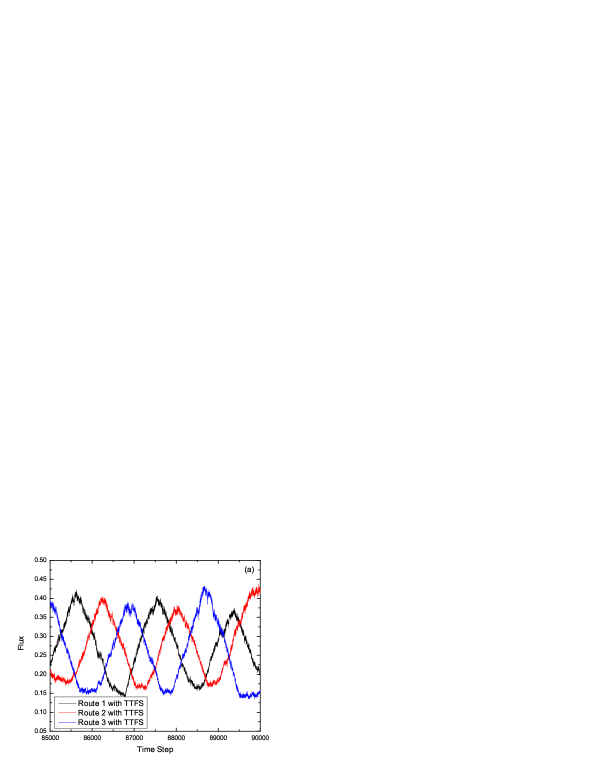
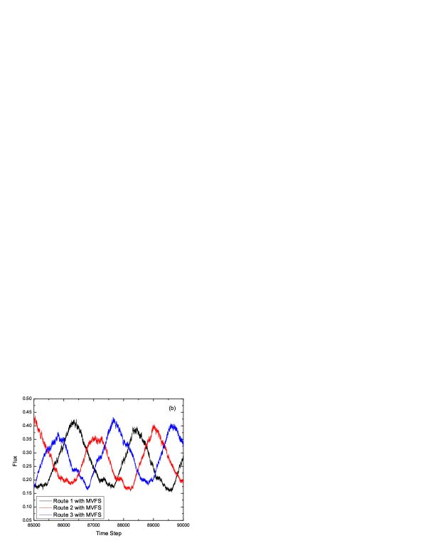
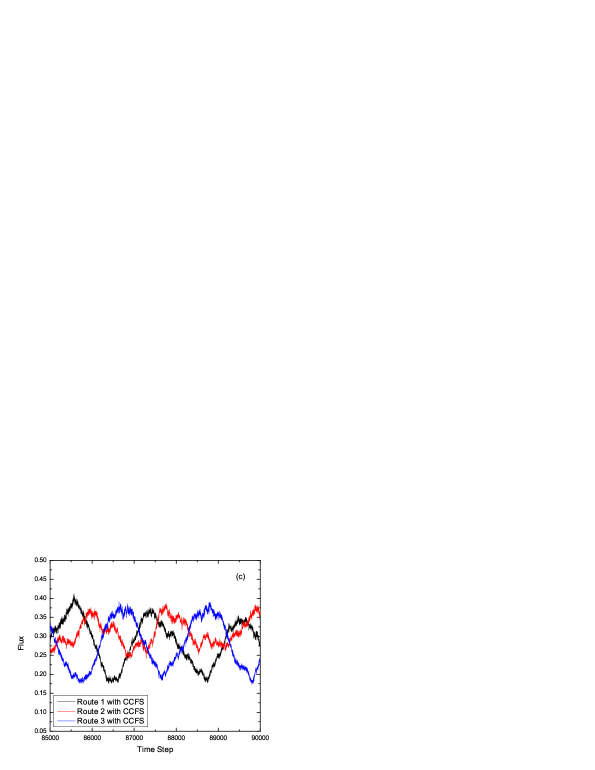
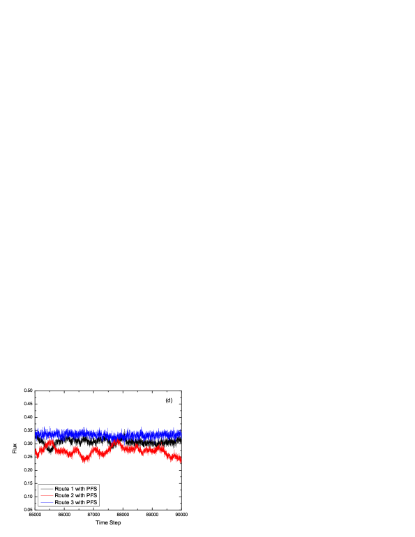
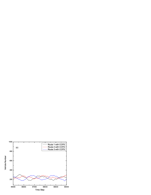
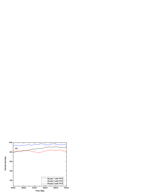
In Fig.4, vehicle number versus time step shows almost the same tendency as Fig.3, and that the routes’ accommodating capacity is greatly enhanced with an increase in average vehicle number from 230 to 870, so perhaps the high fluxes of three routes with PFS are mainly due to the increase of vehicle number. Here, someone may ask if the high vehicle number will result in the jammed cluster in each route. As to the routes’ stability, we know PFS is the best one (see Fig.3 and Fig.4), which means the vehicles should be almost uniformly distributed on each route instead of being together at the end of the routes. Furthermore, even there are 870 vehicles on each route, most vehicles can still occupy 2 sites on each lane and a few vehicles may even occupy 3 route sites because the total length of each route is fixed to be 2000 sites. Meanwhile, this means there is only one site between most of the vehicles. Though the vehicles are almost distributed separately on each lane, the one exit structure make jams still have a chance to happen at the end of the route, however, PFS can prevent jams from further expanding and alleviate the negative effects as much as possible, so that the jammed state will disappear soon. So as to analogize, even the jams happen again, the poor road condition will be relieved in a short time. Hence, there is some connection between the high accommodating capacity shown in Fig.4 and the traffic jams discussed in the paragraph above.

Figure 4: (Color online)(a) Vehicle number of each route with travel time feedback strategy. (b) Vehicle number of each route with mean velocity feedback strategy. (c) Vehicle number of each route with congestion coefficient feedback strategy. (d) Vehicle number of each route with prediction feedback strategy. The parameters are set the same as in Figure 3.

In Fig.5, speed versus time step shows that although the speed is the stablest by using prediction feedback strategy, it is the lowest among the four different strategies. The reason is that the speed partially depends on the number of empty sites between two vehicles on the lane. As mentioned before, the routes’ accommodating capacity is the best by using PFS, indicating the speed adopting PFS the lowest. From the stability of the velocity, we infer that the vehicles should drive at almost uniform speeds on each route. Without consider other factors, the speed should be a little more than one because there is only one site between most of the vehicles as mentioned above and the vehicle behind another vehicle can move at most the current empty sites between them which is also required by NS mechanism. If we take the random brake effects and the occasional jams at the end of the route into account, the vehicles’ average velocity low than one is possible and reasonable; therefore, the average velocity $V_{avg}\sim 0.7$ in this paper could be understood and there should be no conflicts between the average velocity and the almost uniform distribution of vehicles on each route. Other three strategies’ high speeds may result from the vehicles at the beginning or middle parts of the lane which have high velocities instead of the vehicles near the exit, because the average velocity in each lane depends on all vehicles’ velocities. Fortunately, flux consists of two parts, mean velocity and vehicle density. Therefore, as long as the vehicle number (because the vehicle density is $\rho$=N/L, and the L is fixed to be 2000, so $\rho$ $\propto$ vehicle number (N)) is large enough, the flux can also be the largest.

Figure 5: (Color online)(a) Average speed of each route with travel time feedback strategy. (b) Average speed of each route with mean velocity feedback strategy. (c) Average speed of each route with congestion coefficient feedback strategy. (d) Average speed of each route with prediction feedback strategy. The parameters are set the same as in Figure 3.

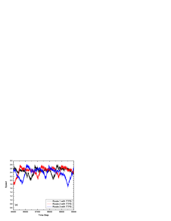
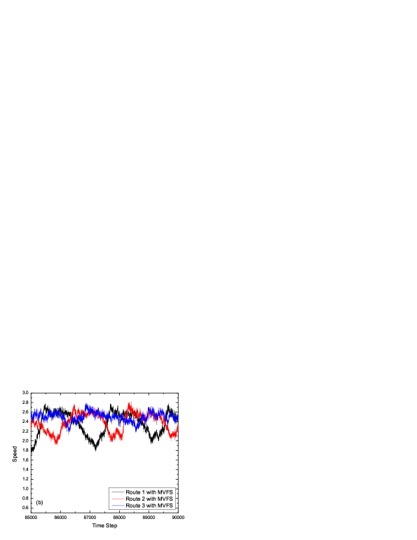
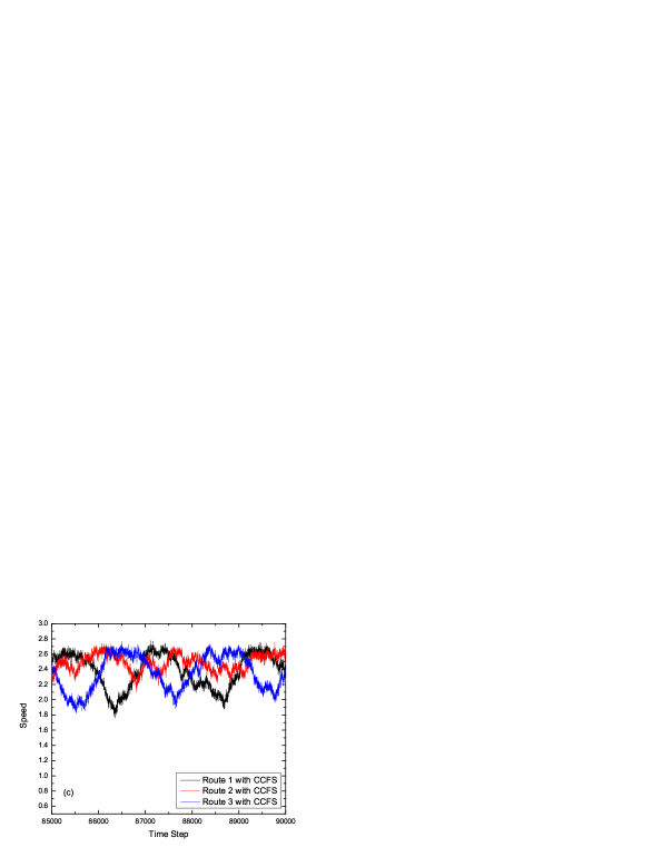
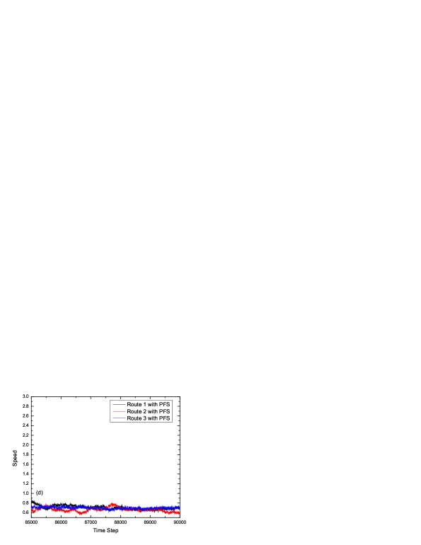
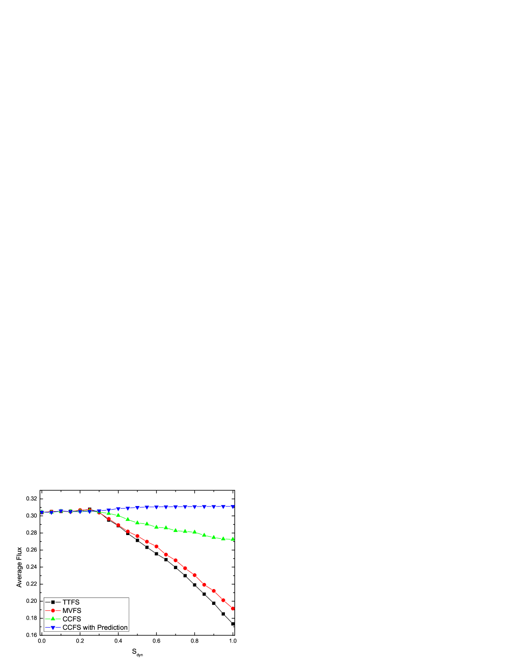
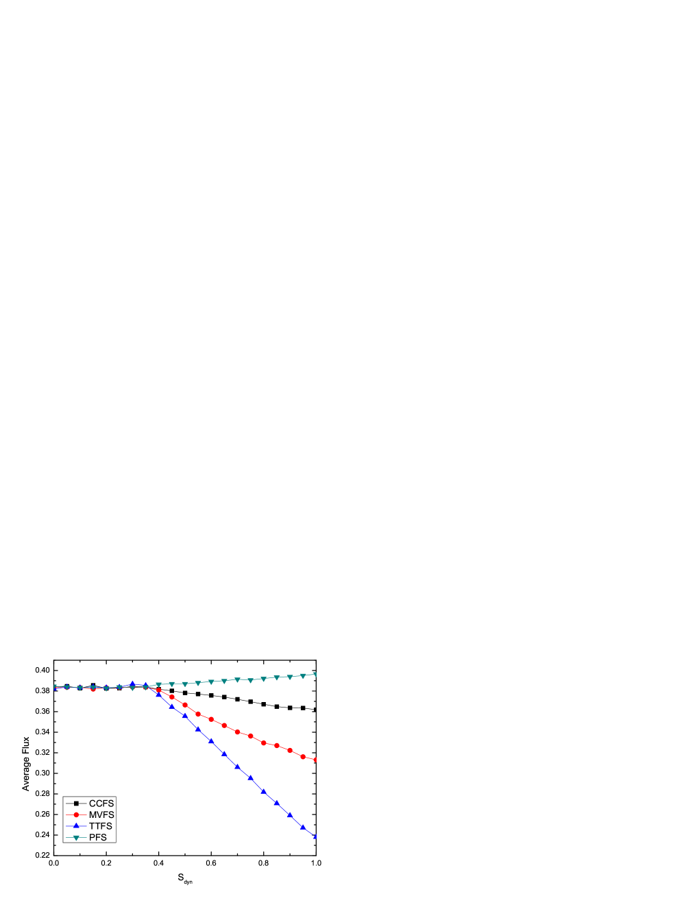
Fig.6 shows that the average flux fluctuates feebly with a persisting increase of dynamic travelers by using four different strategies. As to the routes’ processing capacity, the prediction feedback strategy is proved to be the best one because the flux is always the largest at each $\emph{S}_{dyn}$ value and enhances with a persisting increase of dynamic travelers. A question here for some readers is why the average fluxes in Fig.6 adopting four different strategies are smaller than that (see Fig.7) shown in the former work[23] where the traffic system has only two routes and the prediction time($\emph{T}_{p}$) is fixed to be 60. The reason is that the three-route system in this paper still permits at most one car to enter the entrance at each time step. Hence, more routes the traffic system owns, lower average fluxes it has.

Figure 6: (Color online) Average flux by performing different strategies vs $\emph{S}_{dyn}$ in the three-route system; L is fixed to be 2000, p is fixed to be 0.25 and $\emph{T}_{p}$ is fixed to be 260.

Figure 7: (Color online) Average flux by performing different strategies vs $\emph{S}_{dyn}$ in two-route system; L is fixed to be 2000, p is fixed to be 0.25 and $\emph{T}_{p}$ is fixed to be 60.

IV. CONCLUSION

We obtain the simulation results of applying four different feedback strategies, i.e., TTFS, MVFS, CCFS and PFS on a three-route scenario all with respect to flux, number of vehicles, speed, average flux versus $\emph{T}_{p}$ and average flux versus $\emph{S}_{dyn}$. The results indicate that PFS has more advantages than the other three strategies in the three-route system which has only one entrance and one exit. We also find out that it will take much more time to reach the stable state in the three-route system than that in the two-route system. In contrast with the other three feedback strategies, PFS can significantly improve the road condition, including increasing vehicle number and flux, reducing oscillation, and that average flux enhances with increase of $\emph{S}_{dyn}$. And it can be understood because PFS can eliminate the lag effect. The numerical simulations demonstrate that the prediction time ($\emph{T}_{p}$) plays a very important role in improving the road situation.

We also do the simulation of average flux versus $\emph{T}_{p}$ on a four-route scenario (see Fig.8) which is obtained by 90000 iterations excluding the initial 5000 time steps. We can see that in Fig.8 the prediction time ($\emph{T}_{p}$) corresponding to the highest value of the average flux is about 1020 time steps which are much longer than those in the two-route and three-route systems. Here ,we can make a reasonable assumption that one car passes the route with the average speed $v_{mean}$ $\sim$ 2, then the time it passes the route is $\emph{T}_{pass}$ $\sim$ 1000 because of the total length of one route L=2000. If $\emph{T}_{pass}$ and $\emph{T}_{p}$ are of the same order of magnitude($\emph{T}_{pass}$ $\sim$ $\emph{T}_{p}$), then the prediction feedback strategy will become invalid because the car at the entrance of the route at first will leave the traffic system after $\emph{T}_{pass}$. So we come to the conclusion that the prediction feedback strategy is appropriate in multi-route systems when the length of the route is long enough to ensure $\emph{T}_{pass}$ $>$ $\emph{T}_{p}$.

Figure 8: Average flux vs prediction time($\emph{T}_{p}$) in a four-route model. The parameters are L=2000, p=0.25, and $\emph{S}_{dyn}$=0.5.

Acknowledgments:

C.-F Dong would like to thank Dr. Nan Liu at the University of Chicago and the reviewers for some helpful comments while we were preparing the manuscript.

This work has been partially supported by the National Basic Research Program of China (973 Program No. 2006CB705500), the National Natural Science Foundation of China (Grant Nos. 60744003, 10635040,10532060), the Specialized Research Fund for the Doctoral Program of Higher Education of China (Grant No. 20060358065) and National Science Fund for Fostering Talents in Basic Science (J0630319).

References

- [1] D. Chowdhury, L. Santen and A. Schadschneider, Phys. Rep. 329, 199 (2000).
- [2] D. Helbing, Rev. Mod. Phys. 73, 1067 (2001).
- [3] T. Nagatani, Rep. Prog. Phys. 65, 1331 (2002).
- [4] R. W. Rothery, in Traffic Flow Theory, edited by N. Gartner, C. J. Messner, and A. J. Rathi, Transportation Research Board Special Report, Vol. 165 (Transportation Research Board, Washington, D.C., 1992), Chap. 4.
- [5] I. Prigogine and F. C. Andrews, Oper. Res. 8, 789 (1960).
- [6] S. L. Paveri-Fontana, Transp. Res. 9, 225 (1975).
- [7] H. Lehmann, Phys. Rev. E 54, 6058 (1996).
- [8] C. Wagner, C. Hoffmann, R. Sollacher, J. Wagenhuber, and B. Schürmann, Phys. Rev. E 54, 5073 (1996).
- [9] D. Helbing, Phys. Rev. E 53, 2366 (1996).
- [10] D. Helbing, Phys. Rev. E 57, 6176 (1998).
- [11] D. Helbing and M. Treiber, Phys. Rev. Lett. 81,3042(1998).
- [12] K. Nagel and M. Schreckenberg, J. Phys. I 2, 2221 (1992).
- [13] O. Biham, A. A. Middleton, and D. Levine, Phys. Rev. A 46, R6124 (1992).
- [14] Y. Yokoya, Phys. Rev. E 69, 016121 (2004).
- [15] T. L. Friesz, J. Luque, R. L. Tobin, and B.-W. Wie, Oper. Res. 37, 893 (1989).
- [16] M. Ben-Akiva, A. de Palma, and I. Kaysi, Transp. Res., PartA 25A, 251 (1991).
- [17] H. S. Mahmassani and R. Jayakrishnan, Transp. Res., Part A 25A, 293 (1991).
- [18] R. Arnott, A. de Palma, and R. Lindsey, Transp. Res., Part A 25A, 309 (1991).
- [19] P. Kachroo and K. Ozbay, Transp. Res. Rec. 1556, 137 (1996).
- [20] J. Wahle, A. L. C. Bazzan, F. Klügl, and M. Schreckenberg, Physica A 287, 669 (2000).
- [21] K. Lee, P.-M. Hui, B.-H. Wang, and N. F. Johnson, J. Phys. Soc. Jpn. 70, 3507 (2001).
- [22] W.-X. Wang, B.-H. Wang, W.-C. Zheng, C.-Y. Yin, and T. Zhou, Phys. Rev. E 72, 066702 (2005).
- [23] C.-F Dong, X. Ma, G.-W. Wang, X.-Y. Sun, and B.-H. Wang, Physica A 388, 4651 (2009).