The relation between and for solar-like oscillations
Abstract
Establishing relations between global stellar parameters and asteroseismic quantities can help improve our understanding of stellar astrophysics and facilitate the interpretation of observations. We present an observed relation between the large frequency separation, , and the frequency of maximum power, . We find that , allowing prediction of to about 15 per cent given . Our result is further supported by established scaling relations for and and by extended stellar model calculations, which confirm that can be estimated using this relation for basically any star showing solar-like oscillations in the investigated range (M).
keywords:
stars: fundamental parameters — stars: oscillations — stars: interiors.1 Introduction
Simple scaling relations for asteroseismic quantities have proven very useful when analysing stellar oscillations. In particular, relations for scaling the quantities (Brown et al., 1991) and (Ulrich, 1986) from the Sun have been widely used to constrain stellar global parameters, or simply to verify the asteroseismic signal of stars that already had well-constrained stellar parameters. Here, is the frequency of maximum power of the oscillations, and is the sol-called large frequency separation between consecutive overtones. For the Sun, Hz and Hz.
Over the past decade, detections of solar-like oscillations in other stars have been growing in number (see reviews by Aerts et al., 2008; Bedding & Kjeldsen, 2008), and the CoRoT space mission has caused a recent surge (Michel et al., 2008; de Ridder et al., 2009). This flow of data is expected to increase to a flood with the Kepler mission (Christensen-Dalsgaard et al., 2008). For many stars, knowing or can help constrain the stellar parameters considerably (Stello et al., 2008; Kallinger et al., 2008; Stello et al., 2009; Miglio et al., 2009) and hence yield important new insights into stellar structure and evolution, even without a full asteroseismic analysis. In addition, recent developments of automated software for asteroseismic data analysis benefit from knowing a simple relation between and (Mathur et al., 2009; Huber et al., 2009; Hekker et al., 2009b).
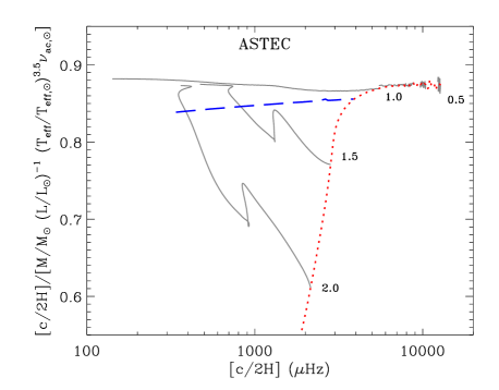
In this Letter we investigate the relation between and , building on previous studies to show how these two quantities are related to each other and to the global stellar parameters. We also carry out stellar model calculations to support this investigation, including a comparison of stellar models with the established scaling relations for and .
2 The observed relation
Table 1 shows published measurements of and for 55 stars including the Sun. In some cases, where the value of was not specified, we have estimated it from the published power spectra. The location of the stars in the – diagram are shown in Fig. 1.
| Star | Source | ||
| (Hz) | (Hz) | ||
| Cet | 170 | 4500 | Teixeira et al. (2009) |
| Cen B | 161.4 | 4100 | Kjeldsen et al. (2008) |
| Sun | 134.8 | 3100 | Kjeldsen et al. (2008) |
| Hor | 120 | 2700 | Vauclair et al. (2008) |
| Pav | 120.3 | 2600 | Mosser et al. (2008) |
| Cen A | 106.2 | 2400 | Kjeldsen et al. (2008) |
| HD175726 | 97 | 2000 | Garcia et al. (2009) |
| Ara | 90 | 2000 | Bouchy et al. (2005) |
| HD181906 | 87.5 | 1900 | Garcia et al. (2009) |
| HD49933 | 85.9 | 1760 | Garcia et al. (2009) |
| HD181420 | 75 | 1500 | Garcia et al. (2009) |
| Vir | 72 | 1400 | Carrier et al. (2005b) |
| Her | 56.5 | 1200 | Bonanno et al. (2008) |
| Hyi | 57.5 | 1000 | Kjeldsen et al. (2008) |
| Procyon | 55 | 1000 | Arentoft et al. (2008) |
| Boo | 39.9 | 750 | Carrier et al. (2005a) |
| Ind | 25.1 | 320 | Kjeldsen et al. (2008) |
| Ser | 7.7 | 130 | Barban et al. (2004) |
| Hya | 6.8 | 90 | Frandsen et al. (2002) |
| Vol | 4.9 | 51 | unpublished WIRE data |
| Oph | 5.3 | 50 | Barban et al. (2007) |
| Dra | 4.0 | 36 | unpublished WIRE data |
| Oph | 4.5 | 35 | unpublished WIRE data |
| HR3280 | 3.2 | 25 | unpublished WIRE data |
| 31 CoRoT giants | 2–7 | 15–73 | Kallinger et al. (2008) |


In Fig. 2 we plot versus for the data listed in Table 1. We see a remarkably tight relation over nearly three orders of magnitude. A power-law fit gives
| (1) |
The two stars that deviate the most from this relation are Ser and Hya. In both cases, there are reported ambiguities in the determination of the large separation, which could explain the deviation. Apart from those two cases, all stars in Fig. 2 fall within per cent and per cent of the fitted relation, while the main sequence stars alone fall within per cent. We note that Hekker et al. (2009b) have confirmed the tight correlation for a sample of several hundred red giants observed by CoRoT, which also seems to indicate a tendency for some stars to fall below the relation.
3 Scaling relations
Can previously published scaling relations for and explain the observed relation between them? It is well-established (e.g. Ulrich, 1986) that, to a good approximation, is proportional to the square root of the stellar density:
| (2) |
Also, following Brown et al. (1991) and Kjeldsen & Bedding (1995), we expect to scale as the acoustic cut-off frequency, . Hence,
| (3) |
where it is observed for the Sun that (Balmforth & Gough, 1990; Fossat et al., 1992). Given that and scale differently with stellar parameters, the tightness of the correlation in Fig. 2 is perhaps surprising. To understand this, we raise Eq. (3) to the power and divide by Eq. (2) which, after rearranging, gives
| (4) |
The tight relation in Fig. 2 leads us to conclude that the scaling factor in square brackets in Eq. (4) must be approximately constant when . Indeed, this is easy to see because that value of eliminates almost completely the parameter that varies the most over the stars being considered, namely , and leaves a very weak dependence on and . This is illustrated in Fig. 3, which shows the scaling factor for the observed value . The scaling factor indeed covers a band 25 per cent wide for the region sampled by the stars (see Fig. 1), in agreement with the to per cent deviation shown by the observational data in Fig. 2. Figure 3 further supports the lower scatter observed for the main sequence stars and the higher, slightly skewed, scatter for red giants.
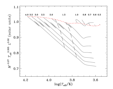
We have determined the value of that minimizes the spread in the scaling factor and found that it depends slightly on the stellar parameter range that we consider. For example, consideration of the entire model grid requires , while considering only ZAMS models gives .
4 Models
We now expand our investigation of the – relation using two sets of stellar models. One is a dense grid, comprising over a million models derived using the Aarhus stellar evolution code astec (Christensen-Dalsgaard, 2008b) and the adiabatic pulsation code adipls (Christensen-Dalsgaard, 2008a). This grid is slightly expanded in parameter space but otherwise identical to the one constructed by Stello et al. (2009) (see references herein). The other is a set derived using the Yale code yrec (Demarque et al., 2008) with mixing-length parameter , initial hydrogen abundance , and metallicity . Although the set of yrec models is more sparse, with a total of 92 models, it spans almost uniformly the same range in parameter space as the astec grid. The region covered by the models is indicated by the evolutionary tracks in Fig. 1.
In addition to the global stellar parameters , , and , we calculated for each model the large frequency separation as the inverse of the sound travel time through the star:
| (5) |
where is the sound speed (Tassoul, 1980; Gough, 1986). We also calculated the acoustic cutoff frequency by assuming an isothermal atmosphere, which gives (Balmforth & Gough, 1990)
| (6) |
evaluated at the surface ( ). Here, is the density scale height, is pressure, is gravity, and is density.

In Fig. 4 we show a subset of the astec grid for a fixed metallicity (). Contours of constant (magenta) are almost parallel to contours of constant (cyan), indicating a strong correlation. Hence, knowing one of these two quantities gives a good estimate of the other. This is particularly pronounced in the lower-right corner of the diagram, corresponding to cool main-sequence and subgiant stars. A somewhat weaker correlation is seen in the red giant phase. Note that we neglected the post He-core burning phase, including any mass loss associated with red giant branch evolution. If included, it would blur the contours in this region (Stello et al., 2008).
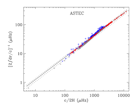
Figure 5 shows the relation between and for the astec models. We find very similar results for the yrec models. Stars hotter than the red edge of the instability strip are generally not expected to exhibit solar-like oscillations and are shown in blue, while cool models are shown in red and grey. We compare the models with observations by fitting a power law with the observed value of fixed. We see excellent agreement with observations, particularly at low masses (M⊙, red), which is perhaps not surprising since the observations are predominantly from low-mass stars. Interestingly, all cool main-sequence models – high values of – show a very tight relation, while for more evolved models – lower values of – the higher mass ones (grey) scatter more and fall below the power-law relation. This agrees with the observations and with the scaling factor in Eq. (4) (see also Fig. 3). Finally, we found that the theoretical – relation was not notably sensitive to metallicity. However, it remains to be explained why , which depends on the stellar mean density, correlates so strongly with , which depends on the local conditions in the atmosphere.
5 Discussion
Several points should be kept in mind when comparing the model calculations with the observations. Firstly, we do not measure directly in stars and instead rely on its relation to (see Eq. 3), assuming that / does not vary from the solar value. In addition, can be difficult to define and measure, especially for stars with broad or double-humped envelopes, as seen in Procyon (Bedding & Kjeldsen, 2006; Arentoft et al., 2008). On the other hand, varies with frequency and mode degree, and its measurement from the power spectrum gives an average that will not be exactly equal to . That said, Fig. 5 clearly supports the tight – relation that we observe.
The preceding comments relate to measuring and from observations. We should also consider the various ways in which these quantities can be estimated from the models. So far we have used Eqs. (5) and (6). Here, we derive the large frequency separation and the acoustic cutoff frequency from the models in other ways and investigate any significant systematic differences. The large separation was derived by fitting to 11 consecutive radial orders around , which we denote fit. The result for the yrec models (Fig. 6, left panel) shows agreement within a few per cent between and fit, although we note that the ratio fit is always higher than unity. We see similar results for the astec models.
We then tested two additional ways to calculate the acoustic cutoff frequency. Firstly, was derived from the actual density gradient in the model, but still using Eq. (6). Secondly we used the full expression (Balmforth & Gough, 1990).
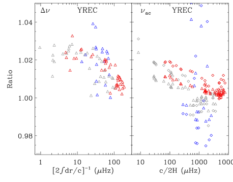
The results are shown in Fig. 6 (right panel). Apart from a few hot models that deviate by up to 25 per cent, the agreement is again within a few per cent. For our purpose of investigating the relation between and , a few per cent difference in either quantity is not important, but they should be kept in mind for other applications.
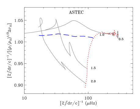
Finally, it is interesting to investigate how well the scaling relations for and (Eqs. 2 and 3) agree with the model calculations (Eqs. 5 and 6). Figure 7 examines how well scales with . For cool models the agreement is particularly good, almost independent of the evolutionary state, while it deteriorates slightly for hot models (those below the blue line). However, we note that systematically overestimates the large frequency separation for cool models, corresponding to 2–3 per cent for the Sun.
In a similar way Fig. 8 shows that the model calculations of follow the scaling from the Sun quite well. The ratio is always below unity because we evaluate at the surface defined as , where is slightly below its maximum value, which occurs further out in the atmosphere. As with , we conclude that the best agreement is for the cool models. We find similar results for the yrec models.
6 Conclusions
This Letter points out that the ratio / varies very weakly with stellar parameters, so that it is essentially constant. Hence, if either one of these parameters is measured, this gives a very useful and robust estimate of the other without any prior knowledge of the stellar global parameters, , , , and . We anticipate this relation can be used to establish the most plausible large separation in case of ambiguity for datasets where can be determined. This has already been implemented for automated analysis of Kepler data (Hekker et al., 2009a; Huber et al., 2009; Mathur et al., 2009). In addition, we showed that the well-used scaling relations for and agree within a few per cent with stellar model calculations for cool models ( K), from the main sequence to the red giant branch, with a slightly increasing deviation for hotter models.
Acknowledgments
DS acknowledge support from the Australian Research Council. WJC and YE acknowledge the support of the UK Science and Technology Facilities Council (STFC). DS would like to thank Douglas Gough for fruitful discussions.
References
- Aerts et al. (2008) Aerts, C., Christensen-Dalsgaard, J., Cunha, M., & Kurtz, D. W. 2008, Sol. Phys., 251, 3
- Arentoft et al. (2008) Arentoft, T., Kjeldsen, H., Bedding, T. R., et al. 2008, ApJ, 687, 1180
- Balmforth & Gough (1990) Balmforth, N. J. & Gough, D. O. 1990, ApJ, 362, 256
- Barban et al. (2004) Barban, C., De Ridder, J., Mazumdar, A., et al. 2004, in Proceedings of the SOHO 14 / GONG 2004 Workshop (ESA SP-559). ”Helio- and Asteroseismology: Towards a Golden Future”. 12-16 July, 2004. New Haven, Connecticut, USA. Editor: D. Danesy., 113
- Barban et al. (2007) Barban, C., Matthews, J. M., de Ridder, J., et al. 2007, A&A, 468, 1033
- Bedding & Kjeldsen (2006) Bedding, T. R. & Kjeldsen, H. 2006, Memorie della Societa Astronomica Italiana, 77, 384
- Bedding & Kjeldsen (2008) Bedding, T. R. & Kjeldsen, H. 2008, in Astronomical Society of the Pacific Conference Series, Vol. 384, 14th Cambridge Workshop on Cool Stars, Stellar Systems, and the Sun, ed. G. van Belle, 21
- Bonanno et al. (2008) Bonanno, A., Benatti, S., Claudi, R., et al. 2008, ApJ, 676, 1248
- Bouchy et al. (2005) Bouchy, F., Bazot, M., Santos, N. C., Vauclair, S., & Sosnowska, D. 2005, A&A, 440, 609
- Brown et al. (1991) Brown, T. M., Gilliland, R. L., Noyes, R. W., & Ramsey, L. W. 1991, ApJ, 368, 599
- Carrier et al. (2005a) Carrier, F., Eggenberger, P., & Bouchy, F. 2005a, A&A, 434, 1085
- Carrier et al. (2005b) Carrier, F., Eggenberger, P., D’Alessandro, A., & Weber, L. 2005b, New Astronomy, 10, 315
- Christensen-Dalsgaard (2008a) Christensen-Dalsgaard, J. 2008a, Ap&SS, 316, 113
- Christensen-Dalsgaard (2008b) Christensen-Dalsgaard, J. 2008b, Ap&SS, 316, 13
- Christensen-Dalsgaard et al. (2008) Christensen-Dalsgaard, J., Arentoft, T., Brown, T. M., et al. 2008, Communications in Asteroseismology, 157, 266
- de Ridder et al. (2009) de Ridder, J., Barban, C., Baudin, F., et al. 2009, Nature, 459, 398
- Demarque et al. (2008) Demarque, P., Guenther, D. B., Li, L. H., Mazumdar, A., & Straka, C. W. 2008, Ap&SS, 316, 31
- Fossat et al. (1992) Fossat, E., Regulo, C., Roca Cortes, T., et al. 1992, A&A, 266, 532
- Frandsen et al. (2002) Frandsen, S., Carrier, F., Aerts, C., et al. 2002, A&A, 394, L5
- Garcia et al. (2009) Garcia, R. A., Regulo, C., Samadi, R., et al. 2009, preprint (astro-ph/0907.0608)
- Gough (1986) Gough, D. O. 1986, in Hydrodynamic and Magnetodynamic Problems in the Sun and Stars, ed. Y. Osaki, 117
- Hekker et al. (2009a) Hekker, S., Broomhall, A.-M., Chaplin, W. J., et al. 2009a, submitted to MNRAS
- Hekker et al. (2009b) Hekker, S., Kallinger, T., Baudin, F., et al. 2009b, preprint (astro-ph/0906.5002)
- Huber et al. (2009) Huber, D., Stello, D., Bedding, T. R., et al. 2009, submitted to Communication in Asteroseismology
- Kallinger et al. (2008) Kallinger, T., Weiss, W. W., Barban, C., et al. 2008, preprint (astro-ph/0811.4674)
- Kjeldsen & Bedding (1995) Kjeldsen, H. & Bedding, T. R. 1995, A&A, 293, 87
- Kjeldsen et al. (2008) Kjeldsen, H., Bedding, T. R., Arentoft, T., et al. 2008, ApJ, 682, 1370
- Mathur et al. (2009) Mathur, S., Garcia, R. A., Regulo, C., et al. 2009, preprint (astro-ph/0907.1139)
- Michel et al. (2008) Michel, E., Baglin, A., Auvergne, M., et al. 2008, Science, 322, 558
- Miglio et al. (2009) Miglio, A., Montalban, J., Baudin, F., et al. 2009, A&A, 503, L21
- Mosser et al. (2008) Mosser, B., Deheuvels, S., Michel, E., et al. 2008, A&A, 488, 635
- Saio & Gautschy (1998) Saio, H. & Gautschy, A. 1998, ApJ, 498, 360
- Stello et al. (2008) Stello, D., Bruntt, H., Preston, H., & Buzasi, D. 2008, ApJ, 674, L53
- Stello et al. (2009) Stello, D., Chaplin, W. J., Bruntt, H., et al. 2009, ApJ, 700, 1589
- Tassoul (1980) Tassoul, M. 1980, ApJS, 43, 469
- Teixeira et al. (2009) Teixeira, T. C., Kjeldsen, H., Bedding, T. R., et al. 2009, A&A, 494, 237
- Ulrich (1986) Ulrich, R. K. 1986, ApJ, 306, L37
- Vauclair et al. (2008) Vauclair, S., Laymand, M., Bouchy, F., et al. 2008, A&A, 482, L5