Abstract

Total Internal Reflection Microscopy (TIRM) is a sensitive non-invasive technique to measure the interaction potentials between a colloidal particle and a wall with femtonewton resolution. The equilibrium distribution of the particle-wall separation distance $z$ is sampled monitoring the intensity $I$ scattered by the Brownian particle under evanescent illumination. Central to the data analysis is the knowledge of the relation between $I$ and the corresponding $z$, which typically must be known a priori. This poses considerable constraints to the experimental conditions where TIRM can be applied (short penetration depth of the evanescent wave, transparent surfaces). Here, we introduce a method to experimentally determine $I(z)$ by relying only on the distance-dependent particle-wall hydrodynamic interactions. We demonstrate that this method largely extends the range of conditions accessible with TIRM, and even allows measurements on highly reflecting gold surfaces where multiple reflections lead to a complex $I(z)$.

OCIS codes: (120.0120) Instrumentation, measurement, and metrology; (120.5820) Scattering measurements; (180.0180) Microscopy; (260.6970) Total internal reflection; (240.0240) Optics at surfaces; (240.6690) Surface waves.

1 Introduction

Total Internal Reflection Microscopy (TIRM) [1, 2] is a fairly new technique to optically measure the interactions between a single colloidal particle and a surface using evanescent light scattering. The distribution of the separation distances sampled by the particle’s Brownian motion is used to obtain the potential energy profile $U(z)$ of the particle-surface interactions with sub-$k_{B}T$ resolution, where $k_{B}T$ is the thermal energy. Amongst various techniques available to probe the mechanical properties of microsystems, the strength of TIRM lies in its sensitivity to very weak interactions. Atomic Force Microscopy (AFM) [3, 4] requires a macroscopic cantilever as a probe and is typically limited to forces down to several piconewton ($10^{-12}\,N$); the sensitivity of Photonic Force Microscopy (PFM) [5, 6, 7] can even reach a few femtonewtons ($10^{-15}\,N$), but this method is usually applied to bulk measurements far from any surface. TIRM, instead, can measure forces with femtonewton resolution acting on a particle near a surface. Over the last years, TIRM has been successfully applied to study electrostatic [8, 9], van der Waals [10], depletion [11, 12, 13, 14], magnetic [15], and, rather recently, critical Casimir [16] forces.

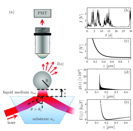
Fig. 1: Total Internal Reflection Microscopy (TIRM). (a) Schematic of a typical TIRM setup: a Brownian particle moves in the evanescent electromagnetic field generated by total internal reflection of a laser beam; its scattering is collected by an objective lens; and the scattering intensity is recorded using a photomultiplier (PMT). (b) Typical experimental scattering intensity time-series (polystyrene particle in water, $R=1.45\,\mu m$). (c) Exponential intensity-distance relation ($\beta=120\,nm$). (d) Particle position distribution (acquisition time $1200\,s$, sampling rate $500\,Hz$). (e) Experimental (dots) and theoretical (line) potential obtained from the position distribution using the Boltzmann factor.

A schematic sketch of a typical TIRM setup is presented in Fig. 1(a). To track the Brownian trajectory of a spherical colloidal particle diffusing near a wall, an evanescent field is created at the substrate-liquid interface. The scattered light is collected with a microscope objective and recorded with a photomultiplier connected to a data acquisition system. Fig. 1(b) shows a typical example of an experimentally measured intensity time-series $I_{t}$ of a polystyrene particle with radius $R=1.45\,\mu m$ in water.

Due to the evanescent illumination, the intensity of the light scattered by the particle is quite sensitive to the particle-wall distance. If the corresponding intensity-distance relation $I(z)$ is known (and monotonic), the vertical component of the particles trajectory $z_{t}$ can be deduced from $I_{t}$. To obtain $I(z)$, it is in principle required to solve a rather complex Mie scattering problem, i.e. the scattering of a micron-sized colloidal particle under evanescent illumination close to a surface [17, 18], where multiple reflections between the particle and the substrate and Mie resonances must be accounted for [19, 20, 21, 22]. When such effects can be neglected, the scattering intensity is proportional to the evanescent field intensity and, since the latter decays exponentially, TIRM data are typically analyzed using a purely exponential $I(z)=I_{0}e^{-z/\beta}$ [1, 2, 17, 18, 23] (Fig. 1(c)), where $\beta=\lambda/4\pi\sqrt{n_{s}^{2}\sin^{2}\theta-n_{m}^{2}}$ is the evanescent field penetration depth, $\lambda$ the incident light wavelength, $n_{s}$ the substrate refractive index, $n_{m}$ the liquid medium refractive index, and $\theta$ the incidence angle, which must be larger than the critical angle $\theta_{c}=\arcsin(n_{m}/n_{s})$. $I_{0}$ is the scattering intensity at the wall, which can be determined e.g. using a hydrodynamic method proposed [24].

From the obtained $z_{t}$ the particle-wall interaction potential, i.e. $U(z)$, is easily derived by applying the Boltzmann factor $U(z)=-k_{B}T\ln{p(z)}$ to the calculated position distribution $p(z)$ (Fig. 1(d,e)). For an electrically charged dielectric particle suspended in a solvent, the interaction potential typically corresponds to $U(z)=B\exp{(-\kappa z)}+[\frac{4}{3}\pi R^{3}(\rho_{p}-\rho_{m})g-F_{s}]z$. The first term is due to double layer forces with $\kappa^{-1}$ the Debye length and $B$ a prefactor depending on the surface charge densities of the particle and the wall [1, 2, 9]. The second term describes the effective gravitational contributions with $\rho_{p}$ and $\rho_{m}$ the particle and solvent density and $g$ the gravitational acceleration constant; $F_{s}$ takes into account additional optical forces, which may result from a vertically incident laser beam often employed as a two-dimensional optical trap to reduce the lateral motion of the particle [25]. Depending on the experimental conditions, additional interactions, such as depletion or van der Waals forces, may arise.

Despite the broad range of phenomena that have successfully been addressed with TIRM, most studies have been carried out with small penetration depths (at most $\beta\approx 100\,nm$), and have therefore been limited to rather small particle-substrate distances $z$. In addition, no TIRM studies on highly reflecting walls, e.g. gold surfaces, have been reported, although such surfaces are interesting since they can support surface plasmons enhancing the evanescent field [26] and the optical near-field radiation forces [27, 28, 29]. Furthermore, gold coatings can be easily functionalized [30], which would allow to apply TIRM to e.g. biological systems. The reason for these limitations is the aforementioned problem to obtain a reliable $I(z)$ relationship under these conditions. For example, it has been demonstrated that large penetration depths (e.g. above $\approx 200\,nm$ in Ref. [31]) increase the multiple optical reflections between the particle and the wall, which in turn leads to a non-exponential $I(z)$ [21, 31]. Experiments combining TIRM and AFM found deviations from simple exponential behaviour very close to the wall even for shorter penetration depths [32]. In principle, such effects can be included into elaborate scattering models, however, this requires precise knowledge of the system properties and, in particular, of the refractive indices of particle, wall, and liquid medium [31]. Since the latter are prone to significant uncertainties (in particular for the colloidal particles), the application of TIRM under such conditions remains inaccurate.

Here, we introduce a method to experimentally determine $I(z)$ by making solely use of the experimentally acquired $I_{t}$ and of the distance-dependent hydrodynamic interactions between the particle and the wall. In particular, no knowledge about the shape of the potential $U(z)$ is required. We demonstrate the capability of this method by experiments and simulations, and we also apply it to experimental conditions with long penetration depths ($\beta=720\,nm$) and even with highly reflective gold surfaces.

2 Theory

2.1 Diffusion coefficient and skewness of Brownian motion near a wall

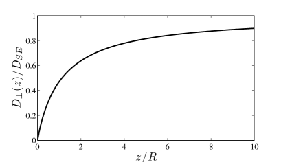
Fig. 2: Vertical diffusion coefficient $D_{\bot}(z)$ near a wall (Eq. (1)).

Colloidal particles immersed in a solvent undergo Brownian motion due to collisions with solvent molecules. This erratic motion leads to particle diffusion with the Stokes-Einstein diffusion coefficient $D_{SE}=k_{B}T/6\pi\eta R$, where $\eta$ is the shear viscosity of the liquid. It is well known that this bulk diffusion coefficient decreases close to a wall due to hydrodynamic interactions. From the solution of the creeping flow equations for a spherical particle in motion near a wall assuming nonslip boundary conditions and negligible inertial effects, one obtains for the diffusion coefficient in the vertical direction [33],

$$D_{\bot}(z)=\frac{D_{SE}}{l(z)}\mbox{,}$$ (1)

where $l(z)=\frac{4}{3}\sinh{\left(\alpha(z)\right)}\sum_{n=1}^{\infty}\frac{n(n+1)}{(2n-1)(2n+3)}\left[\frac{2\sinh{\left((2n+1)\alpha(z)\right)}+(2n+1)\sinh{\left(2\alpha(z)\right)}}{4\sinh^{2}{\left((n+0.5)\alpha(z)\right)}-(2n+1)^{2}\sinh^{2}{\left(\alpha(z)\right)}}-1\right]$ and $\alpha(z)=\cosh^{-1}\left(1+\frac{z}{R}\right)$. As shown in Fig. 2, $D_{\bot}$ first increases with $z$ approaching the corresponding bulk value at a distance of several particle radii away from the wall.

Experimentally, the diffusion coefficient can be obtained from the mean square displacement (MSD) calculated from a particle trajectory. For the $z$-component this reads ${\langle(z_{t+\Delta t}-z_{t})^{2}\rangle}=2D_{SE}\Delta t$, where $\langle...\rangle$ indicates average over time $t$. To account for a $z$-dependent diffusion coefficient close to a wall, one has to calculate the conditional MSD given that the particle is at time $t$ at position $z$, i.e. $\langle(z_{t+\Delta t}-z_{t})^{2}\mid z_{t}=z\rangle=2D_{\bot}(z)\Delta t$ where the equality is valid for $\Delta t\rightarrow 0$; in such limit, this expression is only determined by the particle diffusion even if the particle is exposed to an external potential $U(z)$. From this follows that $D_{\bot}(z)$ can be directly obtained from the particle’s trajectory

$$D_{\bot}(z)=\lim_{\Delta t\rightarrow 0}\frac{1}{2\Delta t}\left\langle(z_{t+\Delta t}-z_{t})^{2}\mid z_{t}=z\right\rangle\mbox{.}$$ (2)

Eq. (2) was employed already by several groups [34, 35] to validate Eq. (1).

The distribution of particle displacements $h(z;z_{0},\Delta t)$ around a given distance $z_{0}$ converges to a gaussian for $\Delta t\rightarrow 0$ and therefore its skewness – i.e. the normalized third central moment – converges to zero. Accordingly,

$$S(z)\equiv\lim_{\Delta t\rightarrow 0}\frac{1}{\Delta t^{2}}\left\langle\left(\frac{z_{t+\Delta t}-z_{t}-M(z,\Delta t)}{\sqrt{2D_{\bot}(z)}}\right)^{3}\mid z_{t}=z\right\rangle=0\mbox{,}$$ (3)

where $M(z,\Delta t)=\langle z_{t+\Delta t}-z_{t}\mid z_{t}=z\rangle=\underset{\hat{z}}{\arg\max}\;h(\hat{z};z,\Delta t)$, where $\underset{\hat{z}}{\arg\max}$ indicates the argument that maximize the given function.

2.2 Mean square displacement and skewness of the scattering intensity

In a TIRM experiment, $h(z;z_{0},\Delta t)$ is translated into a corresponding intensity distribution $h(I;I_{0},\Delta t)$ around intensity $I_{0}=I(z_{0})$, whose shape strongly depends on $I(z)$. In Fig. 3 we demonstrate how a particle displacement distribution $h(z;z_{0},\Delta t)$, which is gaussian for small $\Delta t$, translates into the corresponding scattered intensity distribution $h(I;I_{0},\Delta t)$ for an arbitrary non-exponential $I(z)$ dependence. In the linear regions of $I(z)$, the corresponding $h(I;I_{0},\Delta t)$ are also gaussian with the half-width determined by the slope of the $I(z)$ curve. In the non-linear part of $I(z)$, however, a non-gaussian intensity histogram with finite skewness is obtained.

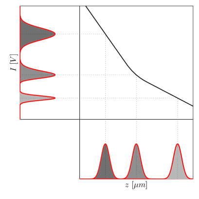
Fig. 3: Relation between position distributions and intensity distributions. Brownian diffusion of a particle around a point is symmetric, leading for small $\Delta t$ to a gaussian distribution $h(z;z_{0},\Delta t)$ (bottom). According to $I(z)$ this leads to the scattered intensity histograms $h(I;I_{0},\Delta t)$ (left): in the linear region of $I(z)$, $h(I;I_{0},\Delta t)$ is also gaussian with the width depending on $I^{\prime}$ (Eq. (4)); in the nonlinear region of $I(z)$ (central histogram), $h(I;I_{0},\Delta t)$ deviates from a gaussian and has a finite skewness depending on $I^{\prime\prime}$ (Eq. (5)).

In the following we calculate the MSD and the skewness of $h(I;I_{0},\Delta t)$ for an arbitrary $I(z)$, which we assume to be a continuous function with well defined first and second derivates $I^{\prime}$ and $I^{\prime\prime}$. In the vicinity of $z_{0}$, $I(z)$ can be therefore expanded in a Taylor series $I(z)=I(z_{0})+I^{\prime}(z_{0})(z-z_{0})+\frac{1}{2}I^{\prime\prime}(z_{0})(z-z_{0})^{2}$ for $z\rightarrow z_{0}$, where $I^{\prime}=\frac{dI}{dz}$ and $I^{\prime\prime}=\frac{d^{2}I}{dz^{2}}$. The MSD of $h(I;I_{0},\Delta t)$ is

$$\mathrm{MSD}(I)\equiv\lim_{\Delta t\rightarrow 0}\frac{1}{\Delta t}\left\langle(I_{t+\Delta t}-I_{t})^{2}\mid I_{t}=I\right\rangle=I^{\prime 2}(z)\cdot 2D_{\bot}(z)\mbox{,}$$ (4)

where $\left\langle(I_{t+\Delta t}-I_{t})^{2}\mid I_{t}=I\right\rangle=I^{\prime 2}\left\langle(z_{t+\Delta t}-z_{t})^{2}\mid I_{t}=I\right\rangle$ for $\Delta t\rightarrow 0$ and Eq. (2) has been used. The skewness of $h(I;I_{0},\Delta t)$ is

$$\mathrm{S}(I)\equiv\lim_{\Delta t\rightarrow 0}\frac{1}{\Delta t^{2}}\left\langle\left(\frac{I_{t+\Delta t}-I_{t}-M(I,\Delta t)}{\sqrt{\mathrm{MSD}(I)}}\right)^{3}\mid I_{t}=I\right\rangle=\frac{9}{2}\frac{I^{\prime\prime}(z)}{|I^{\prime}(z)|}\cdot\sqrt{2D_{\bot}(z)}\mbox{,}$$ (5)

with $M(I,\Delta t)=\underset{\hat{I}}{\arg\max}\;h(\hat{I};I,\Delta t)$ and $\left\langle(I_{t+\Delta t}-I_{t}-M(I,\Delta t))^{3}\mid I_{t}=I\right\rangle=I^{\prime 3}\left\langle(z_{t+\Delta t}-z_{t}-M(z,\Delta t))^{3}\mid z_{t}=z\right\rangle+\frac{3}{2}I^{\prime 2}I^{\prime\prime}\left\langle(z_{t+\Delta t}-z_{t}-M(z,\Delta t))^{4}\mid z_{t}=z\right\rangle$ for $\Delta t\rightarrow 0$ where the first term is null because of Eq. (3), and the second term is calculated using the properties of the momenta of a gaussian distribution $\left\langle(...)^{4}\right\rangle=3\left\langle(...)^{2}\right\rangle^{2}$.

In Fig. 4 we applied Eqs. (4) and (5) to the intensity time-series corresponding to a particle trajectory simulated using a Langevin difference equation assuming various $I(z)$ (Fig. 4(a,c,e)). The solid lines in Fig. 4(b,d,f) show the theoretical $\mathrm{MSD}(I)$ (black) and $\mathrm{S}(I)$ (red) and the dots the ones obtained from the simulations. When $I(z)$ is linear (Fig. 4(a)), $\mathrm{MSD}(I)$ is proportional to Eq. (1) and $\mathrm{S}(I)$ vanishes (Fig. 4(b)). When $I(z)$ is exponential (Fig. 4(c)) or a sinusoidally modulated exponential (Fig. 4(e), $\mathrm{MSD}(I)$ is not proportional to Eq. (1) and large values of the skewness occur as shown in (Figs. 4(d,f)). Small deviations between the theoretical curves and the numerical data can be observed for intensities where the particle drift becomes large in comparison to the time-step ($\Delta t=2\,ms$); in our case this corresponds to a slope of the potential of about $1\,pN/\mu m$, which is close to the upper force limit of typical TIRM measurements. If necessary such deviations can be reduced employing shorter time-steps.

Fig. 4: Various intensity-distance relations and their effect on $\mathrm{MSD}(I)$ (black) and skewness $\mathrm{S}(I)$ (red). Both theoretical values (solid lines) and the results from the analysis of numerically simulated data (dots) using Eq. (4) and Eq. (5) are presented ($R=1.45\,\mu m$, $\rho_{p}=1.053\,g/cm^{3}$, samples $10^{6}$, frequency $100\,Hz$). (a)-(b) Linear $I(z)$. (c)-(d) Exponential $I(z)$. (e)-(f) Exponential $I(z)$ modulated by a sinusoidal function.

2.3 Obtaining $I(z)$ from $I_{t}$

The correct $I(z)$ satisfies the conditions

$$\left\{\begin{array}[]{ccc}\mathrm{MSD}(I(z))&=&I^{\prime 2}(z)\cdot 2D_{\bot}(z)\\ \mathrm{S}(I(z))&=&\frac{9}{2}\frac{I^{\prime\prime}(z)}{|I^{\prime}(z)|}\cdot\sqrt{2D_{\bot}(z)}\end{array}\right.\mbox{,}$$ (6)

where $\mathrm{MSD}(I)$ and $\mathrm{S}(I)$ are calculated from an experimental $I_{t}$. Thus, the problem of determining $I(z)$ can be regarded as a functional optimization problem, where Eqs. (6) have to be fulfilled.

3 Analysis workflow

Here, we present a concrete analysis workflow to obtain $z_{t}$ from the experimental $I_{t}$ by finding the $I(z)$ that satisfies Eqs. (6). To do so, we will construct a series of approximations $I^{(i)}(z)$ indexed by $i$ converging to $I(z)$.

(1) As first guess, take $I^{(0)}(z)=I_{0}\exp{(-z/\beta)}+b_{s}$, where $\beta$, $I_{0}$ and $b_{s}$ are parameters chosen to optimize Eqs. (6). Often some initial estimates are available from the experimental conditions: $\beta$ can be taken as the evanescent field penetration depth, $I_{0}$ as the scattering intensity at the wall, and $b_{s}$ as the background scattering in the absence of the Brownian particle. While $\beta$ is typically well known, $I_{0}$ and $b_{s}$ are prone to large experimental systematic errors and uncertainties.

(2) Take $I^{(1)}(z)=I^{(0)}(z)[1-G(I^{(0)}(z),\mu^{(1)},\sigma^{(1)},A^{(1)})]$, where $G(x,\mu,\sigma,A)=A\exp(-(x-\mu)^{2}/\sigma^{2})$ is a gaussian, and the parameters $\mu^{(1)}$, $\sigma^{(1)}$, and $A^{(1)}$ optimize Eqs. (6). Gaussian functions were chosen because they have smooth derivatives and quickly tend to zero at infinite. Notice that the choice of a Gaussian is unessential for the working of the algorithm.

(3) Reiterate step (2), substituting $I^{(0)}$ with $I^{(i)}$ and $I^{(1)}$ with $I^{(i+1)}$, until Eqs. (6) are satisfied within the required precision.

(4) Invert $I^{(i+1)}(z)$, i.e. numerically construct $z^{(i+1)}(I)$.

(5) Take $z_{t}=z^{(i+1)}(I_{t})$.

4 Experimental case studies

4.1 Validation of the technique

We test our approach on experimental data (polystyrene particle with $R=1.45\,\mu m$ near a glass-water interface kept in place by a vertically incident laser beam [25]) for which the exponential $I(z)$ is justified ($\beta=120\,nm$, $\lambda=658\,nm$) [31]. As illustrated in Fig. 5(a), there is indeed agreement between the measured (dots) and theoretical potential (solid line). In the inset, the measured diffusion coefficient (black dots) agrees with Eq. (2) (black solid line) and the skewness (red dots) is negligible (small deviations in the region where the potential is steepest are due to the finite time-step). The criteria for $I(z)$ in Eqs. (6) are already fulfilled after $I_{0}$ and $b_{s}$ have been optimized in the first step of the analysis workflow in the previous section. As shown in Fig. 5(b), the experimental $\mathrm{MSD}(I)$ (black dots) and skewness $\mathrm{S}(I)$ (red dots) fit Eqs. (4) and (5) (solid lines).

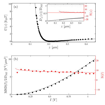
Fig. 5: TIRM with exponential intensity-distance relation. (a) The experimental (dots) and theoretical (solid line) potential. Inset: the diffusion coefficient on the position data (black dots) fits well Eq. (1) (black solid line), while the absolute value of the Brownian motion skewness $\mathrm{S}(z)$ is small (red dots). (b) Experimental $\mathrm{MSD}(I)$ (black dots) and skewness $\mathrm{S}(I)$ (red dots) for a scattering intensity time-series (polystyrene particle, $R=1.45\,\mu m$, $\rho_{p}=1.053\,g/cm^{3}$, $n_{p}=1.59$ suspended in water $n_{m}=1.33$ with $300\,\mu M$ NaCl background electrolyte, $\kappa^{-1}=17\,nm$, near a glass surface $n_{s}=1.52$, acquisition time $1800\,s$, sampling frequency $500\,Hz$) calculated using Eq. (4) and Eq. (5). Given the short penetration depth ($\beta=120\,nm$), the theoretical $\mathrm{MSD}(I)$ (black solid line) and $\mathrm{S}(I)$ (red solid line) for an exponential $I(z)$ fit the experimental ones and the conditions in Eqs. (6) are fulfilled.

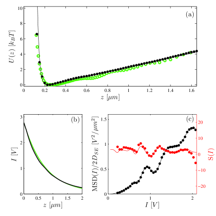
Fig. 6: TIRM with large penetration depth. (a) The experimental potential (black dots) obtained using the fitted intensity-distance relation and the theoretical one (black solid line). The green dots represent the faulty potential obtained using the exponential $I(z)$. (b) The fitted $I(z)$ (black line) and the exponential one (green line) corresponding to the penetration depth $\beta=720\,nm$. (c) Experimental intensity $\mathrm{MSD}(I)$ (black dots) and skewness $\mathrm{S}(I)$ (red dots) for a scattering intensity time-series (same particle and acquisition parameters as in Fig. 5) calculated using Eq. (4) and Eq. (5). Due to the large penetration depth, the $I(z)$ diverges from an exponential; the theoretical $\mathrm{MSD}(I)$ (black solid line) and $\mathrm{S}(I)$ (red solid line) correspond to the fitted $I(z)$.

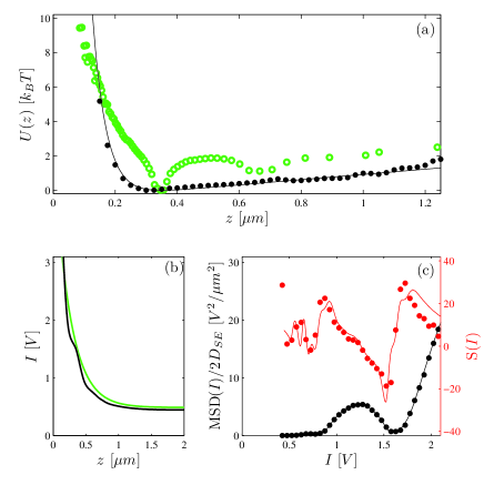
Fig. 7: TIRM in front of a reflective surface. (a) The experimental potential (black dots) obtained using the fitted intensity-distance relation and theoretical one (solid black line). The green dots represent the faulty potential obtained using the exponential $I(z)$ with $\beta=244\,nm$. (b) The fitted $I(z)$ (black line) and the exponential one (green line) corresponding to the evanescent field penetration depth $\beta=244\,nm$. (c) Experimental intensity $\mathrm{MSD}(I)$ (black dots) and skewness $\mathrm{S}(I)$ (red dots) for a scattering intensity time-series (same particle and acquisition parameters as in Fig. 5, except for background electrolyte $50\,\mu M$, $\kappa^{-1}=42\,nm$) calculated using Eq. (4) and Eq. (5). Due to the presence of a $20\,nm$-thick gold layer on the surface, the $I(z)$ deviates from an exponential; the theoretical $\mathrm{MSD}(I)$ (black solid line) and $\mathrm{S}(I)$ (red solid line) correspond to the fitted $I(z)$.

4.2 TIRM with large penetration depth

We now apply our technique under conditions where an exponential $I(z)$ is not valid, i.e. for large penetration depth as mentioned above. Fig. 6 shows the potential obtained for the same particle as in Fig. 5 but for a penetration depth ($\beta=720\,nm$). Note, that compared to 5 the potential extends over a much larger distance range since the particle’s motion can be tracked from hundreds of nanometers to microns. The green data points show the faulty interaction potential that is obtained when assuming an exponential $I(z)$. Since the only difference is in the illumination, the same potential as in Fig. 5 should be retrieved (solid line in Fig. 6(a)). However, applying an exponential $I(z)$ (green line in Fig. 6(b)) wiggles appear in the potential (green dots in Fig. 6(a)). Their origin is due to multiple reflections between the particle and the wall as discussed in detail in [21]. The correct $I(z)$ (black line in Fig. 6(b)) is obtained with the algorithm proposed in the previous section: after 9 iterations the conditions in Eqs. (6) appear reasonably satisfied, as shown in Fig. 6(c). With this $I(z)$, we reconstructed the potential represented by the black dots in Fig. 6(a), in good agreement with the one in Fig. 5. It should be noticed that, even though the deviations of the correct $I(z)$ from an exponential function are quite small, this is enough to significantly alter the measurement of the potential. This again demonstrates the importance of obtaining the correct $I(z)$ for the analysis of TIRM experiments.

4.3 TIRM in front of a reflective surface

To demonstrate that our method is capable of correcting even more severe optical distortions, we performed measurements in front of a reflecting surface ($20\,nm$ gold-layer, reflectivity $\approx 60\%$, $\beta=244\,nm$). The experimental conditions are similar to the previous experiments. Only the salt concentration was lowered to avoid sticking of the particle to the gold surface due to van der Waals forces, leading to a larger electrostatic particle-surface repulsion, and the optical trap was not used. Using an exponential $I(z)$ (green line in Fig. 7(b)), we obtain the potential represented by the green dots in Fig. 7(a), which clearly features unphysical artifacts, e.g. spurious potential minima. After 27 iterations of the data analysis algorithm, the black $I(z)$ in Fig. 7(b) is obtained, which reasonably satisfies the criteria in Eqs. (6) (Fig. 7(c)). The reconstructed potential (black dots in Fig. 7(a)) fits well to theoretical predictions (solid line); in particular the unphysical minima disappear.

5 Conclusions & Outlook

TIRM is a technique which allows one to measure the interaction potentials between a colloidal particle and a wall with femtonewton resolution. So far, its applicability has been limited by the need for an a priori knowledge of the intensity-distance relation. $I(z)\propto\exp(-z/\beta)$ can safely be assumed only for short penetration depths of the evanescent field and transparent surfaces. This, however, poses considerable constraints to the experimental conditions and the range of forces where TIRM can be applied. Here, we have proposed a technique to determine $I(z)$ that relies only on the hydrodynamic particle-surface interaction (Eq. 1) and, differently from existing data evaluation schemes, makes no assumption on the functional form of $I(z)$ or on the wall-particle potential. This technique will particularly be beneficial for the extension of TIRM to new domains. Here, we have demonstrated TIRM with a very large penetration depth, which allows one to bridge the gap between surface measurements and bulk measurements, and TIRM in front of a reflecting (gold-coated) surface, which allows plasmonic and biological applications.

This new technique only assumes the knowledge of the particle radius, which is usually known within an high accuracy and can also be measured in situ [24], and the monotonicity of $I(z)$. Were $I(z)$ not monotonous, as it might happen for a metallic particle in front of a reflective surface, the technique can be adapted to use the information from two non-monotonous signals, e.g. the scattering from two evanescent fields with different wavelength [31]. We notice that the technique encounters its natural limits when Eq. (1) does not correctly describe the particle-wall hydrodynamic interactions. This may happen in situations when the stick boundary conditions do not apply or when the hydrodynamic interactions are otherwise altered, e.g. in a viscoelastic fluid.

Since the conditions in Eqs. (6) are fulfilled only by the correct $I(z)$, they permit a self-consistency check on the data analysis. Even when an exponential $I(z)$ is justified, errors that arise from the estimation of some parameters (e.g. the zero-intensity $I_{0}$ and the background intensity $b_{s}$) can be easily avoided by checking the consistency of the analyzed data with the aforementioned criteria. In principle, the analysis of TIRM data can be completely automatized, possibly providing the missing link for a widespread application of TIRM to fields, such as biology, where automated analysis techniques are highly appreciated.

The proposed technique can also be useful to determine the intensity-distance relation in all those situations where it is possible to rely on the knowledge of the system hydrodynamics, while the scattering is not accurately known. Often explicit formulas are available for the hydrodynamic interaction of an over-damped Brownian particle in a simple geometry, while complex numerical calculations are needed to determine its scattering. As a limiting case, this technique might also prove useful for the PFM technique working in bulk, where the diffusivity is constant. Indeed, under certain experimental conditions – e.g. using back-scattered light instead of the more usual forward-scattered light [36] – the intensity-distance relation can be non-trivial and it can be necessary to determine it experimentally.