How parameters and regularization affect the PNJL model phase diagram and thermodynamic quantities

Abstract

We explore the phase diagram and the critical behavior of QCD thermodynamic quantities in the context of the so-called Polyakov–Nambu–Jona-Lasinio model. We show that this improved field theoretical model is a successful candidate for studying the equation of state and the critical behavior around the critical end point. We argue that a convenient choice of the model parameters is crucial to get the correct description of isentropic trajectories. The effects of the regularization procedure in several thermodynamic quantities is also analyzed. The results are compared with simple thermodynamic expectations and lattice data.

I Introduction

Quantum chromodynamics (QCD) exhibits at zero temperature and chemical potential two remarkable features which play an essential role in our understanding of strong interaction phenomena: the fundamental degrees of freedom are colorless bound states of hadrons (quark confinement), and chiral symmetry is dynamically broken. As it is well known these features characterize the nonperturbative nature of the QCD vacuum. It is expected that, at large energy densities, the so-called QCD phase transition occurs: the interaction becomes weaker and weaker due to asymptotic freedom HalaszJSSV ; Shuryak2006 with the formation of a new state of matter, the quark gluon plasma (QGP), and chiral symmetry gets restored.

The study of the QCD phase diagram in the $(T,\mu$)-plane and the search for signatures of the QGP have attracted an intensive investigation over the last decades. The outputs of this research are expected to play an important role in our understanding of the evolution of the early universe and of the physics of heavy-ion collisions at the Brookhaven National Laboratory, and at LHC (CERN), in the future.

Various results from QCD inspired models indicate (see e.g. Refs. Barducci:1994PRD ; Stephanov:1996PRL ) that at low temperatures the transition may be first order for large values of the chemical potential; on the contrary a crossover is found for small chemical potential and large temperature. This suggests that the first order transition line may end when the temperature increases, the phase diagram thus exhibiting a (second order) critical endpoint (CEP) Schwarz:PRC1999 ; Buballa:2003PLB ; Costa:2007PLB ; Asakawa that can be detected Stephanov:1998PRL ; Hatta:2003PRD by a new generation of experiments with relativistic nuclei, as the CBM experiment (FAIR) at GSI. Fodor and Katz Karsch claim the values $T^{CEP}=162$ MeV and $\mu^{CEP}=360$ MeV for such a critical point, although its precise location is still a matter of debate Gavai:2005PRD . In the chiral limit it is found, in accordance with universality arguments, a tricritical point (TCP) in the phase diagram, separating the second order transition line from the first order one. So, the exploration of the critical region of the phase diagram of strongly interacting matter gains increasing attention, both experimentally and theoretically.

As an approach complementary to first-principle lattice simulations, one can consider several effective models. One of them is the Nambu–Jona-Lasinio (NJL) model, that is undoubtedly a useful tool for understanding chiral symmetry breaking but does not possess a confinement mechanism. As a reliable model that can treat both the chiral and the deconfinement phase transitions, we can consider the Polyakov loop extended NJL (PNJL) model Megias:2006PRD ; Pisa1 ; Ratti:2005PRD ; Muller . In the PNJL model the deconfinement phase transition is described by the Polyakov loop. This improved field theoretical model is fundamental for interpreting the lattice QCD results and extrapolating into regions not yet accessible to lattice simulations.

A nontrivial question in NJL type models is the choice of the parameter set and of the regularization procedure. In fact, one should keep in mind that this type of models are used not only to describe physical observables in the vacuum but also to explore the physics at finite temperature and chemical potential. As it is well known, the order of the phase transition on the axis of the $(T,\mu)$-plane is sensitive to the values of the parameters, most notably to the value of the ultraviolet cutoff needed to regularize the integrals. In the pure NJL model a large cutoff leads to a second order transition, a small cutoff to a first order one Klevansky . An interesting feature to be noticed is that the requirement of global accordance with physical spectrum is obtained with values of the cutoff for which the transition is first order on the $T=0$ axis and a smooth crossover on the $\mu=0$ axis of the phase diagram. However, it has also been shown that different parameter sets, although providing a reasonable fit of hadronic vacuum observables and predicting a first order phase transition, will lead to different physical scenarios at finite $T$ and $\mu$ Buballa:2004PR ; Costa:2003PRC . For instance, the absolute stability of the vacuum state at $T=0$ is not always insured.

The consequences of the choice of the parameter set for the scenarios in the $(T,\mu)$-plane have not been discussed in the framework of the PNJL model, where the most popular parameter set does not allow for the absolute stability of the vacuum at $T=0$. In the present work, our main goal is to analyze this problem and we will assume that the most reliable parametrization of both NJL and PNJL models positively predicts the existence of the CEP in the phase diagram, together with the formation of stable quark droplets in the vacuum state at $T=0$.

Finally, the physical relevance of our numerical solutions is insured by requiring the agreement with general thermodynamic requirements. In particular, we will verify that the correct description of isentropic lines is closely related with the parameter choice in the pure NJL sector.

Concerning the regularization of some integrals, since, as it has been noticed by several authors, the three dimensional cutoff is only necessary at zero temperature, the dropping of this cutoff at finite $T$ is carefully analyzed in this work: this procedure allows for the presence of high momentum quark states, leading to interesting physical consequences, as it has been shown in Costa:2008PRD2 , where the advantages and drawbacks of this regularization have been discussed. We will enlarge the use of this procedure to the PNJL model and discuss its influence on the behavior of several relevant observables.

Let us notice that the choice of a regularization procedure is a part of the effective modeling of QCD thermodynamic. Indeed the presence of high momentum quarks (no cutoff on the temperature dependent part of the loop integrals) is required to ensure that the entropy scales as $T^{3}$ at high temperature. Hence we found that a comprehensive study of the differences between the two regularization procedures (with and without cutoff on the quark momentum states at finite temperature) is necessary to have a better understanding of the PNJL model and the role of high momentum quarks around the phase transition. This is one of the main purposes of this paper.

This paper is organized as follows: In Sec. II we present the model and formalism starting with the deduction of the self-consistent equations. We also extract the equations of state and the response functions, and show the pertinence and physical relevance of a convenient choice of the parametrization and regularization procedures of the model. Section III is devoted to the study of the phase transition at zero temperature, showing the important role of the choice of parameters for the formation of quark droplets in mechanical equilibrium with the vacuum at zero pressure. In Sec. IV we study thermodynamical quantities that, compared with lattice results, point out the physically relevant regularization procedure at $T\neq 0$. The enlargement to $\mu\neq 0$ allows for the study of the phase diagram in the $(T,\mu)$-plane (Sec. V). In Sec. VI we discuss the important role of the choice of the model parameters for the correct description of isentropic trajectories. In Sec. VII we proceed to study the size of the critical region around the CEP and its consequences for the susceptibilities and critical exponents. Finally, some concluding remarks are presented in Sec. VIII.

II Model and formalism

II.1 Model Lagrangian and gap equations

The generalized Lagrangian of the quark model for $N_{f}=2$ light quarks and $N_{c}=3$ color degrees of freedom, where the quarks are coupled to a (spatially constant) temporal background gauge field (represented in term of Polyakov loops), is given by Pisa1 ; Ratti:2005PRD ; Fukushima:2008PRD :

$${\mathcal{L}_{PNJL}\,} = \bar{q}\,(\,i\,{\gamma}^{\mu}\,D_{\mu}\,-\,\hat{m})\,q+\frac{1}{2}\,g\,[\,{(\,\bar{q}\,q\,)}^{2}\,\,+\,\,{(\,\bar{q}\,i\,\gamma_{5}\,\vec{\tau}q\,)}^{2}\,]$$ (1)

$$- \mathcal{U}\left(\Phi[A],\bar{\Phi}[A];T\right),$$

where the quark fields $q\,=\,(u,d)$ are defined in Dirac and color spaces, and $\hat{m}=\mbox{diag}(m_{u},m_{d})$ is the current quark mass matrix. The pure NJL sector contains three parameters: the coupling constant $g$, the cutoff $\Lambda$, and the current quark mass $m=m_{u}=m_{d}$, to be determined (see Sec. II C) by fitting the experimental values of several physical quantities.

$a_{0}$			$a_{1}$			$a_{2}$			$a_{3}$			$b_{3}$			$b_{4}$
6.75			-1.95			2.625			-7.44			0.75			7.5

Table 1: Parameter set used for the Polyakov loop potential (2) and (3).

The quarks are coupled to the gauge sector via the covariant derivative $D^{\mu}=\partial^{\mu}-iA^{\mu}$. The strong coupling constant $g_{Strong}$ has been absorbed in the definition of $A^{\mu}$: $A^{\mu}(x)=g_{Strong}{\cal A}^{\mu}_{a}(x)\frac{\lambda_{a}}{2}$, where ${\cal A}^{\mu}_{a}$ is the SU${}_{c}(3)$ gauge field and $\lambda_{a}$ are the Gell–Mann matrices. Besides in the Polyakov gauge and at finite temperature $A^{\mu}=\delta^{\mu}_{0}A^{0}=-i\delta^{\mu}_{4}A^{4}$.

The Polyakov loop $\Phi$ (the order parameter of $\mathbb{Z}_{3}$ symmetric/broken phase transition in pure gauge) is the trace of the Polyakov line defined by: $\Phi=\frac{1}{N_{c}}{\langle\langle\mathcal{P}\exp i\int_{0}^{\beta}d\tau\,A_{4}\left(\vec{x},\tau\right)\ \rangle\rangle}_{\beta}$, where ${\langle\langle\ldots\rangle\rangle}_{\beta}$ with $\beta=1/T$ is the thermal expectation value in the grand canonical ensemble.

The pure gauge sector is described by an effective potential $\mathcal{U}\left(\Phi[A],\bar{\Phi}[A];T\right)$ that takes the form

$$\frac{\mathcal{U}\left(\Phi,\bar{\Phi};T\right)}{T^{4}} = -\frac{b_{2}\left(T\right)}{2}\bar{\Phi}\Phi-\frac{b_{3}}{6}\left(\Phi^{3}+{\bar{\Phi}}^{3}\right)+\frac{b_{4}}{4}\left(\bar{\Phi}\Phi\right)^{2}\;,$$ (2)

where

$$b_{2}\left(T\right) = a_{0}+a_{1}\left(\frac{T_{0}}{T}\right)+a_{2}\left(\frac{T_{0}}{T}\right)^{2}+a_{3}\left(\frac{T_{0}}{T}\right)^{3}.$$ (3)

The coefficients $T_{0}$, $a_{i}$ and $b_{i}$ of the Polyakov loop effective potential are chosen (see Table 1 and Ratti:2005PRD ) to reproduce, at the mean-field level, the results obtained in pure gauge lattice calculations.

From the Lagrangian (1) in the mean-field approximation it is straightforward (see Ref. Klevansky-review ) to obtain the constituent quark mass $M$ that is given by

$$M=m-2g\,\left\langle\bar{q}q\right\rangle,$$ (4)

where the quark condensate $\left\langle\bar{q}q\right\rangle$ has to be determined in a self-consistent way. So, taking already into account Eq. (4), the PNJL grand potential density in the mean-field approach is given by Ratti:2005PRD ; Hansen:2007PRD :

$$\Omega(\Phi,\bar{\Phi},M;T,\mu) = {\cal U}\left(\Phi,\bar{\Phi},T\right)+2g\,N_{f}\left\langle\bar{q}q\right\rangle^{2}-2N_{c}\,N_{f}\int\frac{\mathrm{d}^{3}\,{p}}{\left(2\pi\right)^{3}}\,{E_{p}}$$ (5)

$$+ 2N_{f}\,T\int\frac{\mathrm{d}^{3}\,{p}}{\left(2\pi\right)^{3}}\,\left[\ln N^{+}_{\Phi}\,(E_{p})\,+\,\ln\,N^{-}_{\Phi}\,(E_{p})\right],$$

where $E_{p}$ is the quasiparticle energy for the quarks, $E_{p}=\sqrt{{\vec{p}\,}^{2}+M^{2}}$, and by defining $E_{p}^{\pm}\,=\,E_{p}\,\mp\mu$, the upper sign applying for fermions and the lower sign for antifermions, the functions $N^{+}_{\Phi}$ and $N^{-}_{\Phi}$ are:

$$N^{+}_{\Phi}(E_{p}) \equiv \left[1+3\left(\Phi+\bar{\Phi}e^{-\beta\,E^{+}_{p}}\right)e^{-\beta\,E^{+}_{p}}+e^{-3\beta\,E^{+}_{p}}\right]^{-1}~{},\$$ (6)

$$N^{-}_{\Phi}(E_{p}) \equiv \left[1+3\left(\bar{\Phi}+\Phi e^{-\beta\,E^{-}_{p}}\right)e^{-\beta\,E^{-}_{p}}+e^{-3\beta\,E^{-}_{p}}\right]^{-1}~{}.\$$ (7)

It was shown in Ref. Hansen:2007PRD that all calculations in the NJL model can be generalized to the PNJL one by introducing the modified Fermi–Dirac distribution functions for particles and antiparticles:

$$f^{+}_{\Phi}(E_{p})=M^{+}_{\Phi}\,N^{+}_{\Phi},\hskip 5.69046pt\,M^{+}_{\Phi}\,=\,\left(\Phi\,+\,2\,\bar{\Phi}\,e^{-\beta\,E^{+}_{p}}\right)\,e^{-\beta\,E^{+}_{p}}\,+\,e^{-3\beta\,E^{+}_{p}}~{},$$ (8)

$$f^{-}_{\Phi}(E_{p})=M^{-}_{\Phi}\,N^{-}_{\Phi},\hskip 5.69046pt\,M^{-}_{\Phi}\,=\,\left(\bar{\Phi}\,+\,2\,\Phi\,e^{-\beta\,E^{-}_{p}}\right)\,e^{-\beta\,E^{-}_{p}}\,+\,e^{-3\beta\,E^{-}_{p}}~{}.$$ (9)

To obtain the mean-field equations we must search for the minima of the thermodynamical potential density (5) with respect to $\left\langle\bar{q}q\right\rangle$, $\Phi$ and $\bar{\Phi}$. In fact, by minimizing $\Omega$ with respect to $\left\langle\bar{q}q\right\rangle$, we obtain the equations for the quark condensate:

$$\left\langle\bar{q}q\right\rangle\,=\,-6\,\int\frac{\mathrm{d}^{3}\,{p}}{\left(2\pi\right)^{3}}\frac{M}{E_{p}}[\theta\,(\Lambda^{2}\,-\,{\vec{p}}^{2})\,-\,f^{+}_{\Phi}(E_{p})-f^{-}_{\Phi}(E_{p})]\,.$$ (10)

Let us stress that in the latter we used a cutoff $\Lambda$ only for the $T=0$ part of the integral (denoted case I in the following); one could put a global cutoff $\int_{0}^{\Lambda}$ (denoted case II in the above).

Furthermore, minimization of $\Omega$ with respect to $\Phi$ and $\bar{\Phi}$ provides, respectively, the two additional mean-field equations Hansen:2007PRD (the integral that appears has to be understood as $\int_{0}^{\infty}$ for case I and $\int_{0}^{\Lambda}$ for case II):

$$0 = \frac{T^{4}}{2}\left[-b_{2}(T)\bar{\Phi}-b_{3}\Phi^{2}+b_{4}\Phi\bar{\Phi}^{2}\right]$$ (11)

$$- 12\,T\int\frac{\mathrm{d}^{3}\,{p}}{\left(2\pi\right)^{3}}\left[e^{-2\beta\,E^{+}_{p}}\,N^{+}_{\Phi}\,+\,e^{-\beta\,E^{-}_{p}}\,N^{-}_{\Phi}\right]\,,$$

$$0 = \frac{T^{4}}{2}\left[-b_{2}(T)\Phi-b_{3}\bar{\Phi}^{2}+b_{4}\bar{\Phi}\Phi^{2}\right]$$ (12)

$$- 12\,T\int\frac{\mathrm{d}^{3}\,{p}}{\left(2\pi\right)^{3}}\left[e^{-\beta\,E^{+}_{p}}\,N^{+}_{\Phi}\,+\,e^{-2\beta\,E^{-}_{p}}\,N^{-}_{\Phi}\right]\,.$$

The solutions of the three coupled equations (4), (11) and (12) allow us to obtain the behavior of $M$, and the Polyakov loop expectation values as a function of $T$ and $\mu$.

II.2 Equations of state and response functions

From the thermodynamical potential $\Omega(T,\mu)$ one can derive equations of state which allow us to compare some of our results with observables that have become accessible in lattice QCD at nonzero chemical potential. The relevant observables are the (scaled) quark number density, defined as

$$\frac{\rho_{q}(T,\mu)}{T^{3}}=-\frac{1}{T^{3}}\left(\frac{\partial\Omega}{\partial\mu}\right)_{T}\,,$$ (13)

and the (scaled) “pressure difference” given by

$$\frac{\Delta p(T,\mu)}{T^{4}}=\frac{p(T,\mu)-p(T,0)}{T^{4}}\,.$$ (14)

As usual, the pressure, $p$, is defined such as its value is zero in the vacuum state Buballa:2004PR and, since the system is uniform, one has

$$p(T,\mu)=-\frac{\Omega(T,\mu)}{V}\,,$$ (15)

where $V$ is the volume of the system.

Our work also includes the study of the isentropic trajectories due to their relevance for the study of the thermodynamics of matter created in relativistic heavy-ion collisions. The equation of state for the entropy density, $s$, is given by

$$s(T,\mu)\,=\left(\frac{\partial p}{\partial T}\right)_{\mu}\,,$$ (16)

and the energy density, $\epsilon$, comes from the following fundamental relation of thermodynamics

$$\epsilon(T,\mu)\,=\,T\,s(T,\mu)\,+\,\mu\,\rho_{q}(T,\mu)\,-\,p(T,\mu)\,.$$ (17)

The energy density, as well as the pressure, is defined such that its value is zero in the vacuum state Buballa:2004PR .

The baryon number susceptibility $\chi_{q}$ and the specific heat $C$ are the response of the baryon number density $\rho_{q}(T,\mu)$ and the entropy density $s(T,\mu)$ to an infinitesimal variation of the quark chemical potential $\mu$ and temperature, given respectively by:

$$\chi_{q}=\left(\frac{\partial\rho_{q}}{\partial\mu}\right)_{T},\hskip 28.45274pt{\rm and}\hskip 28.45274ptC=\frac{T}{V}\left(\frac{\partial s}{\partial T}\right)_{\mu}.$$ (18)

These second order derivatives of the pressure are relevant quantities to discuss phase transitions, mainly the second order ones.

II.3 Model parameters and regularization schemes

As already stated, the pure NJL sector involves three parameters: the coupling constant $g$, the current quark mass $m$ and the cutoff $\Lambda$. These parameters are determined in the vacuum by fitting the experimental values of several physical quantities. We notice that the parameters $g$ and $\Lambda$ are correlated with each other: if we increase $g$ in order to provide a more significative attraction between quarks, we must also increase the cutoff $\Lambda$ in order to insure a good agreement with experimental results. In addition, the value of the cutoff itself does have some impact as far as the medium effects in the limit $T=0$ are concerned.

We remember that different parameterizations may give rise to different physical scenarios at $T=0$ and $\mu\neq 0$ Buballa:2004PR , even if they give reasonable fits to hadronic vacuum observables and predict a first order phase transition.

	$\Lambda$	$g$	$m$	($|\langle{\bar{\psi}}_{u}\psi_{u}\rangle|^{1/3}$	$f_{\pi}$	$m_{\pi}$	$M$
	[GeV]	[GeV-2]	[MeV]	[MeV]	[MeV]	[MeV]	[MeV]
Set A	( 0.590	7.0	6.0	241.5	92.6	140.2	400
Set B	( 0.651	5.04	5.5	251	92.3	139.3	335

Table 2: Set of parameters ($\Lambda,\,g,\,m$) used in the NJL sector of the PNJL model and the physical quantities chosen to fix the parameters. The constituent quark mass obtained is also included.

Here, we will use two different sets of parameters whose values are presented in Table 2. These two sets are the most widely used in NJL type models: set A is taken from Buballa:2003PLB and set B from kunihiro , the last one being commonly used in the context of the PNJL model Ratti:2005PRD ; Hansen:2007PRD . The main feature is a lower (larger) value of the cutoff for set A (B), for which we verify that $\Lambda/M<1.8$ ($>1.8$). We notice that the transition between the regime of stable to the regime of metastable quark matter occurs at the value $\Lambda/M\approx 1.8$ fiolhais . So, we will prove that only the set of parameters A insures the stability conditions and, consequently, the compatibility with thermodynamic expectations. We notice that set A also agrees with an empirical relation derived in Buballa:1996NPA which states that stable quark matter is only possible in NJL model if $M>4f_{\pi}$.

On the other hand, the regularization procedure, as soon as the temperature effects are considered, has relevant consequences on the behavior of physical observables, namely on the chiral condensates and the meson masses Costa:2008PRD3 . In PNJL model, the two types of regularization may be found Ratti:2005PRD ; Hansen:2007PRD ; Sasaki ; Kashiwa:2008PLB ; Alb2009 as well as different sets of parameters Ratti:2005PRD ; Hansen:2007PRD ; Costa:2008PRD3 ; Sasaki ; Kashiwa:2008PLB . So, in order to compare the differences between the use of different sets of parameters and of regularization schemes, in the physical scenarios of the PNJL model, we will consider sets A and B of parameters and two different regularization procedures at $T\neq 0$:

Case I. — The cutoff is used only in the integrals that are divergent ($\Lambda\rightarrow\infty$ in the convergent ones; see Eqs.(10, 11, 12) for example) at finite temperature, a procedure that allows us to take into account the effects of high momentum quarks Ratti:2005PRD ; Klevansky ; Sasaki ; Mish2000 .

Case II. — The regularization consists in the use of the cutoff $\Lambda$ in all integrals Hansen:2007PRD ; Kashiwa:2008PLB .

Advantages and drawbacks of these regularization procedures have been discussed in Costa:2008PRD2 . Here, our main goal is to show nontrivial consequences of the regularization scheme used in case I. We remind that the main drawback of this regularization is that at high temperature there is a too fast decrease of the quark masses that become lower than their current values. This leads to a non physical behavior of the quark condensates that, after vanishing at the point where constituent and current quark masses coincide, changes sign and acquires a nonzero value again. Therefore, if we want to keep calculating observables in this region, it seems sensible to impose the condition that the quark masses take their current values and the quark condensates remain zero. This is the approach used here.

III Phase transition at zero temperature

Our study refers mainly to the finite temperature case. However, the particular case of zero temperature is very important due to the possibility of having, simultaneously, a vanishing density and a finite chemical potential. This feature depends on the choice of the parameters and is necessary in order to insure the satisfaction of general thermodynamic requirements.

Here we analyze the stability of the quark matter at $T=0$. For this special case the PNJL model reduces to the NJL one. We will now present a discussion about the stability of the system along the same lines of Buballa:2004PR ; Costa:2003PRC ; Costa:2008PRD1 , which will allow us to choose the set of parameters corresponding to the most convenient physical situation.

In the limit $T\rightarrow 0$ the normal Fermi-Dirac distribution function reduces to the step function

$$\theta(\mu\,-\,E_{p})\,=\,\theta(p_{F}-p)\,\theta(\mu\,-\,M),$$ (19)

where the Fermi momentum is given by

$$p_{F}\,=\,\sqrt{\mu^{2}\,-\,M^{2}}\,\theta(\mu\,-\,M)\,=\,(\pi^{2}\,\rho_{q})^{1/3}\,\theta(\mu\,-\,M).$$ (20)

The important point of our argumentation about the choice of the model parameters comes from the comparison between the point $(0,\mu_{c})$ of the phase diagram, where $\mu_{c}$ is the position of the first order line at zero temperature, and the point $(0,M_{vac})$, where $M_{vac}=M$ is the mass of the $u,d$-quark in the vacuum. Two special cases are observed Buballa:2004PR :

• For set A, the first order phase transition occurs at $\mu_{c}$ such that $\mu_{c}<M_{vac}$, and consequently (see Eq. 20) the phase transition connects the vacuum state ($\rho_{q}=0$) directly with the phase of partially restored chiral symmetry ($\rho_{q}=\rho_{c}$).

• For set B, $\mu_{c}>M_{vac}$, so the phase transition connects a $\rho_{q}\neq 0$ phase of massive quarks with the phase of partially restored chiral symmetry ($\rho_{q}=\rho_{c}$).

So, although we can choose several sets of parameters which fit physical observables in the vacuum, we notice, however, that the value of the cutoff itself does have some impact on the characteristic of the first order phase transition. Comparing the two sets of parameters we verify that for larger values of the cutoff, as in set B, a more strong attraction is necessary both to reproduce the physical values in the vacuum and to insure a first order phase transition. As we will argue in the sequel, the more reliable case is provided by set A.

In case (i) the energy per particle reaches, at $\rho_{q}=\rho_{c}$, an absolute minimum $\epsilon<\epsilon(0)\,=\,M_{vac}$. This is compatible with the existence of stable quark matter, indicating the possibility for finite droplets to be in mechanical equilibrium with the vacuum at zero pressure Buballa:2004PR ; Costa:2003PRC ; Mish2000 ; Rajagopal:1999NPA . This is due to the fact that the pressure has three zeros, respectively at $\rho=0,\,0.52\rho_{0},\,4.3\rho_{0}$ ($\rho_{0}=0.17$ fm^-3), that correspond to extrema of the energy per particle. The third zero of the pressure, located at $\rho_{c}=4.3\rho_{0}$, corresponds to an absolute minimum of the energy. The critical point of the phase transition in these conditions satisfies to $\mu_{c}<M_{vac}$ Buballa:2004PR ; Scavenius . This can be seen by comparing $\mu_{c}=383$ MeV with the quark masses $M_{vac}\,=\,M\,=\,400$ MeV. Above $\rho_{q}=\rho_{c}$, we have again a uniform gas phase. For densities $0<\rho_{q}<\rho_{c}$ the equilibrium configuration is a mixed phase, where the equality of all intensive variables ($T$, $P$ and $\mu$) defines the condition for the phase equilibrium. So, the Gibbs criterion is satisfied and the phase transition is a first order one Buballa:2004PR ; Costa:2008PRD1 .

On the contrary, the minimum at $\rho_{q}=\rho_{c}$ in case (ii) corresponds to metastable quark matter, since $\epsilon>\epsilon(0)\,=\,M_{vac}$. The pressure still has three zeros, respectively at $\rho_{q}=0,\,1.51\rho_{0},\,2.64\rho_{0}$, that correspond to extrema of the energy per particle. The main difference now is that the absolute minimum of the energy per particle is at $\rho_{q}=0$. This means that, in spite of being in the presence of a first order phase transition, there are no droplets in mechanical equilibrium with the vacuum at zero pressure. In addition, from the physical point of view, this scenario is unrealistic because it predicts the existence of a low-density phase of homogeneously distributed constituent quarks Buballa:2004PR . Other implications of this scenario on the reliability of isentropic trajectories will be discussed later.

IV Thermodynamic quantities

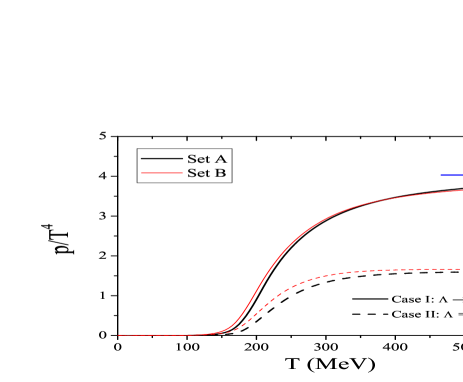
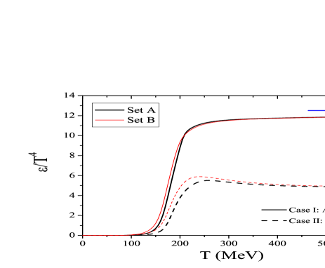
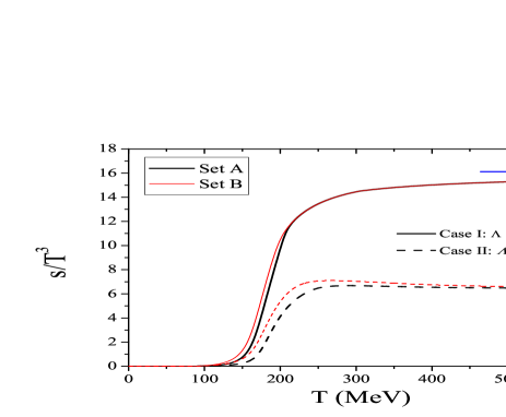
Figure 1: Scaled pressure $(p)$, energy per particle $(\epsilon)$, and entropy $(s)$ as a function of the temperature at zero chemical potential for both sets of parameters A and B, and both regularization procedures.

A significative information on the phase structure of QCD at high temperature is obtained from lattice calculations in the limit of vanishing quark chemical potential. The transition to the phase characteristic of this regime is related with chiral and deconfinement transitions which are the main features of our model calculation.

Following the argumentation presented in Ratti:2005PRD , we use the reduced temperature $T_{c}$ by rescaling the parameter $T_{0}$ from 270 to 190 MeV (we do this rescaling only for the remainder of this section). In this case we loose the perfect coincidence of the chiral and deconfinement transitions: they are shifted relative to each other by less than 35 (30) MeV for set A (B). As in Ref. Ratti:2005PRD , we define $T_{c}$ as the average of the two transition temperatures: we have $T_{c}=190\,(184)$ MeV for set A (B) within the range expected from lattice calculations Karsch2 .

For comparison purposes with lattice findings, we start by considering our numerical results at vanishing quark chemical potential by checking the usefulness of the present regularization procedure, case I. To this purpose, we plot the scaled pressure, the energy and the entropy as functions of the temperature in Fig. 1.

The transition to the high temperature phase is a rapid crossover rather than a phase transition and, consequently, the pressure, the entropy and the energy densities are continuous functions of the temperature. For case I we observe a similar behavior in the three curves: a sharp increase in the vicinity of the transition temperature and then a tendency to saturate at the corresponding ideal gas limit. Asymptotically, the QCD pressure for $N_{f}$ massless quarks and $(N_{c}^{2}-1)$ massless gluons is given, for $\mu=0$, by

$$\frac{p_{SB}}{T^{4}}\,=\,(N_{c}^{2}-1)\,\frac{\pi^{2}}{45}\,+\,N_{c}\,N_{f}\,\frac{7\,\pi^{2}}{180},$$ (21)

where the first term denotes the gluonic contribution and the second term the fermionic one.

Our results follow the expected tendency and go to the free gas values, a feature that was also found with this type of regularization in the context of the PNJL model Megias:2006PRD ; Ratti:2005PRD . For what concerns the NJL model Klevansky let us notice that if indeed a tendency to saturate is found, the asymptotic value is at about half the ideal gas limit. Hence the inclusion of the Polyakov loop effective potential ${\cal U}(\Phi,\bar{\Phi})$ (it can be seen as an effective pressure term mimicking the gluonic degrees of freedom of QCD) is required to get the correct limit.

The inclusion of the Polyakov loop together with the regularization procedure implemented in case I, is essential to obtain the required increase of extensive thermodynamic quantities, insuring the convergence to the Stefan-Boltzmann (SB) limit of QCD lattice1 . Some comments are in order concerning the role of the regularization procedure for $T>T_{c}$. In this temperature range, due to the presence of high momentum quarks, the physical situation is dominated by the significative decrease of the constituent quark masses by the $q\bar{q}$ interactions. This allows for an ideal gas behavior of almost massless quarks with the correct number of degrees of freedom.

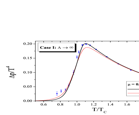
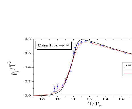
Figure 2: Comparison of the scaled pressure difference (left panel) and the scaled quark number density (right panel), as a function of temperature at finite chemical potential for sets A and B, with the lattice data taken from Ref. lattice2 .

The advantage of our phenomenological model is the possibility to provide equations of state at nonzero chemical potential too. So, we can also test its ability to reproduce recent progress in lattice QCD with small non vanishing chemical potential.

In order to do this, we plot in Fig. 2 the scaled pressure and the quark number density for $\mu=0.6\,T_{c}$ (it was done in Ratti:2005PRD for set B). The parameters are the same as in Fig. 1 and only case I for the cutoff procedure is considered. The agreement with the lattice data is fairly good, showing that the general pattern of these quantities and the behavior at large $T$ is reproduced. The more significative deviations are observed in the scaled baryon number density at intermediate temperatures as is evident from Fig. 2 (right side). However, there are some advantage with respect to the employed parametrization A, where an improvement of the results is observed as shown in the left panel of Fig. 2.

In conclusion, by introducing finite chemical potential we are able to compare the obtained results with lattice data and check the validity of both sets of parameters. From Fig. 2 we conclude that, for case I, both sets of parameters are in good agreement with lattice results, in particular, to $\Delta p/T^{4}$ and $\rho_{q}/T^{3}$ at $\mu=0.6\,T_{c}$.

V Phase structure

The phase diagram for both sets of parameters (see Fig. 3) is determined by the behavior of the orderlike parameters $\left\langle\bar{q}\,q\right\rangle$, $\Phi$ and $\bar{\Phi}$ together with the grand canonical potential as a function of temperature and chemical potential. To draw the phase diagram we will use $T_{0}=270$ MeV as given by pure gauge lattice calculations, a choice that ensures the very important physical outcomes of lattice calculations that chiral and deconfinement transitions coincide in the PNJL model..

We start our analysis in the limit $T=0$, where the first order phase transition occurs at the same chemical potential for both cases I and II: $\mu=383\,(344)$ MeV for set A (B). This is due to the fact that at $T=0$ all the integrals are regularized with the cutoff $\Lambda$. As a matter of fact, in this limit the Fermi functions in the gap equations become a step function of the form $\theta(\Lambda-p_{F})$ where $p_{F}$ is the hadronic matter Fermi momentum. So, the integration occurs between $p_{F}$ and $\Lambda$ for both cases.

From Fig. 3 we also see that, at $\mu=0$, the crossover takes place for set A at $T=235\,(272)$ MeV for case I (II), while for set B the crossover takes place at $T=229\,(256)$ MeV for case I (II).

Parameter	Regularization	$T^{CEP}$	$\mu^{CEP}$	$T^{TCP}$ [MeV]	$\mu^{TCP}$ [MeV]
set	procedure	[MeV]	[MeV]	(chiral limit)	(chiral limit)
Set A	Case I: $\Lambda\rightarrow\infty$	172.48	286.35	206.50	192.87
	Case II: $\Lambda\,=\,const$	169.11	321.32	207.66	270.80
Set B	Case I: $\Lambda\rightarrow\infty$	87.99	328.84	162.39	253.06
	Case II: $\Lambda\,=\,const$	87.71	329.51	163.06	268.05

Table 3: Location of the CEP and the TCP at the $(T,\mu)$-plane for both sets of parameters and regularization procedures.

At nonzero chemical potential, as the temperature increases, it is well know that the first order transition persists up to the CEP. At the CEP the chiral transition becomes of second order. For temperatures above the CEP a smooth crossover takes place.

These general characteristics are qualitatively similar for both cases, in the two sets of parameters, as it was expected. The relevant point is the distance between the CEP’s, in cases I and II, is bigger for set A than for set B. This is due to fact that the CEP’s for set A are at a higher temperature than for set B. As the temperature increases, the high momentum quarks, that are taken into account in case I ($\Lambda\rightarrow\infty$), are more and more relevant leading to a visible splitting of the lines of first order phase transition and, consequently, to other location of the CEP in the phase diagram. For set B this splitting is smaller, once lower critical temperatures are observed. In the chiral limit ($m=0$ and $m_{\pi}=0$), the transition is of second order at $\mu=0$ and, as $\mu$ increases, the line of second order phase transition will end in a first order line at the TCP. The location of the tricritical points are also included in Table 3. Nevertheless, in this case, the TCP is located at higher temperature than the CEP (see Fig. 3, right panel), and we already see a bigger shift between them.

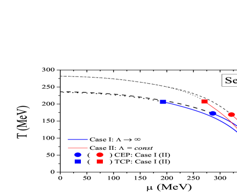
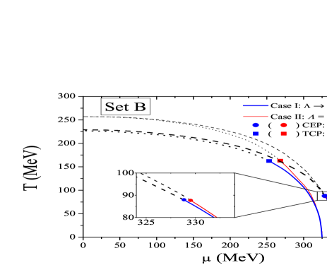
Figure 3: Phase diagrams for cases I and II in the chiral limit (boxes) or not (circles) using the parameters set A (left panel) and B (right panel). The solid part of the curves denotes a first order transition, the dashed part to the second order transition and the dotted line the crossover transition.

VI Nernst principle and isentropic trajectories

The isentropic lines play a very important role in the understanding of thermodynamic properties of matter created in relativistic heavy ion collisions. Most of the studies on this topic have been done on lattice calculations for two flavor QCD at finite $\mu$ Ejiri:2006PRD but there are also studies using different type of models Scavenius ; Nonaka:2005PRC ; Kahara:2008 . Some model calculations predict that in a region around the CEP the properties of matter are only slowly modified as the collision energy is changed, as a consequence of the attractor character of the CEP Stephanov:1998PRL .

Our numerical results for the isentropic lines in the $(T,\mu)$-plane are shown in Fig. 4, where we have used set A of parameters and both regularization procedures.

We start the discussion by analyzing the behavior of the isentropic lines in the limit $T\rightarrow 0$. We point out that, as already referred by other authors Scavenius , in this limit:

• $s\rightarrow 0$, according to the third law of thermodynamics; and

• for $s/\rho_{q}\,=\,const$, we have to insure that also $\rho_{q}\rightarrow 0$.

However, the satisfaction of the condition (ii) is only provided when $\mu\leq M_{vac}$. In spite of the general use of set B in the literature of the PNJL model, only set A satisfies this ansatz. We remember (Sec. 2.3) that with set A we are, at $T=0$, in the presence of droplets (states in mechanical equilibrium with the vacuum state at $P=0$).

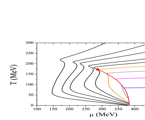
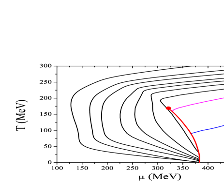
Figure 4: Isentropic trajectories in the $(T,\mu)$-plane for case I (left panel) and case II (right panel) using the parameter set A. The following values of the entropy per baryon number have been considered: $s/\rho_{q}=1,\,2,\,3,\,4,\,5,\,6,\,8,\,10,\,15$ (anticlockwise direction).

Consequently, even without reheating in the mixed phase as verified in the “zigzag” shape of Ejiri:2006PRD ; Nonaka:2005PRC ; Kahara:2008 ; Subramanian , all isentropic trajectories directly terminate at the first order transition line at $T=0$. So, for set A it is verified that $s\rightarrow 0$ and $\rho_{q}\rightarrow 0$ in the limit $T\rightarrow 0$, as it should be.

In conclusion, our convenient choice of the model parameters allows a first order phase transition that is stronger than in other treatments of the NJL (PNJL) model. This choice is crucial to obtain important results: the criterium of stability of the quark droplets Buballa:2004PR ; Costa:2003PRC is fulfilled, and, in addition, simple thermodynamic expectations in the limit $T\rightarrow 0$ are verified.

At $T\neq 0$, in the first order line, the behavior we find is somewhat different from those claimed by other authors Nonaka:2005PRC ; Stephanov:1999PRD where a phenomena of focusing of trajectories towards the CEP is observed. For case I (see Fig. 4, left panel) we see that the isentropic lines with $s/\rho_{q}=1,...,4$ come from the region of symmetry partially restored and attain directly the phase transition, going along with the phase transition as $T$ decreases until it reaches $T=0$. The same behavior is found for case II when $s/\rho_{q}=1,2$ (see Fig. 4, right panel). For case II, we also observe, in a small range of $s/\rho_{q}$ around $3$, a tendency to convergence of these isentropic lines towards the CEP. These lines come from the region of symmetry partially restored in the direction of the crossover line. For smaller values of $s/\rho_{q}$, the isentropic lines turn about the CEP and then attain the first order transition line. For larger values of $s/\rho_{q}$ the isentropic trajectories approach the CEP by the region where the chiral symmetry is still broken, and also attain the first order transition line after bending toward the critical point. As already pointed out in Scavenius , this is a natural result in these type of quark models with no change in the number of degrees of freedom of the system in the two phases. As the temperature decreases a first order phase transition occurs, the latent heat increases and the formation of the mixed phase is thermodynamically favored.

In the crossover region, for both cases, the behavior of the isentropic lines is qualitatively similar to the one obtained in lattice calculations Ejiri:2006PRD or in some models Nonaka:2005PRC ; Fukushima ; Nakano . On the other hand, the isentropic trajectories in the phase diagram indicate that the slope of the trajectories goes to large values for large $T$. We can also conclude that, in the PNJL model, the entropy and the baryon number density are very sensitive to the regularization procedure used Klevansky ; Costa:2008PRD2 , and this effect is also relevant for the present situation.

VII Susceptibilities and critical exponents

The grand canonical potential (or the pressure) contains the relevant information on thermodynamic bulk properties of a medium. Susceptibilities, being second order derivatives of the pressure in both chemical potential and temperature directions, are related to fluctuations that are supposed to represent signatures of phase transitions of strongly interacting matter. In particular, the quark number susceptibilities play a role in the calculation of event-by-event fluctuations of conserved quantities such as net baryon number. Across the quark hadron phase transition they are expected to become large, what can be interpreted as an indication for a critical behavior. We also remember the important role of the second derivative of the pressure for second order points like the CEP.

In previous works Costa:2008PRD3 ; Costa:2008PRD1 , we have studied the CEP within the restrictions imposed by the regularization in case II. It is important to investigate if the type of regularization plays a significant role in the critical properties of physical observables, such as the baryon number susceptibility and the specific heat, and respective critical exponents, in the vicinity of the CEP. The relevance of these physical observables is due to the size of the critical region around the CEP which can be found by calculating the baryon number susceptibility, the specific heat and their critical behaviors. The size of this critical region is important for future searches of the CEP in heavy ion-collisions Nonaka:2005PRC .

In our calculations, we will use only the set A of parameters due to the advantages of this set as explained in the previous sections. In Fig. 5 we plot the phase diagram in a region around the CEP for both cases.

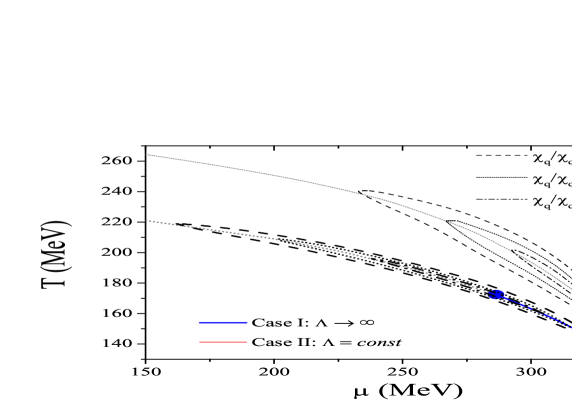
Figure 5: Phase diagram in the PNJL (case I and case II) for the parameter set A. The size of the critical region around the CEP is plotted for $\chi_{q}/\chi_{q}^{free}=2,3,5$.

The way to estimate the critical region around the CEP is to calculate the dimensionless ratio $\chi_{q}/\chi_{q}^{free}$, where $\chi_{q}^{free}$ is obtained taking the chiral limit $m=0$. Figure 5 shows a contour plot for three fixed ratios ($\chi_{q}/\chi_{q}^{free}=2.0,\,3.0,\,5.0$) in the phase diagram around the CEP. We notice an elongation, in the direction parallel to the first order transition line, of the region where $\chi_{q}$ is enhanced, indicating that the critical region is heavily stretched in that direction.

The elongation of the critical region in the $(T,\mu)$-plane, along the line of the phase transition (or the crossover), is larger in case I (see for example $\chi_{q}/\chi_{q}^{free}=2.0$ in Fig. 5). It means that the divergence of the correlation length at the CEP affects the phase diagram quite far from the CEP, particularly in case I, and a careful analysis including effects beyond the mean-field needs to be done Rossner:2007ik .

We remember that one of the main effects of the Polyakov loop is to shorten the temperature range where the crossover occurs Hansen:2007PRD . On the other hand, this behavior is boosted by using $\Lambda\rightarrow\infty$: at $\mu=0$ the crossover occurs between about 180 MeV and 270 MeV, for case I, and between about 210 MeV and 325 MeV, for case II. The combination of both effects results in higher baryonic susceptibilities even far from the CEP. This effect of the Polyakov loop is driven by the fact that the one- and two-quark Boltzmann factors are controlled by a factor proportional to $\Phi$: at small temperature $\Phi\simeq 0$ results in a suppression of these contributions (see Eq. 5) leading to a partial restoration of the color symmetry. Indeed, the fact that only the $3-$quarks Boltzmann factors $e^{3\beta E_{p}}$ contribute to the thermodynamical potential at low temperature, may be interpreted as the production of a thermal bath containing only colorless 3-quarks contributions. When the temperature increases, $\Phi$ goes quickly to 1 (this is faster in case I due to the higher momentum quarks present in the system) resulting in a (partial) restoration of the chiral symmetry occurring in a shorter temperature range. The crossover taking place in a smaller $T$ range can be interpreted as a crossover transition closest to a second order one, a feature that is more clear in case I than in case II. This “faster” crossover may explain the elongation of the critical region in case I, compared to case II, giving raise to a greater correlation length even far from the CEP.

Now, we will investigate the behavior of $\chi_{q}$ and $C$ in the vicinity of the CEP and their critical exponents, for both cases. The calculated critical exponents at the CEP and the TCP, together with the universality/mean-field predictions, are presented in Table 4 and will be discussed in the sequel.

Quantity	critical exponents/path	Case I	Case II	Universality
	$\epsilon\,/\,\,{\rm from\,left\,({{\color[rgb]{1,0,0}\Rightarrow}})}$	$0.66\pm 0.01$	$0.66\pm 0.01$	$2/3$
$\chi_{q}$	$\epsilon^{\prime}\,/\,$ from right $({{\color[rgb]{1,0,0}\Leftarrow}})$	$0.69\pm 0.01$	$0.69\pm 0.02$	$2/3$
	$\gamma_{q}$ $\,/$ from left $({{\color[rgb]{0,0,1}\rightarrow}})$	$0.53\pm 0.02$	$0.51\pm 0.01$	$1/2$
	$\alpha\,/$ from below ${({{\color[rgb]{1,0,0}\Uparrow})}}$	$\begin{array}[]{c}0.64\pm 0.01\\ \alpha_{1}=0.58\pm 0.01\end{array}$	$\begin{array}[]{c}0.62\pm 0.02\\ \alpha_{1}=0.52\pm 0.01\end{array}$	$\begin{array}[]{c}2/3\\ $---$\end{array}$
$C$	$\alpha^{\prime}/$ from above $({{\color[rgb]{1,0,0}\Downarrow}})$	$0.68\pm 0.01$	$0.68\pm 0.01$	$2/3$
	$\alpha$ $\,/$ from below $({{\color[rgb]{0,0,1}\uparrow}})$	$0.50\pm 0.01$	$0.47\pm 0.02$	$1/2$

Table 4: The arrow ${{\color[rgb]{1,0,0}\Rightarrow}}({{\color[rgb]{0,0,1}\uparrow}})$ indicates the path in the $\mu\,(T)-$ direction to the CEP/TCP for ${\mu<\mu^{CEP}}$ $({T<T^{TCP}}$).

In the left panel of Fig. 6 the baryon number susceptibility is plotted as a function of $\mu$ for three different temperatures around the CEP in the context of case I. The behavior is very similar in both cases. For $T<T^{CEP}$, the phase transition is first order and $\chi_{q}$ has a discontinuity; for $T=T^{CEP}$, the slope of the baryon number density tends to infinity at $\mu=\mu^{CEP}$ and $\chi_{q}$ diverges; for $T>T^{CEP}$, the discontinuity of $\chi_{q}$ disappears at the transition line. A similar behavior of $\chi_{q}$ is found for case II, as we can see from the right panel of Fig. 6.

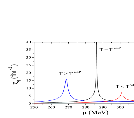
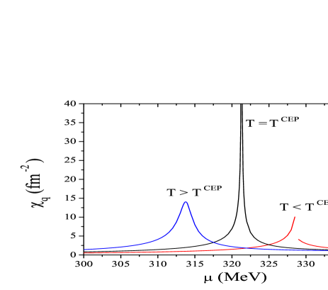
Figure 6: Left panel: Baryon number susceptibility for case I as function of $\mu$ for different temperatures around the CEP: $T^{CEP}=172.48$ MeV and $T=T^{CEP}\pm 10$ MeV. Right panel: Baryon number susceptibility for case II as function of $\mu$ for different temperatures around the CEP: $T^{CEP}=169.11$ MeV and $T=T^{CEP}\pm 10$ MeV.

The behavior of the specific heat for both cases, as a function of temperature for three different chemical potentials around the CEP, is presented in Fig. 7. The behavior found for $C$ around the CEP is very similar to the behavior of $\chi_{q}$ for both Cases as we can see from Fig. 7.

It is interesting to notice that the high momentum quarks introduced in case I ($\Lambda\rightarrow\infty$), and that are not taken into account in case II, have no significant effect on both $\epsilon$ and $\alpha$. However, we observe that the peak at the critical points $T^{CEP}$ or $\mu^{CEP}$ is sharper in the PNJL model in case I (as it can be expected from the analysis of the stretching of the critical region done above).

To better understand the extreme behavior of $\chi_{q}$ and $C$ near the CEP, we will determine the critical exponents (in our case $\epsilon$ and $\alpha$ are the critical exponents of $\chi_{q}$ and $C$, respectively). These critical exponents will be determined by following two directions, temperature-like and magnetic-field-like, in the $(T,\mu)$-plane near the CEP, because, as pointed out in Griffiths:1970PR , the form of the divergence depends on the route that is chosen to approach the CEP.

Starting with the baryon number susceptibility, for both cases, if the path chosen is asymptotically parallel to the first order transition line at the CEP, the divergence of $\chi_{q}$ scales with an exponent $\gamma_{q}$. In the mean-field approximation it is expected to find $\gamma_{q}=1$ for this path. For directions not parallel to the tangent line, the divergence scales as $\epsilon=2/3$. These values are responsible for the elongation of the critical region, $\chi_{q}$ being enhanced in the direction parallel to the first order transition line (see Fig. 5).

To study the critical exponents for the baryon number susceptibility (Eq. 18) we will start with a path parallel to the $\mu$-axis in the ($T,\mu$)-plane, from lower $\mu$ towards the CEP ($T^{CEP},\mu^{CEP}$). Using a linear logarithmic fit $\ln\chi_{q}=-\epsilon\ln|\mu-\mu^{CEP}|+c_{1}$, where the term $c_{1}$ is independent of $\mu$, we obtain $\epsilon=0.66\pm 0.01$, which is consistent with the mean-field theory prediction, $\epsilon=2/3$. This value is also similar to the value found in case II as we can see from Table 4 (see also Ref. Costa:2008PRD3 ).

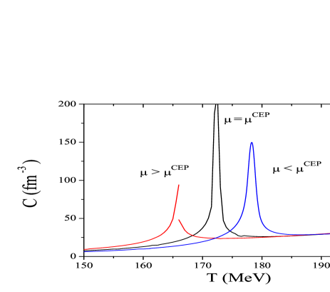
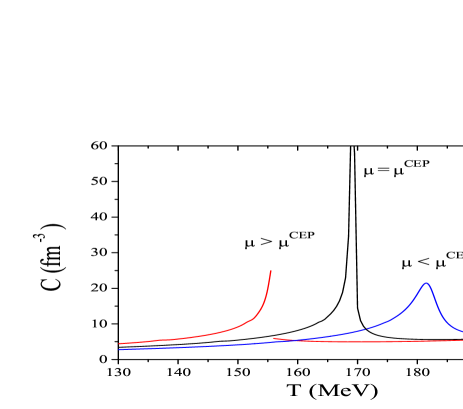
Figure 7: Left panel: Specific heat for case I as a function of $T$ for different values of $\mu$ around the CEP: $\mu^{CEP}=286.35$ MeV and $\mu=\mu^{CEP}\pm 10$ MeV. Right panel: Specific heat for case II as a function of $T$ for different values of $\mu$ around the CEP: $\mu^{CEP}=321.32$ MeV and $\mu=\mu^{CEP}\pm 10$ MeV.

We also study the baryon number susceptibility from higher $\mu$ towards the critical $\mu^{CEP}$ for both cases. The logarithmic fit used now is $\ln\chi_{q}=-\epsilon^{\prime}\ln|\mu-\mu^{CEP}|+c^{\prime}_{1}$. Our result for case I shows that $\epsilon^{\prime}=0.69\pm 0.01\approx\epsilon$. This means that the size of the region we observe is approximately the same independently of the direction we choose for the path parallel to the $\mu$-axis. Once again, this value is similar to the critical exponent for case II and is consistent with the mean-field theoretical prediction $\epsilon=2/3$ (see the results presented in Table 4).

On the other hand, in the chiral limit (where the CEP becomes a TCP), it is found that the critical exponent for $\chi_{q}$, denoted by $\gamma_{q}$, has the value $\gamma_{q}=0.53$ $\pm 0.02$ ($\gamma_{q}=0.51$ $\pm 0.01$), for case I (II). Again, these results are in agreement with the mean-field value ($\gamma_{q}=1/2$).

Let us pay attention to the specific heat around the CEP. We can calculate the critical exponent using a path parallel to the $T$-axis in the ($T,\mu$)-plane from lower $T$ towards the CEP. We observe that, as already found in Ref. Costa:2008PRD3 for case II, the slope of data points change for $|T-T^{CEP}|$ around $0.3$ MeV. So, for case I (II) we obtain the critical exponents $\alpha=0.64\pm 0.01\,(0.62\pm 0.02)$ and $\alpha_{1}=0.58\pm 0.01\,(0.52\pm 0.01)$. As pointed out in Hatta:2003PRD , this change of the exponent can be interpreted as a crossover of different universality classes, with the CEP being affected by the TCP due to the small physical quark masses.

The value of $\alpha$ in both cases is consistent with the one suggested by universality arguments in Hatta:2003PRD : it is expected that $\chi_{q}$ and $C$ should be essentially the same near the TCP and the CEP which implies $\alpha=\epsilon=2/3$. In addition, if we compare $\alpha_{1}$ for both cases, we conclude that $\alpha_{1}$ in case I is closer to $\alpha$ than in case II. It seems that the high momentum quarks allowed in case I affect the crossover of different universality classes making $\alpha_{1}$ getting closer to $\alpha$ which is already consistent with $\alpha=\epsilon=2/3$

When the critical point is approached from above the following exponents are obtained: $\alpha^{\prime}=0.68\pm 0.01$ $(0.68\pm 0.01)$ for case I (II).

Finally, concerning the behavior of the specific heat around the TCP, we find as shown in Table 4, $\alpha=0.50\pm 0.01$ for case I and $\alpha=0.47\pm 0.02$ for case II. These values are in agreement with the respective mean-field value ($\alpha=1/2$).

VIII Conclusions

We have considered the PNJL model as one of the prototype models of dynamical symmetry breaking of QCD (both chiral and “color” symmetry) and investigated the phase structure at finite $T$ and $\mu$. Evaluating the thermodynamical potential we find the critical curves on the $(T,\mu)$-plane. Working out of the chiral limit, a CEP which separates the first and the crossover line is found. First and second derivatives of the thermodynamical potential are also evaluated.

The critical phenomena related with the explicit breaking and partial restoration of $\mathbb{Z}_{3}$ and chiral symmetry are analyzed. Two different sets of parameters have been used with the emphasis on the parameter choice which is compatible with the formation of stable droplets at zero temperature. The effects of two regularization procedures at finite temperature, one that allows high momentum quark states to be present (I) and the other not (II), have also been discussed.

We have found that the presence of the Polyakov loop provides a substantial enhancement of the critical temperature, bringing it to a better agreement with the most recent results of lattice calculations. Another interesting effect of the coupling of quarks to the Polyakov loop is that the phase transition becomes steeper, showing a sharper peak in the baryon number susceptibility and the specific heat. This effect is reinforced when regularization I is used.

The observation of differential observables, like the entropy and the heat capacity and its temperature and density behavior, serve as important probes that, together with lattice data, are important for the phenomenology of heavy-ion collisions and cosmology. In both cases A and B, as well as in both cutoff procedures, the gross structure of the phase diagram expected for QCD is obtained. The location of the CEP depends on the model parameters and, in the chiral limit, a TCP is found according to universality arguments.

Two important points of our model calculation concern the choice of the model parameters and the regularization procedure at finite temperature as already referred. We conclude that the choice of the model parameters has important consequences in order to obtain the correct asymptotic low temperature behavior. In the zero temperature limit, the chemical potential approaches a finite value that must satisfy to the condition $\mu_{c}<M_{vac}$. Only the set of parameters A insures this condition that allows us to obtain both $s=0$ and $\rho_{q}=0$. The regularization procedure is important for obtaining agreement with the asymptotic behavior above $T_{c}$.

Observables like $\chi$ and $C$, which are obtained as derivatives of the thermodynamical potential with respect to $\mu$ and $T$ respectively, allow us to explore the effects of the Polyakov loop on the thermodynamical properties. The successful comparison with lattice results shows that the model calculation provides a convenient tool to obtain information for systems from zero to nonzero chemical potential which is of particular importance for the knowledge of the equation of state of hot matter, relevant for the upcoming LHC experiments at CERN, and for dense matter, relevant for the CBM one at FAIR.

- (1) M. A. Halasz, A. D. Jackson, R. E. Shrock, M. A. Stephanov, and J. J. M. Verbaarschot, Phys. Rev. D 58,096007 (1998).
- (2) J. Liao, and E. Shuryak, Nucl. Phys. A775, 224 (2006).
- (3) A. Barducci et al., Phys. Lett. B 231, 463 (1989); Phys. Rev. D 41, 1610 (1990); A. Barducci et al., Phys. Rev. D 49, 426 (1994).
- (4) M. A. Stephanov, Phys. Rev. Lett. 76, 4472 (1996).
- (5) T. M. Schwarz, S. P. Klevansky, and G. Papp, Phys. Rev. C 60, 055205 (1999).
- (6) M. Frank, M. Buballa, and M. Oertel, Phys. Lett. B 562, 221 (2003).
- (7) P. Costa, C. A de Sousa, M. C. Ruivo, and Yu. L. Kalinovsky, Phys. Letts. B 647, 431 (2007); P. Costa, C. A. de Sousa, and M. C. Ruivo, Phys. Rev. D 77, 096001 (2008).
- (8) M. Asakawa, J. Phys. G: Nucl. Part. Phys. 36, 064042 (2009).
- (9) M. Stephanov, K. Rajagopal, and E. Shuryak, Phys. Rev. Lett. 81, 4816 (1998).
- (10) Y. Hatta and T. Ikeda, Phys. Rev. D 67, 014028 (2003); B.-J. Schaefer and J. Wambach, Phys. Rev. D 75, 085015 (2007).
- (11) Z. Fodor and S. D. Katz, J. High Energy Phys. 04, 050 (2004); F. Karsch, AIP Conf. Proc. 842, 20 (2006).
- (12) R. V. Gavai and S. Gupta, Phys. Rev. D 71, 114014 (2005); 72, 054006 (2005); 73, 014004 (2006); Ph. de Forcrand and O. Philipsen, Nucl. Phys. B673, 170 (2003).
- (13) E. Megias, E. Ruiz Arriola, and L.L. Salcedo, Phys. Rev. D 74, 065005 (2006); Phys. Rev. D 74, 114014 (2006); M. Ciminale, R. Gatto, N. D. Ippolito, G. Nardulli, and M. Ruggieri, Phys. Rev. D 77, 054023 (2008).
- (14) R.D. Pisarski, Phys. Rev. D 62, 111501(R) (2000); R.D. Pisarski, hep-ph/0203271.
- (15) C. Ratti, M. A. Thaler, W. Weise, Phys. Rev. D 73, 014019 (2006).
- (16) H.-M. Tsai and B. Müller, J. Phys. G: Nucl. Part. Phys. 36, 075101 (2009).
- (17) P. Zhuang, J. Hüfner, and S.P. Klevansky, Nucl. Phys. A576, 525 (1994).
- (18) M. Buballa, Phys. Rep. 407, 205 (2005).
- (19) P. Costa, M. C. Ruivo, C. A. de Sousa, and Y. L. Kalinovsky, Phys. Rev. C 70, 025204 (2004).
- (20) P. Costa, M.C. Ruivo, and C.A. de Sousa, Phys. Rev. D 77, 096009 (2008).
- (21) K. Fukushima, Phys. Rev. D 77, 114028 (2008).
- (22) S. P. Klevansky, Rev. Mod. Phys. 64, 649 (1992).
- (23) H. Hansen, W. Alberico, A. Beraudo, A. Molinari, M. Nardi, and C. Ratti, Phys. Rev. D 75, 065004 (2007).
- (24) T. Hatsuda and T. Kunihiro, Phys. Rep. 247, 221 (1994).
- (25) M. Fiolhais, J. da Providência, M. Rosina, and C. A. de Sousa, Phys. Rev. C 56, 3311 (1997).
- (26) M. Buballa, Nucl. Phys. A 611, 393 (1996).
- (27) P. Costa, C.A. de Sousa, M.C. Ruivo, and H. Hansen, Europhys. Lett. 86, 31001 (2009).
- (28) C. Sasaki, B. Friman, and K. Redlich, Phys. Rev. D 75, 054026 (2007); Phys. Rev. D 75, 074013 (2007).
- (29) K. Kashiwa, H. Kouno, M. Matsuzaki, and M. Yahiro, Phys. Lett. B 662, 26 (2008).
- (30) P. Costa, M. C. Ruivo, C. A. de Sousa, H. Hansen, and W. M. Alberico, Phys. Rev. D 79, 116003 (2009).
- (31) I. N. Mishustin, L. M. Satarov, H. Stöcker, and W. Greiner, Phys. Rev. C 62, 034901 (2000).
- (32) P. Costa, M.C. Ruivo, and C. A. de Sousa, Phys. Rev. D 77, 096001 (2008).
- (33) K. Rajagopal, Nucl. Phys. A661, 150 (1999); J. Berges and K. Rajagopal, Nucl. Phys. B538, 215 (1999).
- (34) O. Scavenius, A. Mocsy, I. N. Mishusti, and D. H. Rischke, Phys. Rev. C 64, 045202 (2001).
- (35) F. Karsch, Lect. Notes Phys. 583, 209 (2002); F. Karsch, E. Laermann, and A. Peikert, Nucl. Phys. B605, 579 (2001).
- (36) O. Philipsen, Eur. Phys. J. ST 152, 29 (2007).
- (37) S. Ejiri, F. Karsch,E. Laermann, and C. Schmidt, Phys. Rev. D 73, 054506 (2006).
- (38) C. Nonaka and M. Asakawa, Phys. Rev. C 71, 044904 (2005).
- (39) T. Kähärä and K. Tuominen, Phys. Rev. D 78, 034015 (2008).
- (40) P. R. Subramanian, H. Stocker, and W. Greiner, Phys. Lett. B 173, 468 (1986).
- (41) Stephanov M, Rajagopal K and Shuryak E, 1999 Phys. Rev. D 60 114028
- (42) K. Fukushima, Phys. Rev. D 79, 074015 (2009); J. Phys. G: Nucl. Part. Phys. 36, 064020 (2009).
- (43) E. Nakano, B.-J. Schaefer, B. Stokic, B. Friman, K. Redlich, arXiv:0907.1344 [hep-ph].
- (44) S. Rossner, T. Hell, C. Ratti and W. Weise, Nucl. Phys. A814, 118 (2008).
- (45) R. B. Griffiths and J. Wheeler, Phys. Rev. A 2, 1047 (1970).
- (46) C.R. Allton, S. Ejiri, S.J. Hands, O. Kaczmarek, F. Karsch, E. Laermann, and C. Schmidt, Phys. Rev. D 68, 014507 (2003).