Condensation Transition in Polydisperse Hard Rods

Abstract

We study a mass transport model, where spherical particles diffusing on a ring can stochastically exchange volume $v$, with the constraint of a fixed total volume $V=\sum_{i=1}^{N}v_{i}$, $N$ being the total number of particles. The particles, referred to as $p$-spheres, have a linear size that behaves as $v_{i}^{1/p}$ and our model thus represents a gas of polydisperse hard rods with variable diameters $v_{i}^{1/p}$. We show that our model admits a factorized steady state distribution which provides the size distribution that minimizes the free energy of a polydisperse hard rod system, under the constraints of fixed $N$ and $V$. Complementary approaches (explicit construction of the steady state distribution on the one hand ; density functional theory on the other hand) completely and consistently specify the behaviour of the system. A real space condensation transition is shown to take place for $p>1$: beyond a critical density a macroscopic aggregate is formed and coexists with a critical fluid phase. Our work establishes the bridge between stochastic mass transport approaches and the optimal polydispersity of hard sphere fluids studied in previous articles.

I Introduction

Condensation phenomena in stochastic models of mass transport is a subject of much current interest, for reviews see EH05 ; maj09 . Typically, in these models a globally conserved quantity, which for the purposes of this introduction we refer to as mass, is transferred stochastically between sites of a lattice according to some prescribed dynamical rules. One is interested in the properties of the stationary state generated by the stochastic dynamics, for example the single-site mass distribution which is the probability distribution of the amount of mass at a lattice site. Such models provide both microscopic and effective descriptions of the dynamics of various complex systems, for example traffic flow OEC ; KMH , granular clustering granular , phase ordering KLMST , network rewiring AELM ; AHE06 , force propagation CLMNW , aggregation and fragmentation MKB ; RM and energy transport Bertin . In this paper we study another realisation of stochastic mass transport in a new context: the sampling of polydispersity in simulations of hard-rod systems.

Condensation occurs in stochastic mass transport models, when above a critical value of the global density a finite fraction of the mass condenses onto a single site BBJ ; OEC ; MKB ; Evans00 . In some ways the phenomenon is similar in character to Bose-Einstein Condensation, but in contrast to Bose-Einstein Condensation, it occurs in real space i.e. at a lattice site. The signature of condensation is seen in the steady-state single-site mass distribution. Below the critical density the distribution typically decays exponentially for large mass, indicating a fluid phase. At the critical density the decay of the single-site mass distribution is slower, typically it decays as a power law or sometimes a stretched exponential distribution, indicating a critical fluid MEZ05 ; EMZ06 . Above the critical density a bump in single-site mass distribution emerges and corresponds to a single site containing the excess mass above the critical value. Thus the condensed phase consists of a condensate co-existing with the critical fluid.

In the present work we consider the stochastic dynamics of mass transfer in a rather different context, that of sampling polydispersity in a hard rod fluid. Polydispersity arises naturally in a wide variety of natural and synthetic materials. In some cases, polydispersity is an intrinsic property of the system; the elementary constituents are characterized by a varying physical property (size or charge, for example) which does not change as a result of the particles’ interactions. A different type of polydispersity arises as a result of the interactions among constituent elements in situations where they self-assemble to form aggregates of varying size, for example. In this second situation, the final size distribution emerges as a result of the interaction among the constituent elements and it will be controlled by the dynamical constraints and basic symmetries underlying the kinetic processes BC01 ; CS02 . Previously, in ZBTCF99 a stochastic algorithm has been used which allowed hard spheres to diffuse and to exchange volume, subject to the hard core constraint. It turned out that above a certain volume fraction small numbers of large particles would emerge in the distribution generated by the dynamics. Within approximate theories of the Percus-Yevick family, this was understood as a continuous phase transition BC01 .

In this paper, we will show that the transition observed in polydisperse hard spheres can in fact be understood as a condensation transition arising from constraints in the configuration space. To make the problem analytically solvable, we somewhat simplify matters by constraining the spheres to move on a one-dimensional ring (so that the particles effectively behave as hard rods). Basically there are two conserved quantities in play: the total volume of the spheres and the linear size (length) of the lattice. However, a new feature which appears, compared to previous studies of condensation in systems with two conserved quantities EH03 , is a configurational constraint which effectively couples the two conserved quantities. The configurational constraint results from the hard-sphere condition and requires that $x$, the separation of a sphere from its neighbour must be greater than the diameter of the sphere defined as $\ell=v^{1/p}$ where $v$ is the volume of the sphere ($x_{i}>\ell_{i}$ in the notation of Fig. 1). We retain $p$ as a parameter of our particles which we refer to generally as $p$-spheres: for discs $p=2$ and for spheres $p=3$. The dynamics comprises diffusion, which is a stochastic exchange of inter-particle distances, and in addition there is a stochastic exchange of volume. When the volume fraction is large the dynamics becomes constrained. For $p>1$, beyond a critical volume fraction, condensation occurs. That is, in the stationary state one large sphere emerges containing the excess volume and leaving the rest of the system in the critical fluid phase. When $p<1$ there is no condensation but a vestige of the transition remains wherein above some density threshold, the volume distribution develops a bump around a finite characteristic volume, unlike the low density behaviour where the most probable volume is 0.

We develop two complementary approaches to understand the condensation phenomenon: one microscopic and one thermodynamic. In the former approach we define a microscopic dynamical model for which we can solve the equilibrium state exactly. We then use the usual machinery of statistical mechanics to solve the model. In the latter approach we write down a free energy functional, and then use scaling arguments to deduce various thermodynamic relations, and arrive at the same form for the equilibrium distributions as with the microscopic approach.

I.1 Summary of results

As a guide to the reader, we first summarise how the paper is organised and identify the main results obtained from our calculations. In section II we define our model and determine simple microscopic dynamical rules which lead to an equilibrium distribution of the factorised form (4). In particular we identify rules which lead to an equilibrium with equal probabilities for all allowed configurations (10) and in section III we consider the thermodynamics of this equilibrium state. The calculations are carried out within the grand canonical ensemble for the system which we define in III.1 and within which the marginal distributions for volume and separation of a particle $p(v)$ and $p(x)$ are determined (18,19). These distributions are expressed in terms of the two Lagrange multipliers corresponding to the constraints of mean density $\rho$ and volume fraction $\phi$ (23). In section III.2 we introduce a single combination of these two Lagrange multipliers which allows us to fix $\rho$ and consider the reduced volume fraction $\phi^{*}$, defined in (35), as a function of a single variable (36). We define the entropy (39) in section III.3 and show that the entropy has a maximum as a function of $\phi^{*}$. We then analyse the two cases $p\leq 1$ and $p>1$ separately in sections III.4 and III.5, showing that for $p\leq 1$ the entropy increases to a maximal value then decreases again as $\phi^{*}$ is increased, where for $p>1$, the entropy sticks to its maximal value when $\phi^{*}$ is increased past its critical value given by (49). The latter scenario is explained as a condensation transition in III.5. In section III.6 we show how the limit of $p\to\infty$ recovers the results of the Tonks gas.

In section IV we analyse the nature of the condensate by working within the micro-canonical ensemble. By invoking results for the large deviations of sums of random variables we show that in the condensed phase the marginal distribution for the volume of a particle $p(v)$ has two pieces (88,89). The first piece represents a critical fluid distribution and the second represents a Gaussian peak corresponding to the condensate.

Having shown that our model, initially defined through a set of dynamical rules, admits a steady state that is in fact the equilibrium state of a hard rod system, we are then in section V in position to approach the problem by a complementary free energy functional. We show that beginning from the form (90) for the free energy as a functional of the particle size disrtibution, simple considerations imply that the distribution of the particle diameters should follow (100). We then revisit the condensation transition in section V.3 and show the results of section III.5 may be recovered. In section VI we present numerical results, based on Monte Carlo simulations of the microscopic model, confirming our analytical predictions. In particular, Figure 7 confirms the emergence of a condensate at the critical volume fraction, and Figures 8, 9 confirm the predictions (88,89) of section IV for the particle volume distribution. We conclude with an overview in section VII.

II Model

In this work we introduce a simple one-dimensional model of a fluid of hard $p$-spheres with stochastic dynamics comprising diffusion and volume exchange. We show that appropriate choices of the dynamical rates allow one to obtain the steady state exactly as a factorised form, in particular the steady state may be such that any allowed microscopic configuration appears with equal probability.

The model consists of $p$-spheres diffusing on a one dimensional ring and exchanging volume with hard core interactions (see Figure 1).

Figure 1: Schematic view of three $p$-spheres on a line, with definition of the left to left inter-particle distance $x_{i}$ and gap $g_{i}$.

The distance between the left hand side of $p$-sphere (particle) $i$ and $p$-sphere $i+1$ is given by $x_{i}$ and the diameter of $p$-sphere $i$ is given by $\ell_{i}=v_{i}^{1/p}$ where $v_{i}$ is the volume of $p$-sphere $i$. The volume of the $p$-sphere with unit diameter has been set to 1 but one could easily generalise to the volume of the unit diameter $p$-sphere being $a$.

The model is equivalent to $N$ sites $i=1,\ldots,N$ each with site variables $x_{i},v_{i}$ and with periodic boundary conditions $x_{N+1}=x_{1}$, $v_{N+1}=v_{1}$. In the micro-canonical ensemble we have fixed total volume

$$\sum_{i}v_{i}=V$$ (1)

and fixed total length $L$

$$\sum_{i}x_{i}=L\;.$$ (2)

The hard-core interaction between $p$-spheres implies that for each separation $x_{i}$ we have the constraint

$$x_{i}\geq v_{i}^{1/p}\;.$$ (3)

The model then can be interpreted as a system of $N$ polydisperse hard rods on a ring where each rod has a variable diameter $\ell_{i}=v_{i}^{1/p}$ and satisfies the hard rod constraint, namely the gap between successive rods $g_{i}\geq 0$ for each $i$. This is a generalization of the classical monodisperse hard rod system, the Tonks gas Tonks , where each rod has the same diameter $\ell$ independent of $i$. Note that our polydisperse model reduces to the monodisperse case in the large $p$ limit since $\ell_{i}=v_{i}^{1/p}\to 1$ (independent of $i$) in the $p\to\infty$ limit.

II.1 Dynamics

We consider diffusion and volume dynamics implemented by microscopic transition rates on the variables $\{x_{i},v_{i}\}$. The diffusion dynamics implies dynamics for the separations $\{x_{i}\}$. We assume symmetric nearest neighbour hopping of particles with rate $u(\mu,x_{i})$ which implies the following exchange dynamics for $\{x_{i}\}$: in time interval ${\rm d}t$ a length $\mu$ is transferred from $x_{i}$ to $x_{i+1}$ with probability $u(\mu,x_{i}){\rm d}t/2$ and from $x_{i}$ to $x_{i-1}$ with probability $u(\mu,x_{i}){\rm d}t/2$. The transition is accepted if the constraints (3) are obeyed by the updated variables $x_{i}$.

Similarly, we define the nearest neighbour symmetric volume exchange dynamics with rate $w(\Delta,v_{i})$: in time interval ${\rm d}t$ a volume $\Delta$ is transferred from $v_{i}$ to $v_{i+1}$ with probability $w(\Delta,v_{i}){\rm d}t/2$ and from $v_{i}$ to $v_{i-1}$ with probability $w(\Delta,v_{i}){\rm d}t/2$.

II.2 Factorised Steady State

In order to obtain a solvable case that may allow us to study possible condensation scenarios, we seek a factorised steady state EMZ04 where the probabilities of a microscopic configuration $\{x_{i},v_{i}\}$ are of the simple form

$$P(x_{1},v_{1},\ldots x_{N},v_{N})=A\left[\prod_{i=1}^{N}g(x_{i},v_{i})\theta(x_{i}-v_{i}^{1/p})\right]\delta(L-\sum_{i}x_{i})\delta(V-\sum_{i}v_{i})$$ (4)

where $g(x_{i},v_{i})$ are single-particle weights and $A$ is a normalizing constant. That is, the probability of a configuration factorises into a product of one factor $g(x_{i},v_{i})$ for each particle. The $\theta$-functions impose the constraint (3) at each site and the $\delta$-functions impose the global constraints of length conservation and volume conservation. We now assume that the single site weight $g$ itself factorises

$$g(x_{i},v_{i})=a(x_{i})b(v_{i})\;.$$ (5)

A sufficient condition for the stationary state to be of the form (4) with $g$ of the from (5), is that the $x$ and $v$ dynamics independently respect detailed balance with respect to $a(x)$ and $b(v)$. Note that the constraint (3) will not enter into this requirement of detailed balance since we demand detailed balance between any two of the configurations allowed by the constraint. Therefore, we require $\forall\mu,x,x^{\prime},\Delta,v,v^{\prime}$

$$u(\mu,x)a(x)a(x^{\prime}) = u(\mu,x^{\prime}+\mu)a(x-\mu)a(x^{\prime}+\mu)$$ (6)

$$w(\Delta,v)b(v)b(v^{\prime}) = w(\Delta,v^{\prime}+\Delta)b(v-\Delta)b(v^{\prime}+\Delta)$$ (7)

which imply that $u(\mu,x)a(x)/a(x-\mu)$ is independent of $x$ and $w(\Delta,v)b(v)/b(v-\Delta)$ is independent of $v$, leading to

$$u(\mu,x) = c(\mu)\frac{a(x-\mu)}{a(x)}$$ (8)

$$w(\Delta,v) = d(\Delta)\frac{b(v-\Delta)}{b(v)}$$ (9)

where $c(\mu)$ and $d(\Delta)$ are arbitrary positive functions. Therefore rates of the form (8,9) lead to an equilibrium state of the factorised form (4) with single particle weights (5). Moreover, appropriate choice of the rates (8,9) allow any single-site weight (5) to be generated.

In the following, for simplicity we restrict ourselves to $g(x_{i},v_{i})=1$. This requires $u(\mu,x)=c(\mu)$ and $w(\Delta,v)=d(\Delta)$, in order that $a(x)=b(v)=1$. In this case the jump size $\mu$ of a $p$-sphere does not depend on the separation $x_{i}$ and $\Delta$, the amount of volume transferred from one $p$-sphere, does not depend on the volume $v_{i}$ of the $p$-sphere (up to the constraint that the remaining volume is non-negative). The condition $g(x_{i},v_{i})=1$ implies that all allowed microscopic configurations have the same steady state probability. Thus the thermodynamics of the system are driven entirely by the constraints in the configuration space coming from the hard-sphere condition i.e. any phase transition will be entropy-driven. One can easily generalize our calculation for arbitrary $b(v)$. It turns out that the condensation transition occurs for other choices of $b(v)$ as well, as long as the function $b(v)$ decays exponentially or slower for large $v$. However, we stick to the choice $b(v)=1$ in this paper for simplicity.

III Thermodynamics in Grand Canonical Ensemble

III.1 Ensembles

The natural ensemble generated by the dynamics discussed in the previous section is the micro-canonical ensemble wherein only microscopic configurations with the correct total length and total volume are allowed and all allowed configurations have the same statistical weight in the steady state given by

$$P\left(\{x_{i},v_{i}\}\right)=\frac{1}{Z_{N}(L,V)}\,\left[\prod_{i=1}^{N}\,\theta(x_{i}-v_{i}^{1/p})\right]\,\delta(L-\sum_{i}x_{i})\,\delta(V-\sum_{i}v_{i})$$ (10)

where $L$ and $V$ are given and the normalizing constant $Z_{N}(L,V)$ is just the micro-canonical partition function for $N$ particles on a ring given by the integral over the allowed microscopic configurations

$$Z_{N}(L,V)=\prod_{i=1}^{N}\int{\rm d}x_{i}\,{\rm d}v_{i}\,\theta(x_{i}-v_{i}^{1/p})\,\delta(L-\sum_{i}x_{i})\,\delta(V-\sum_{i}v_{i})\;,$$ (11)

i.e. $Z_{N}(L,V)$ is a volume in configuration space. We define the two basic control parameters: the density of particles $\rho=N/L$ and the volume per particle $\phi=V/N$. Our goal in this section is to compute, in the large $N$ limit but for given fixed $(\rho,\phi)$, the single-site distribution $p(x,v)$ obtained from the joint distribution (10) by integrating out all the $\{x_{i},v_{i}\}$ variables except at one site where they are held fixed with values $(x,v)$. Next, from this single-site distribution $p(x,v)$ we will derive the marginals $p(x)=\int_{0}^{\infty}p(x,v)\,dv$ and $p(v)=\int_{0}^{\infty}p(x,v)\,dx$ for given $(\rho,\phi)$. We will show that the marginals $p(x)$ and $p(v)$ exhibit a rich variety of behavior in different regions of the $(\rho,\phi)$ plane, including a condensation transition for $p>1$.

To make progress, we shall first follow the usual route of replacing the hard constraints on the allowed total length and total volume in the micro-canonical ensemble by the soft constraints of the grand canonical ensemble where the total length and volume are allowed to fluctuate. Thus, for this system we define the grand canonical partition function as the double Laplace transform of the micro-canonical partition function $Z_{N}(L,V)$

$${\cal Z}_{N}(\lambda,s)=\int_{0}^{\infty}{\rm d}L\int_{0}^{\infty}{\rm d}VZ_{N}(L,V){\rm e}^{-L\lambda-Vs}\;.$$ (12)

Then inserting (11) into (12) yields

$${\cal Z}_{N}(\lambda,s) = \prod_{i=1}^{N}\int{\rm d}x_{i}{\rm d}v_{i}\theta(x_{i}-v_{i}^{1/p})\ {\rm e}^{-\lambda\sum_{i}x_{i}-s\sum_{i}v_{i}}$$ (13)

$$= \prod_{i=1}^{N}\int_{0}^{\infty}{\rm d}v_{i}\prod_{i=1}^{N}\left[\int_{v_{i}^{1/p}}^{\infty}{\rm d}x_{i}\ {\rm e}^{-\lambda x_{i}-sv_{i}}\right]$$ (14)

$$= \left[G(\lambda,s)\right]^{N}\;,$$ (15)

where the single-particle partition function $G(\lambda,s)$ is defined as

$$G(\lambda,s)=\frac{1}{\lambda}\int_{0}^{\infty}{\rm d}v{\rm e}^{-sv-\lambda v^{1/p}}\;.$$ (16)

Thus in the grand canonical ensemble the joint distribution (10) factorises $P(\{x_{i},v_{i}\})=\prod_{i}p(x_{i},v_{i})$ with the single-particle joint distribution $p(x,v)$ given by

$$p(x,v)=\left[G(\lambda,s)\right]^{-1}{\rm e}^{-\lambda x-sv}\theta(x-v^{1/p})\theta(v)\;,$$ (17)

where we have made explicit the fact that $v\geq 0$. One can integrate out $x$ or $v$ to obtain respectively, the single-particle volume and length marginal distributions

$$p(v) = \left[G(\lambda,s)\right]^{-1}\frac{1}{\lambda}{\rm e}^{-\lambda v^{1/p}-sv}\theta(v)$$ (18)

$$p(x) = \left[G(\lambda,s)\right]^{-1}\frac{1}{s}{\rm e}^{-\lambda x}\left[1-{\rm e}^{-sx^{p}}\right]\theta(x)\;.$$ (19)

The constraint $\theta(x-v^{1/p})$ in (17) makes the $x$ and $v$ variables manifestly coupled. Note however that $p(x,v)$ can be ‘diagonalised’ or decoupled if one uses the gap variables $g_{i}=x_{i}-v_{i}^{1/p}$ (see Fig. 1) instead of the $x_{i}$ variables. Then $p(x,v)={\tilde{p}}(g,v)$ becomes

$${\tilde{p}}(g,v)=\left[G(\lambda,s)\right]^{-1}\,\left[e^{-\lambda\,g}\,\theta(g)\right]\,\left[e^{-sv-\lambda v^{1/p}}\theta(v)\right].$$ (20)

The consequence of this decoupling will be discussed later.

It remains then to estimate the two Lagrange multipliers $(\lambda,s)$ by enforcing the conservation of total length and total volume on an average. The mean lattice length $\overline{L}$ and mean volume $\overline{V}$ in the grand canonical ensemble are given by

$$\overline{L}=-\frac{\partial\ln{\cal Z}_{N}(\lambda,s)}{\partial\lambda}\;;\qquad\overline{V}=-\frac{\partial\ln{\cal Z}_{N}(\lambda,s)}{\partial s}\;.$$ (21)

In this ensemble, our original control parameters $(\rho,\phi)$ are thus replaced by the averages

$$\rho=\frac{N}{\overline{L}}\;;\qquad\phi=\frac{\overline{V}}{N}\;.$$ (22)

Using the definitions (21) and the expression of $\cal Z_{N}$ (15) gives

$$\frac{1}{\rho}=-\frac{\partial\ln G(\lambda,s)}{\partial\lambda}\;;\qquad\phi=-\frac{\partial\ln G(\lambda,s)}{\partial s}\;.$$ (23)

Thus, for given values of the control parameters $(\rho,\phi)$, we have to solve the two conditions (23) to get the corresponding values $(\lambda,s)$ and then use them in (18) and (19) to obtain the marginals within the grand canonical framework.

For the discussion in Section V on the alternative free energy functional route, it turns out to be convenient to introduce another dimensionless observable denoting the line coverage

$$\eta=\frac{L_{p}}{\overline{L}}$$ (24)

where $L_{p}=N\langle v_{i}^{1/p}\rangle$ is the average total length occupied by the $p$-spheres. In other words, $\eta$ is the ratio of $\langle v_{i}^{1/p}\rangle$, the average length of a $p$-sphere, to $1/\rho$, the average available length. The first average is also easy to compute within the grand canonical ensemble using (16)

$$\langle v_{i}^{1/p}\rangle=\frac{\int_{0}^{\infty}v^{1/p}\,{\rm e}^{-sv-\lambda v^{1/p}}\,{\rm d}v}{\lambda G(\lambda,s)}=-\frac{\partial}{\partial\lambda}\ln\left[\lambda G(\lambda,s)\right].$$ (25)

The right hand side can be expressed in terms of the density (23) and we get

$$\lambda=\frac{\rho}{1-\eta}.$$ (26)

The quantity on the right hand side of (26) is nothing but the pressure of a polydisperse hard-rod fluid TP08 . As expected, we find that the Lagrange multiplier $\lambda$ associated to the conservation of total length $L$ coincides with the pressure (see section V.2)

Substituting $\lambda$ from (26) in (20), we find that the marginal gap distribution ${\tilde{p}}(g)=\int_{0}^{\infty}{\tilde{p}}(g,v)\,{\rm d}v$ for this polydisperse hard-rod fluid is given by

$${\tilde{p}}(g)=\frac{\rho}{1-\eta}\,\exp\left[-\frac{\rho\,g}{1-\eta}\right]\,\theta(g).$$ (27)

We note that in the case of monodisperse hard rods (the Tonks gas, where all rods have the same length) the equilibrium gap distribution has exactly the same form as (27) Tonks . Here we see that expression (27) is more general and holds even for the gap distribution of a polydisperse hard-rod fluid.

III.2 Reduced volume fraction $\phi^{*}$ and scaling variable $u$

To facilitate further analysis it is useful to consider a scaling combination of the two Lagrange multipliers $s$, $\lambda$

$$u=\frac{s}{\lambda^{p}}\;.$$ (28)

If we make a change of variable $v=\lambda^{-p}\,y$ the single-particle partition function $G(\lambda,s)$ in (16) can be written in the scaling form

$$G(\lambda,s)=\frac{1}{\lambda^{p+1}}\,H\left(\frac{s}{\lambda^{p}}\right)$$ (29)

where

$$H(u)\equiv\int_{0}^{\infty}{\rm d}y{\rm e}^{-uy-y^{1/p}}.$$ (30)

Similarly, the constitutive equations for the density and volume fraction (23) may be cast in a scaling form in terms of the variable $u$

$$\frac{1}{\rho} = \frac{1}{\lambda}\,F_{\rho}\left(\frac{s}{\lambda^{p}}\right)$$ (31)

$$\phi = \frac{1}{\lambda^{p}}\,F_{\phi}\left(\frac{s}{\lambda^{p}}\right)$$ (32)

where the two scaling functions $F_{\rho}(u)$ and $F_{\phi}(u)$ are given by

$$F_{\rho}(u) = 1+\frac{\int_{0}^{\infty}{\rm d}y\,y^{1/p}\,{\rm e}^{-uy-y^{1/p}}}{\int_{0}^{\infty}{\rm d}y\,{\rm e}^{-uy-y^{1/p}}}\;,$$ (33)

$$F_{\phi}(u) = \frac{\int_{0}^{\infty}{\rm d}y\,y\,{\rm e}^{-uy-y^{1/p}}}{\int_{0}^{\infty}{\rm d}y\,{\rm e}^{-uy-y^{1/p}}}=-\frac{{\rm d}\ln H(u)}{{\rm d}u}\;.$$ (34)

As a result, we can eliminate $\lambda$ between (31) and (32) by introducing the scaled volume per particle, $\phi^{*}$, defined by

$$\phi^{*}=\phi^{1/p}\rho\,$$ (35)

which depends only on a single scaled variable $u=s/\lambda^{p}$:

$$\phi^{*}(u)=\frac{[F_{\phi}(u)]^{1/p}}{F_{\rho}(u)}\;.$$ (36)

We call $\phi^{*}$ the reduced volume fraction. Such a reduction to a single scaling variable (instead of two independent variables $(\rho,\phi)$) can be traced back to the fact that in the grand canonical ensemble the joint distribution $p(x,v)$, when expressed in terms of the gap $g_{i}$ variables, essentially decouples as in (20). In due course we will investigate the behavior of the function $\phi^{*}(u)$ for different values of $p$.

III.3 Entropy

As already stated the condensation transition in our model is completely entropy driven, therefore we should first define the entropy. In terms of the original micro-canonical partition function (11), the entropy per particle is

$$S\equiv\frac{\ln Z_{N}(L,V)}{N}.$$ (37)

Since the configuration space volume $Z_{N}(L,V)$ (11) may be less than 1, $S$, as defined above, has no reason to be a positive definite variable. The entropy could of course be made positive by dividing $Z_{N}$ by a suitable small constant in the same way that the partition function for an ideal gas contains a factor $h^{-3N}$.

In the grand canonical ensemble, the entropy per particle may be expressed as the Legendre transform

$$S \equiv \frac{1}{N}\left[\ln{\cal Z}_{N}(\lambda,s)-\lambda\frac{\partial\ln{\cal Z}_{N}(\lambda,s)}{\partial\lambda}-s\frac{\partial\ln{\cal Z}_{N}(\lambda,s)}{\partial s}\right]$$ (38)

$$= \ln G(\lambda,s)+\frac{\lambda}{\rho}+s\phi\;,$$ (39)

where in the second line we impose the constraints (23). A consequence of (39) is that

$$\frac{\partial S}{\partial\phi}\Big{|}_{\rho}=s\;;\qquad-\rho^{2}\frac{\partial S}{\partial\rho}\Big{|}_{\phi}=\lambda\;.$$ (40)

In particular, we note that the derivative of $S$ with respect to $\phi$ vanishes at $s=0$.

We now consider the entropy as a function of the scaling variable $u=s/\lambda^{p}$, introduced in Eq. (28). For fixed density $\rho$, one can express the entropy $S$ as a single function of $u$. Substituting (31), (32) and (29) in (39) allows us to write

$$S=-(p+1)\,\ln\rho-(p+1)\,\ln F_{\rho}(u)+\ln H(u)+F_{\rho}(u)+u\,F_{\phi}(u).$$ (41)

For fixed density $\rho$, as $\phi$ and hence $\phi^{*}=\phi^{1/p}\rho$ varies, $u$ varies according to (36) and consequently the entropy $S$ varies.

In Appendix A, we show from expression (41) that the entropy achieves a maximum when $u=0$. With this knowledge we will investigate in the next two subsections how the entropy $S$, for a fixed density $\rho$, behaves as a function of $\phi^{*}$ for $p\leq 1$ and for $p>1$. The results are shown in Figure 2. We will see that a condensation transition occurs only for $p>1$ where, when $\phi^{*}$ is increased above a critical value, $u$ sticks to the value $u=0$ and the entropy sticks to its maximal value. A vestige of the condensation transition can also be seen for $p\leq 1$ in the fact that the entropy decreases when $\phi^{*}$ exceeds the critical value (and $u$ passes through zero) which reflects that the configuration space becomes severely constrained.

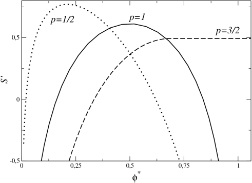
Figure 2: Entropy plot of $S^{\prime}\equiv S+(p+1)\log\rho$, where $S$ is the grand canonical entropy, as a function of reduced density $\phi^{*}$, for different values of parameter $p$. The three corresponding critical densities are $\phi^{*}_{c}=2/(3\pi)\simeq 0.212$ for $p=1/2$, $\phi^{*}=1/2$ for $p=1$ and $\phi^{*}_{c}=4(2/\pi)^{1/3}/5\simeq 0.688$ for $p=3/2$. In the first two cases no transition occurs. For $p>1$, the plateau seen for $\phi^{*}>\phi_{c}^{*}$ is a signature of the condensate formation. Note that for $p\leq 1$, the maximum allowed value of $\phi^{*}$ is 1, whereas one can have $\phi^{*}>1$ for $p>1$.

III.4 The case $p\leq 1$

Recall that, according to our model, for $p<1$ the volume of the $p$-sphere increases sub-linearly with its diameter and for $p=1$ the volume is equal to the diameter. Let us start by making the following observation. By definition, the inverse density is $1/{\rho}=L/N=(\sum_{i}x_{i})/N$. Due to the constraint $x_{i}\geq v_{i}^{1/p}$, it follows that $1/{\rho}\geq(\sum_{i}v_{i}^{1/p})/N$. For $p\leq 1$, one can use Jensen’s inequality to write

$$\frac{1}{\rho}\geq\frac{\sum_{i}v_{i}^{1/p}}{N}\geq\left[\frac{\sum_{i}v_{i}}{N}\right]^{1/p}=\phi^{1/p}.$$ (42)

Thus, for $p\leq 1$, one must necessarily have $\phi^{*}=\phi^{1/p}\rho\leq 1$. In other words, for a given $\rho$, one is physically allowed to increase $\phi$ only up to $\rho^{-p}$, i.e., $\phi\leq\rho^{-p}$.

Now, let us fix the density $\rho$ and imagine increasing $\phi$ from $0$ to its maximally allowed value $\rho^{-p}$. In other words, the reduced volume fraction $\phi^{*}=\phi^{1/p}\rho$ increases from $0$ to its maximally allowed value $1$. For a given $\phi^{*}$, we then have to solve (36) for $u=s/\lambda^{p}$.

The case $\bf{p<1}$: Consider first the case when $p<1$ strictly. The case $p=1$ will be discussed subsequently. For $p<1$, we notice that the integrals in (33) and (34) are convergent for any $u\in[-\infty,\infty]$. Their leading asymptotic behaviors can be easily deduced. Specifically, one finds that as $u\to\infty$

$$F_{\rho}(u) \to 1$$ (43)

$$F_{\phi}(u) \to \frac{1}{u}.$$ (44)

On the other hand, as $u\to-\infty$, to leading order,

$$F_{\rho}(u) \to |u|^{1/(1-p)}$$ (45)

$$F_{\phi}(u) \to |u|^{p/(1-p)}.$$ (46)

As a consequence, the function $\phi^{*}(u)$ in (36) has the following asymptotic behavior

$$\phi^{*}(u) \to 1\quad{\rm as}\quad u\to-\infty$$ (47)

$$\to u^{-1/p}\quad{\rm as}\quad u\to\infty.$$ (48)

In addition, one can check that $\phi^{*}(u)$ is a monotonically decreasing function of $u$, achieving its maximally allowed value $1$ as $u\to-\infty$ (see Fig. 3). Thus, for any given $\phi^{*}$, we can always find a solution $u$ to the equation $\phi^{*}=\phi^{*}(u)$ where $\phi^{*}(u)$ is given in (36). Knowing this solution $u$, one finds subsequently $\lambda>0$ from (31) and $s$ from the relation $s=u\,\lambda^{p}$. This means that the grand canonical framework works over the full allowed range $0\leq\phi^{*}\leq 1$ and the two marginals $p(v)$ and $p(x)$ have always the form in (18) and (19) with $\lambda$ and $s$ determined as above. This shows that there is no condensation for $p<1$.

Figure 3: The function $\phi^{*}(u)$ vs $u$ for $p=1/2$.

However, a vestige of the condensation transition still remains even for $p<1$. To see this, imagine again that we increase the value of the control parameter $\phi^{*}=\phi^{1/p}\rho$ from $0$ to $1$. As $\phi^{*}$ is increased, the solution $u$ to the equation (36) decreases monotonically from $\infty$ to $-\infty$ (see Fig. 3). Note that when the solution $u$ hits $0$, the corresponding value of $\phi^{*}(0)$ can be computed by putting $u=0$ in (36) and carrying out the elementary integrals that gives $F_{\rho}(0)=(p+1)$ and $F_{\phi}(0)=\Gamma(2p)/\Gamma(p)$. Thus

$$\phi^{*}(0)=\frac{1}{1+p}\,\left[\frac{\Gamma(2p)}{\Gamma(p)}\right]^{1/p}\;.$$ (49)

Now, let us investigate the entropy $S$ in (39) as a function of the control parameter $\phi^{*}$. As $\phi^{*}$ is increased monotonically from $0$ (and consequently $u$ decreases monotonically from $+\infty$), one can check that the entropy $S$, expressed as a function of $u$ as in (41), increases monotonically as long as $u>0$, i.e., $\phi^{*}<\phi^{*}(0)$ given in (49). For $\phi^{*}>\phi^{*}(0)$ (or $u<0$), the entropy decreases with increasing $\phi^{*}$. Thus, the entropy $S$ has a maximum value at $\phi^{*}=\phi^{*}(0)$, see Fig. 2. This is also evident from (40) where the derivative of the entropy as a function of $\phi$ (for fixed $\rho$) vanishes at $s=0$ and hence at $u=0$. Thus the value of $\phi$ at which the entropy becomes a maximum (for a fixed $\rho$) can be appropriately denoted by $\phi_{max}(\rho)$ and is given by

$$\phi_{max}(\rho)=\left[\frac{\phi^{*}(0)}{\rho}\right]^{p}=\frac{1}{\rho^{p}}\,\frac{1}{(1+p)^{p}}\,\frac{\Gamma(2p)}{\Gamma(p)}\;.$$ (50)

The corresponding maximum value of the entropy is obtained by putting $u=0$ in (41). Using $F_{\rho}(0)=(p+1)$ and $H(0)=\Gamma(p+1)$ from (29) we get

$$S_{max}=p+1+\ln\Gamma(p+1)-(p+1)\,\ln((p+1)\rho)\;.$$ (51)

Physically this means that for $\phi>\phi_{max}(\rho)$ or equivalently in terms of the reduced volume fraction, for $\phi^{*}>\phi^{*}(0)$, the configuration space becomes constrained resulting in the reduction of entropy.

Can one see a reflection of this vestige of a condensation transition directly in the volume distribution $p(v)$ in Eq. (18)? Indeed one does observe a change of behavior of $p(v)$ as the control parameter $\phi^{*}$ increases through $\phi_{\max}(\rho)$. As $\phi^{*}$ increases from $0$, the solution $u$ of $\phi^{*}(u)=u$ is positive as long as $\phi^{*}<\phi_{max}(\rho)$ (see Fig. 3). Consequently $s=u\lambda^{p}$ is also positive and hence the distribution $p(v)\propto\exp[-\lambda v^{1/p}-sv]$ is a monotonically decreasing function of $v$ with its maximum at $v=0$. However, when $\phi^{*}>\phi_{max}(\rho)$, the solution $u$ and hence $s$ becomes negative. As a result, $p(v)\propto\exp[-\lambda v^{1/p}+|s|v]$ now develops a maximum at a nonzero characteristic volume $v^{*}=(p|s|/\lambda)^{p/(1-p)}$.

The case $\bf{p=1}$: The general conclusion reached above for $p<1$ remains valid even for the marginal case $p=1$, though the details are slightly different. Indeed, for $p=1$, we can obtain explicit solutions for the marginal distributions. To see this, let us first explicitly express $\lambda$ and $s$ in terms of $\rho$ and $\phi$. The integrals in (33) and (34) can be easily performed explicitly for $p=1$ giving

$$F_{\rho}(u)=\frac{u+2}{u+1}\;;\quad F_{\phi}(u)=\frac{1}{u+1}.$$ (52)

Thus, unlike the $p<1$ case where the allowed range of $u$ was $u\in[-\infty,\infty]$, for $p=1$, $u$ has the allowed range $u\in[-1,\infty]$. Eq. (36) then gives

$$\phi^{*}(u)=\frac{1}{u+2}.$$ (53)

Thus $\phi^{*}(u)$ is again a monotonically decreasing function of $u$ in $u\in[-1,\infty]$ and for any given $\phi^{*}$ one can always find a solution $u=1/\phi^{*}-2$. Hence, as in the case $p<1$, there is no condensation for $p=1$ as well.

Note that at $u=0$, $\phi^{*}(0)=1/2$ and hence $\phi_{max}(\rho)=1/(2\rho)$. Also, (31) and (32) yield explicitly

$$\phi=\frac{1}{s+\lambda}$$ (54)

$$\frac{1}{\rho}-\phi=\frac{1}{\lambda}\;,$$ (55)

determining $\lambda=\rho/(1-\rho\phi)$ and $s=(1-2\rho\phi)/(1-\rho\phi)$ in terms of $\rho$ and $\phi$. This also gives, using (24), $\eta=\rho\phi=\phi^{*}$. The grand canonical joint distribution for the separation and volume of a particle (17) is

$$p(x,v)=\lambda(s+\lambda)e^{-x\lambda-vs}\theta(x-v)\;.$$ (56)

The marginal distributions (18,19) become

$$p(v) = \frac{{\rm e}^{-v/\phi}}{\phi}$$ (57)

$$p(x) = \frac{\rho}{1-2\,\rho\,\phi}\left[{\rm e}^{-{\rho\,x}/(1-\rho\,\phi)}-{\rm e}^{-x/\phi}\right]\;.$$ (58)

Thus, although there is no phase transition for $p=1$, there is a change in the leading behaviour of $p(x)$ as the volume per particle $\phi$ is increased past $\phi_{max}(\rho)=1/(2\rho)$: for $\phi<1/(2\rho)$ the large $x$ behaviour is $p(x)\simeq{\rm e}^{-x\rho/(1-\rho\,\phi)}\rho/(1-2\,\rho\,\phi)$; for $\phi=1/(2\rho)$ the large $x$ behaviour is $p(x)=x{\rm e}^{-x/\phi}/\phi^{2}$ (note that this expression, for $\phi=1/(2\rho)$, holds for all values of left-to-left distances $x$); for $\phi>1/(2\rho)$ the large $x$ behaviour is $p(x)\simeq{\rm e}^{-x/\phi}\rho/(2\,\phi\,\rho-1)$. Thus for $\phi>1/(2\rho)$, the exponential decay of $p(x)$ is the same as that of $p(v)$.

The entropy per particle (39) reads

$$S=\ln(1-\rho\phi)-\ln\rho+\ln\phi+2.$$ (59)

Note that, as mentioned below (39), the entropy $S$ is not restricted to be only positive. This is evident in the $p=1$ case from (59) where $S$ can be negative for certain values of the parameters $\rho$ and $\phi$. One can verify easily that the entropy $S$ in (59) has a maximum at $\phi=\phi_{max}(\rho)=1/(2\rho)$ with value $S_{\max}=2+\ln(2)-2\ln(2\rho)$ from (51), see also Fig. 2. As $\phi$ increases past $1/(2\rho)$ the entropy decreases, implying a constrained configuration space. Thus the scenario for $p=1$ case is similar to $p<1$ discussed earlier, as seen clearly in Fig. 2 for the two representative cases $p=1/2$ and $p=1$.

III.5 The case p$>$1

For $p>1$, the integrals on the right hand side of (33) and (34) are convergent only for $u>0$. Thus the lowest allowed value of $u$ is $0$. When $u\to 0$, the function $\phi^{*}(u)$ in (36) approaches $\phi^{*}(0)$ which is still given exactly by (49). Thus this is the maximum value of $\phi^{*}$ allowed by the grand canonical ensemble. If $\phi^{*}$ exceeds $\phi^{*}(0)$, $u=s/\lambda^{p}$ cannot decrease below $0$. It then sticks to its value $u=0$ and all the extra volume condenses into a single site. Thus $\phi^{*}(0)$ is the critical value beyond which the grand canonical ensemble breaks down signalling the onset of a condensation transition.

At this critical point, the volume fraction $\phi=[\phi^{*}(0)/\rho]^{p}$ will again be denoted by $\phi_{max}(\rho)$ and has the same expression as in the $p\leq 1$ case, namely

$$\phi_{max}(\rho)=\frac{1}{\rho^{p}}\,\frac{1}{(1+p)^{p}}\,\frac{\Gamma(2p)}{\Gamma(p)}\;.$$ (60)

Also, letting $u=0$ in (31) gives the critical value $\lambda_{c}=(p+1)\rho$. Consequently, the two marginals in (18) and (19) at the critical point become

$$p(v) \to \left[G(0,\lambda)\right]^{-1}\frac{1}{\lambda}{\rm e}^{-\lambda v^{1/p}}=\frac{1}{\Gamma(1+p)}\,\left[\rho\,(1+p)\right]^{p}{\rm e}^{-\rho\,(1+p)\,v^{1/p}}$$ (61)

$$p(x) \to \left[G(0,\lambda)\right]^{-1}{\rm e}^{-\lambda x}x^{p}=\frac{1}{\Gamma(1+p)}\,\left[\rho\,(1+p)\right]^{1+p}\,x^{p}\,{\rm e}^{-\rho\,(1+p)\,x}$$ (62)

Thus at condensation $p(v)$ changes from (dominant) exponential decay (18) to a slower stretched exponential decay (61) and $p(x)$ changes from an exponential decay (19) to the exponential decay multiplied by $x^{p}$ (62). We interpret these results as describing the critical fluid; in the condensed phase we expect a condensate to coexist with the critical fluid. For later purposes, we also note that at the critical point the dimensionless line coverage

$$\eta\to\eta_{c}=\frac{p}{(1+p)}$$ (63)

which follows by substituting $\lambda_{c}=(p+1)\rho$ in (26).

How does the entropy $S$ behave as $\phi$ increases from $0$ to $\phi_{max}(\rho)$ for fixed $\rho$? As $\phi$ increases monotonically, $u$ decreases monotonically till $u$ hits $0$. Consequently, the entropy $S$ in (41) increases monotonically up to $u=0$, achieving a maximum value at $u=0$ (or equivalently at $\phi=\phi_{max}(\rho)$) given by the same expression as in the case $p\leq 1$ in (51) namely,

$$S_{max}=p+1+\ln\Gamma(p+1)-(p+1)\,\ln((p+1)\rho)).$$ (64)

What happens to the entropy when $\phi$ exceeds the critical value $\phi_{\max}(\rho)$, i.e., when a condensate sets in? To see this, we note that $\phi_{max}(\rho)$ in (60) can be neatly expressed in terms of the $p$-th moment $\langle x^{p}\rangle$ of the critical marginal $p(x)$ in (62). This moment can be easily computed and comparing to the expression of $\phi_{max}(\rho)$ in (60) one easily verifies that

$$\phi_{max}(\rho)=\frac{1}{2}\langle x^{p}\rangle\;.$$ (65)

The physical meaning of (65) is that condensation occurs when the volume per particle is equal to half the mean available volume per particle in the grand canonical distribution. In the case $p\leq 1$ this is the value of $\phi$ above which the entropy decreases. For $p>1$, the intuitive explanation is that at this point, rather than the entropy decreasing as was the case for $p=1$, the entropy can be held constant by one particle containing the excess volume and leaving the rest of the system at the critical volume fraction, see Fig. 2.

Let us then summarize the $p>1$ case. The existence of the grand canonical solution means that the system is in a fluid state. Thus, for fixed $\rho$, $\phi_{\max}(\rho)$ in (60) is precisely the critical line in the $(\rho,\phi)$ phase diagram, as shown in Fig. (4) for $p=2$. When the volume fraction $\phi$ exceeds this critical value $\phi_{\max}(\rho)$, the grand canonical description breaks down and a condensate forms in the system. The entropy $S$ increases monotonically with increasing $\phi$ till $\phi$ hits the critical value $\phi_{max}(\rho)$ where it achieves its maximum value $S_{max}$ given in (64). When $\phi$ is increased to a value $\phi>\phi_{max}(\rho)$, the entropy remains at the maximal value through one particle containing the excess volume and forming a condensate.

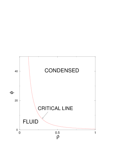
Figure 4: Phase diagram in the $(\rho,\phi)$ plane for $p=2$. The critical line $\phi_{max}(\rho)=\frac{2}{3\,\rho^{2}}$ (for $p=2$) separates the fluid and the condensed phase.

III.6 The large p limit

The limit $p\to\infty$ is worth mentioning also as it makes links with some other well studied problems. As mentioned in the begining of Section 2, in the $p\to\infty$ limit our polydisperse hard-rod system reduces to the classical monodisperse Tonks gas of hard rods where each rod has the same size $1$. In this case, our result for the gap distribution in (27) (valid for general $p$), reduces to that of the classical Tonks gas.

On the other hand (again for $p\to\infty$), the volume of each rod becomes a “passive” property (a color $v\in[0,\infty[)$. From (18), this property is exponentially distributed ($p(v)\propto\exp(-sv)$). Such a Poissonian distribution may have been anticipated, and is readily obtained within the free energy functional formalism presented in section V. We note that this exactly coincides with the exponential distribution of wealth and income obtained in the model presented in reference Dragu .

We also note that in the large $p$ limit, the condensation transition disappears. Thus the system is always in a fluid state and the volume statistics obey “ideal gas” behaviour. In the hard core language of section V, we will indeed see that the critical line fraction tends to unity for large $p$, so that the parameter range $\phi>\phi_{max}$ actually corresponds to an unphysical region where “hard rods” necessarily overlap. Hence, the model of Ref Dragu shows no condensation transition (more complex interactions between the “agents” would be required).

IV Micro-canonical Analysis of the Condensed Phase for $p>1$

For $p>1$ the grand canonical ensemble can only support a volume per particle $\phi\leq\phi_{max}(\rho)$, therefore in order to fully analyse the condensed phase, where $\phi=V/N>\phi_{max}(\rho)$, one needs to work within the micro-canonical ensemble.

To compute the micro-canonical partition function one inverts the Laplace transforms in (15)

$$Z_{N}(L,V) = \int_{c_{1}-i\infty}^{c_{1}+\infty}\frac{{\rm d}s}{2\pi i}\int_{c_{2}-i\infty}^{c_{2}+\infty}\frac{{\rm d}\lambda}{2\pi i}{\rm e}^{sV+\lambda L}{\cal Z}_{N}(\lambda,s)$$ (66)

where $c_{1}$ and $c_{2}$ are chosen so that the integration contours are to the right of any singularities. Using the expression (15) one finds

$$Z_{N}(L,V) = \int_{c_{1}-i\infty}^{c_{1}+\infty}\frac{{\rm d}s}{2\pi i}\int_{c_{2}-i\infty}^{c_{2}+\infty}\frac{{\rm d}\lambda}{2\pi i}{\rm e}^{N\psi(\lambda,s)}$$ (67)

where

$$\psi(\lambda,s)=\frac{\lambda}{\rho}+s\phi-\ln\lambda+\ln\left[\int_{0}^{\infty}{\rm d}v\ {\rm e}^{-sv-\lambda v^{1/p}}\right]\;.$$ (68)

The integral (67) may be evaluated by the saddle-point method. The saddle-point equations coming from the conditions $\frac{\partial\psi}{\partial\lambda}=0$ and $\frac{\partial\psi}{\partial s}=0$ read

$$\frac{1}{\rho} = \frac{1}{\lambda}+\frac{\int_{0}^{\infty}{\rm d}v\,v^{1/p}{\rm e}^{-sv-\lambda v^{1/p}}}{\int_{0}^{\infty}{\rm d}v\ {\rm e}^{-sv-\lambda v^{1/p}}}$$ (69)

$$\phi = \frac{\int_{0}^{\infty}{\rm d}v\,v{\rm e}^{-sv-\lambda v^{1/p}}}{\int_{0}^{\infty}{\rm d}v\ {\rm e}^{-sv-\lambda v^{1/p}}}$$ (70)

which are, of course, precisely the grand canonical equations (31, 32). Thus when the saddle point exists (i.e. in the fluid phase) the results of the grand canonical and micro-canonical ensembles coincide. However, in the condensed phase $\phi>\phi_{max}(\rho)$ one can no longer solve the saddle-point equations for $s\geq 0$. Therefore $Z_{N}(L,V)$ must be evaluated by an alternative approach.

It will be useful to consider the Laplace transform of $Z_{N}(L,V)$ with respect to the length $L$ (rather than the double Laplace transform of $Z_{N}(L,V)$ which generates the grand canonical partition function).

$${\widetilde{Z}}_{N}(\lambda,V) = \int_{0}^{\infty}{\rm d}L\ {\rm e}^{-\lambda L}Z_{N}(L,V)$$ (71)

$$= \prod_{i=1}^{N}\int_{0}^{\infty}{\rm d}v_{i}\int_{v_{i}^{1/p}}^{\infty}{\rm d}x_{i}\ {\rm e}^{-\lambda x_{i}}\delta(\sum_{i}v_{i}-V)$$ (72)

$$= \left[\frac{\int_{0}^{\infty}{\rm d}w{\rm e}^{-\lambda w^{1/p}}}{\lambda}\right]^{N}\left[\prod_{i=1}^{N}\int_{0}^{\infty}{\rm d}v_{i}f(v_{i})\right]\delta(\sum_{i}v_{i}-V)$$ (73)

where we have defined

$$f(v_{i})=\frac{{\rm e}^{-\lambda v_{i}^{1/p}}}{\int_{0}^{\infty}{\rm d}w\ {\rm e}^{-\lambda w^{1/p}}}.$$ (74)

This definition ensures that the integral of $f(v_{i})$ is normalised to unity therefore $f(v_{i})$ may be considered as the probability distribution for a positive random variable $v_{i}$. Then the quantity

$$\Omega_{N}(\lambda)=\left[\prod_{i=1}^{N}\int_{0}^{\infty}{\rm d}v_{i}f(v_{i})\right]\delta(\sum_{i}v_{i}-V)\;,$$ (75)

manifest in (73), is the probability that a sum of $N$ independent positive random variables each distributed according to $f$ is equal to $V$. Assuming that $f$ has finite first and second moments $\mu_{1}$ and $\mu_{2}$, as it does in the case (74), where

$$\mu_{n}=\int_{0}^{\infty}{\rm d}v\ v^{n}f(v)\;,$$ (76)

one can invoke some limiting results on the sum of a large number $N$ of such random variables. We first define

$$V_{c}=N\mu_{1}$$ (77)

then the following results for sums of random variables derived in a different context EMZ06 will be useful

$$\mbox{For}\quad V-V_{c}\sim O(N^{2/3})\qquad\Omega_{N}(\lambda,V)\simeq\frac{1}{\sqrt{2\pi N\Delta^{2}}}{\rm e}^{-\frac{(V-V_{c})^{2}}{2N\Delta^{2}}}$$ (78)

$$\mbox{For}\quad V>V_{c}\quad\mbox{and}\quad V-V_{c}\sim O(N)\qquad\Omega_{N}(\lambda,V)\simeq Nf(V-V_{c})$$ (79)

where $\Delta^{2}=\mu_{2}-\mu_{1}^{2}$. The first result is a central limit theorem which expresses the fact that the sum is Gaussian distributed about the mean $V_{c}$. The second is a large deviation result whose interpretation is that for the sum of random variables to be equal to a value $V$, much greater than the mean $V_{c}$, one of the random variables should be equal to $V-V_{c}$ to leading order and the other $N-1$ should be of $O(\mu_{1})$. In (79) the factor $f(V-V_{c})$ comes from the probability of the large random variable and the factor $N$ comes from the number of ways of choosing the large contribution from the $N$ random variables.

Let us note that $\mu_{1}$ is precisely the critical volume fraction $\phi_{max}(\rho)$ defined in the previous section. This follows by computing the first moment of $f(v)$ in (74) and comparing it to the expression of $\phi_{\max}(\rho)$ in (60). Thus

$$V_{c}=N\mu_{1}=N\phi_{max}(\rho)$$ (80)

justifying the subscript $c$ (critical) for the volume $V$.

We may now obtain forms for $Z_{N}(L,V)$ near to criticality and in the condensed phase by inverting the Laplace transform

$$Z_{N}(L,V) = \int_{c_{1}-i\infty}^{c_{1}+i\infty}\frac{\rm d\lambda}{2\pi i}{\rm e}^{L\lambda}\left[\frac{\int_{0}^{\infty}{\rm d}w\ {\rm e}^{-\lambda w^{1/p}}}{\lambda}\right]^{N}\Omega_{N}(\lambda,V)\;.$$ (81)

Here the $\lambda$ integral may be evaluated without problem using the saddle-point method with the saddle located (to leading order for large $L$, large $N$ but keeping the ratio $\rho=N/L$ fixed) at $\lambda_{*}=(p+1)\rho$. For $\Omega_{N}(\lambda^{*},V)$ one can use the results in (78) and (79). This gives

$$Z_{N}(L,V)\simeq\left(\frac{N}{2\pi(p+1)}\right)^{1/2}{\rm e}^{L\lambda_{*}}\left[\frac{p\Gamma(p)}{(\lambda_{*})^{p+1}}\right]^{N-1}\quad\mbox{for}\quad V-V_{c}\sim O(N)$$ (82)

$$Z_{N}(L,V)\simeq\left(\frac{\lambda_{*}^{2}}{2\pi(p+1)N}\right)^{1/2}{\rm e}^{L\lambda_{*}}\left[\frac{p\Gamma(p)}{(\lambda_{*})^{p+1}}\right]^{N}\frac{{\rm e}^{-\frac{(V-V_{c})^{2}}{2N\Delta^{2}}}}{\sqrt{2\pi N\Delta^{2}}}\quad\mbox{for}\quad V-V_{c}\sim O(N^{2/3})$$

Therefore for $\phi\geq\phi_{max}(\rho)$ the entropy per particle, given in the micro-canonical ensemble by

$$S=\frac{1}{N}\ln Z_{N}(L,V)\;,$$ (84)

remains fixed at

$$S=p+1+\ln\Gamma(p+1)-(p+1)\ln\left((p+1)\rho\right)\;.$$ (85)

Note that this is precisely the maximal value $S_{\max}$ in (64) computed in the fluid state. To summarize, for $p>1$, the entropy $S$ increases monotonically with increasing $\phi$, achieves its maximal value $S_{max}$ at $\phi=\phi_{\max}(\rho)$ and then remains fixed at this value for all $\phi>\phi_{max}(\rho)$.

We may also consider the marginal distribution $p(v)$ in the condensed phase. As a signature of condensation this distribution should contain a bump at $v=V-V_{c}$. In the micro-canonical ensemble we have

$$p(x,v)=\frac{Z_{N-1}(L-x,V-v)}{Z_{N}(L,V)}\theta(x-v^{1/p})$$ (86)

Integrating out $x$ yields

$$p(v)=Z_{N}(L,V)^{-1}\int_{v^{1/p}}^{L}{\rm d}x\ Z_{N-1}(L-x,V-v)$$ (87)

One can then substitute the asymptotic behavior of the function $Z_{N}(L,V)$ obtained in (82) and (IV) to estimate $p(v)$ in (87). Omitting details, we find that

$$\mbox{For}\quad v\ll V-V_{c}\quad p(v)\simeq\frac{\lambda^{p}_{*}}{\Gamma(1+p)}{\rm e}^{-\lambda_{*}v^{1/p}}$$ (88)

$$\mbox{For}\quad v=V-V_{c}+O(N^{2/3})\quad p(v)\simeq\frac{1}{N}\frac{1}{\sqrt{2\pi N\Delta^{2}}}{\rm e}^{-\frac{(v-(V-V_{c}))^{2}}{2N\Delta^{2}}}$$ (89)

The latter piece (89) of $p(v)$ represents the condensate: it has a total weight $1/N$ signifying a single condensate site and shows a Gaussian distribution of the bump around the excess volume $V-V_{c}$.

V The free energy functional route

Having established that our problem, defined in terms of dynamical rules, admits a factorized steady state probability with detailed balance, we can envisage the steady state as the equilibrium state of a hard-rod model, where the distribution of rod lengths $\ell\equiv v^{1/p}$ is not known a priori. This size distribution should be that which minimizes the free energy of the system (or equivalently maximizes the total entropy, since we only deal here with excluded volume interactions). Our goal in the remainder is therefore to provide a different, perhaps more physical –but fully equivalent– perspective, and obtain the optimal polydispersity minimizing the free energy functional of a hard-rod system, with the same global constraints as in section II: fixed density $\rho=N/L$, and fixed $p$-moment of the length distribution ($\langle v\rangle=\langle\ell^{p}\rangle$), where $p$ is a parameter of the model, and is fixed as in previous sections. In doing so, we are only interested here in the size distribution (variable $v$), and not in the joint distribution of size and gap $x$. In this respect, the approach of sections III and IV provides more detailed information.

The problem we face is the one-dimensional analogue of the optimal packing of polydisperse hard sphere fluids addressed in Refs. ZBTCF99 ; B00 ; BC01 , which exhibits an unexpected condensation transition. The free energy functional approach put forward here is akin to that used in ZBTCF99 , with nevertheless the interesting feature that in the present 1D geometry, exact results can be obtained. On the other hand, approximations of Percus-Yevick type or more involved treatments were necessary in Refs ZBTCF99 ; B00 ; BC01 . Indeed, the problem boils down to finding the size dependence of the chemical potential of a given species in a polydisperse mixture, which is not known exactly for hard discs or hard spheres.

V.1 Free energy functional for polydisperse hard rods

We work in the canonical ensemble where a distribution of $N$ hard rods at temperature $T$ occupies an available length $L$. Their total length is denoted $L_{p}$ and defines the line coverage (or packing fraction) $\eta=L_{p}/L=\rho\langle\ell\rangle$ where $\rho=N/L$ is the density and $\langle\ell\rangle$ is the mean size. To establish the connection with the $p$-spheres discussed earlier, we can view each rod of size $\ell$ as a (hyper)sphere constrained to move on a line, and having “volume” $v=\ell^{p}$.

Writing the ideal entropy of a multicomponent and discrete system is straightforward SS82 , but the limit of a continuous distribution requires some care (see the discussion below). For hard rods, the free energy functional may be written as a sum of ideal and excess contributions TheOtherEvans :

$$\beta{\cal F}\{W\}=N\,\int{\rm d}\ell\,W(\ell)\left[\ln\left(\Lambda^{2}\rho W(\ell)j_{\ell}(\ell)\right)-1\right]+\beta{\cal F}_{\hbox{\scriptsize ex}}\{W\}.$$ (90)

where $\Lambda$ is an irrelevant length scale, $\beta$ is the inverse temperature, and $W$ is the length probability distribution function (such that $\int d\ell\ \ell W(\ell)=\langle\ell\rangle$). The excess free energy for a homogeneous system of hard rods is known exactly, $\beta{\cal F}_{\hbox{\scriptsize ex}}\{W\}=-\ln(1-\eta)$  SS82 , and can be generalized to inhomogeneous situations TheOtherEvans . In Eq.( 90), the function $j_{\ell}(\ell)$ –yet to be specified– ensures that different choices for the labelling of the particles will lead to the same optimal length distribution $W(\ell)$. One could indeed choose $v=\ell^{p}$ (or say any other power) as a working variable, with an associated “labelling” function $j_{v}(v)$ and a probability distribution function $W_{v}$ such that $W(\ell)=p\,\ell^{p-1}W_{v}(\ell^{p})$. Enforcing the consistency of both descriptions imposes $j_{\ell}(\ell)=\ell^{p-1}j_{v}(\ell^{p})$ (up to an irrelevant prefactor), where the factor $\ell^{p-1}$ is the Jacobian of the transformation $\ell\to\ell^{p}$. The natural labelling for the particles, i.e. that which gives a constant function $j$, follows from the way polydispersity is sampled (see e.g. ZBTCF99 ; B00 ), and reflects the dynamics of the system. In the following Monte Carlo simulations, we will attempt to change the size of two particles $\ell_{1}$ and $\ell_{2}$ selected at random by adding a small increment to $\ell_{1}^{p}$ and conversely subtracting the same quantity from $\ell_{2}^{p}$, in accordance with the rule specified in section II and more precisely with the requirement that $b(v)=1$. This corresponds to a flat function $j_{v}$, and hence to $j_{\ell}=\ell^{p-1}$. However, given an arbitrary $b(v)$ (not constant) in the microscopic rate in Eq. (9), it is far from evident how to choose an appropriate labelling function $j_{v}(v)$ in the macroscopic description in Eq. (90), that would precisely correspond to this microscopic rate.

Minimization of ${\cal F}$—with the two constraints of normalization $\int{\rm d}\ell W(\ell)=1$ and fixed $p$-moment $\int{\rm d}\ell\ell^{p}W(\ell)$, that can be included by two Lagrange multipliers—leads to the functional form of the optimal size distribution $W^{*}$, which should then coincide with the probability distribution function of $v^{1/p}$, where the statistics of $v$ is given by Eq. (18). Since the explicit expression of $\cal F$ is known, see above, this provides a first angle of attack to our problem. However, interesting information follows from more microscopic considerations and scaling arguments, as becomes clear below. Note that the constraint that the line coverage should not exceed unity is not explicitly considered, but is implicitly encoded in the excess contribution to the free energy functional (90).

V.2 Optimal polydispersity distribution

We take advantage of the fact that any infinitesimal change in $W^{*}$ has a vanishing free energy cost $\delta{\cal F}$, provided the two aforementioned constraints are satisfied. We proceed in two steps: a) a given rod of arbitrary length $\ell_{0}$ is expanded : $\ell_{0}\to\ell_{0}+\delta\ell_{0}$; b) all particles are rescaled ($\ell\to\alpha\,\ell$) in order to fulfil the constraint of a conserved $p$-th moment. In the first step, this moment changes by an amount

$$\frac{1}{N}\,\left[(\ell_{0}+\delta\ell_{0})^{p}-\ell_{0}^{p}\right]\,\simeq\,\frac{1}{N}\,p\,\ell_{0}^{p-1}\,\delta\ell_{0}$$ (91)

while in the second stage, it changes by $(\alpha^{p}-1)\langle\ell^{p}\rangle\simeq p(\alpha-1)\langle\ell^{p}\rangle$. Enforcing the conservation of $\langle\ell^{p}\rangle$ then imposes

$$\alpha\,\simeq\,1-\frac{\ell_{0}^{p-1}\delta\ell_{0}}{N\langle\ell^{p}\rangle}$$ (92)

In stages a)+b), the distribution function changes by an amount

$$\delta W=\frac{1}{N}\,\left[\,\delta\left(\ell-\ell_{0}-\delta\ell_{0}\right)\,-\,\delta\left(\ell-\ell_{0}\right)\,\right]+(1-\alpha)\,\frac{{\rm d}[\ell W]}{{\rm d}\ell}.$$ (93)

It proves convenient to express the variation of the ideal part of the free energy in terms of the probability distribution function $W_{v}$ of $v$. This yields, with $v_{0}=\ell_{0}^{p}$

$$\delta{\cal F}_{\hbox{\scriptsize id}}=k_{B}T\left\{\frac{W_{v}^{\prime}(v_{0})}{W_{v}(v_{0})}+\frac{1}{\langle v\rangle}\right\}\delta v_{0}.$$ (94)

The excess contribution variation –which is most conveniently expressed in terms of $\ell$ rather than $v$– is in addition exactly the reversible work required to perform the changes under consideration. In step a), we note that this work is the same as if a confining “wall” would be displaced a distance $\delta\ell_{0}$ thereby compressing the system. We therefore have

$$\delta{\cal F}_{a}\,=\,P\,\delta\ell_{0},$$ (95)

where $P$ is the pressure of the system. This relation is specific to the one dimensional case, and at the root of important simplifications as compared to higher dimensions TP08 . On the other hand, it is a general result that in any space dimension, the work performed during step b) is (see e.g. appendix B of ZBTCF99 )

$$\delta{\cal F}_{b}\,=\,-\frac{P_{\hbox{\scriptsize ex}}}{\eta}\delta L_{p}$$ (96)

where $P_{\hbox{\scriptsize ex}}=P-\rho kT$ is the excess pressure and $\delta L_{p}$ is the total volume change of the particle upon the rescaling $\ell\to\alpha\,\ell$: $\delta L_{p}=(\alpha-1)L_{p}=(\alpha-1)N\langle\ell\rangle$. Making use of Eq. (92), we finally have :

$$\frac{\delta{\cal F}_{\hbox{\scriptsize ex}}}{\delta\ell_{0}}=P-\frac{P_{\hbox{\scriptsize ex}}}{\eta}\,\frac{\ell_{0}^{p-1}\langle\ell\rangle}{\langle\ell^{p}\rangle}.$$ (97)

Combining this with Eq. (94) supplemented by the requirement that $\delta{\cal F}=0$ for $W=W^{*}$ (or equivalently $W_{v}=W_{v}^{*}$) gives

$$\frac{{W_{v}^{*}}^{\prime}(v_{0})}{W_{v}^{*}(v_{0})}+\frac{1}{\langle v\rangle}+\frac{P}{p}\,v_{0}^{1/p-1}-\frac{P_{\hbox{\scriptsize ex}}}{\eta}\,\frac{\langle\ell\rangle}{p\,\langle\ell^{p}\rangle}=0.$$ (98)

After integration with respect to $v_{0}$, we arrive at

$$W_{v}^{*}(v)\,\propto\,\exp\left\{-\beta Pv^{1/p}\,+\,\left(\frac{\beta P_{\hbox{\scriptsize ex}}\langle\ell\rangle}{p\,\eta}-1\right)\,\frac{v}{\langle\ell^{p}\rangle}\right\}.$$ (99)

This is, expectedly, the very same form as obtained in section III, see Eq. (18). In addition, Eq. (99) above makes explicit the connection between the chemical potentials $\lambda$ and $s$ appearing in Eq. (18) and intensive thermodynamic quantities, for example $\lambda=\beta P$, see Eq. (26). Equivalently, in terms of the $\ell$ variable, we obtain

$$W^{*}(\ell)\,=\,{\cal A}\,\ell^{p-1}\,\exp\left\{-\beta P\ell\,+\,\left(\frac{\beta P_{\hbox{\scriptsize ex}}\langle\ell\rangle}{p\,\eta}-1\right)\,\frac{\ell^{p}}{\langle\ell^{p}\rangle}\right\}$$ (100)

where ${\cal A}$ is a normalization factor. As alluded to earlier, it is noteworthy here that the pressure is exactly related to the density $\rho$ through Tonks ; SS82 ; TP08

$$\beta P\,=\,\frac{\rho}{1-\eta}\qquad\hbox{where}\quad\eta=\rho\,\langle\ell\rangle.$$ (101)

One can note that the low density behaviour of $W^{*}$ allows for some consistency test of our prediction. When the density vanishes, one has $P\to 0$ and $\beta P_{\hbox{\scriptsize ex}}/\eta\to 0$, so that

$$W^{*}(\ell)\,\propto\,\ell^{p-1}\exp\left(-\frac{\ell^{p}}{\langle\ell^{p}\rangle}\right),$$ (102)

hence an exponential distribution of $v=\ell^{p}$ (the conserved quantity). Such an expression also immediately follows from direct minimization of the functional (90), restricted to its ideal contribution (${\cal F}_{\hbox{\scriptsize ex}}=0$). We recover here the expression obtained in section III in the large $p$ limit. As mentioned earlier, we also recover the results reported in an econophysics context Dragu for a simple model where agents act as our ideal particles, exchanging random amounts of a quantity $v$ (money) in binary encounters.

With a weight function such as (102), one immediately finds

$$\frac{\int_{0}^{\infty}\ell^{p}\,W^{*}(\ell)\,{\rm d}\ell}{\int_{0}^{\infty}W^{*}(\ell)\,{\rm d}\ell}=\langle\ell^{p}\rangle,$$ (103)

as it should (the quantity $\langle\ell^{p}\rangle$ appearing on the l.h.s. of (102) is therefore indeed the moment of order $p$ of the distribution). This shows the consistency of our distribution function in the low density limit. The corresponding mean size follows, assuming again the low density form (102) :

$$\frac{\int_{0}^{\infty}\ell\,W^{*}(\ell)\,{\rm d}\ell}{\int_{0}^{\infty}W^{*}(\ell)\,{\rm d}\ell}=\Gamma(1+1/p)\,\,\langle\ell^{p}\rangle^{1/p},$$ (104)

With the standard “functional route” alluded to earlier (i.e. direct minimization of Eq.(90)) which does not provide explicitly Lagrange multipliers, the requirement (103) together with normalization would determine those multipliers for any density.

In the remainder, the star superscript will be omitted to refer to the optimal distribution $W^{*}$, without ambiguity.

V.3 The condensation transition

We revisit here the condensation transition brought to the fore in section 3, in the more liquid-state language of hard rods. Since the excess pressure following from (101) fulfils the identity $P_{\hbox{\scriptsize ex}}/\eta=P$, as can be readily checked, the distribution (100) can be rewritten more explicitly as

$$W(\ell)\,=\,{\cal A}\,\ell^{p-1}\,\exp\left[-\frac{\rho\ell}{1-\eta}\,+\,\left(\frac{\eta-\eta_{c}}{\eta_{c}(1-\eta)}\right)\,\frac{\ell^{p}}{\langle\ell^{p}\rangle}\right],$$ (105)

with $\eta_{c}=p/(1+p)$. For $p\leq 1$, this distribution is normalizable for all line coverages $\eta$ (given that $\eta<1$). This is no longer the case for $p>1$, provided that $\eta>\eta_{c}$, where $\eta_{c}$ will be referred to as the critical line coverage. For $p>1$ and $\eta>\eta_{c}$, the divergent behaviour of distribution (105) at large $\ell$ is indicative of the formation of a macroscopic aggregate with size $L_{0}$. The scenario is identical to that inferred from the observations of Ref. ZBTCF99 and worked out in BC01 . The system relaxes by transferring “volume” to the aggregate, which effectively acts as a piston and coexists with a polydisperse mixture ${\cal M}$ confined in a region of size $L-L_{0}$. In this region, the size distribution obeys Eq. (105), where $\eta$ is no longer the total line coverage fraction, but should be replaced by the line coverage $\eta_{{}_{\cal M}}$ in the region free of aggregate. The different line coverages in the problem are connected through

$$\eta_{{}_{\cal M}}=\frac{\eta-\eta_{0}}{1-\eta_{0}},$$ (106)

where $\eta_{0}=L_{0}/L$ is the line coverage of the aggregate. We show in Appendix B that

$$\eta_{0}=\left\{\begin{array}[]{c l}0&\hbox{ for }\eta<\eta_{c}\\ \displaystyle\frac{\eta-\eta_{c}}{1-\eta_{c}}&\hbox{ for }\eta>\eta_{c}.\end{array}\right.$$ (107)

The line coverage $\eta_{0}$ may be considered as an order parameter for the transition. The key ingredient to arrive at Eq. (107) is that the fluid outside the condensate (assuming the latter species forms) is critical, in the available length $L-L_{0}$. It therefore has line coverage $\eta_{\cal M}=\eta_{c}$, and size distribution

$$W(\ell)\,\propto\,\ell^{p-1}\,\exp\left[-\frac{\rho\ell}{1-\eta_{c}}\right].$$ (108)

We note finally that the case $p\to\infty$ is specific in that we then have $\eta_{c}\to 1$ (while $\phi^{*}_{c}\to 4/e$). Since the hard core constraint imposes $\eta<1$, we see here why the large $p$ limit reduces in fact to the ideal gas case, where $\ell^{p}$ is exponentially distributed and no transition occurs.

VI Comparison with simulation results

In order to verify analytical predictions it is useful to compare with numerical results. For example, numerical studies of condensation have in the past revealed important information about when the asymptotic behaviour predicted analytically actually emerges in a finite system.

VI.1 Control parameter and critical point

To analyze in more detail the scenario at work and put our predictions to the test, we perform Monte Carlo simulations. We first have to introduce a relevant control parameter (we emphasize that except when $p=1$, the line coverage or packing fraction $\eta$ (24) is not a conserved quantity, but is self-consistently determined). Since both the density and $\langle\ell^{p}\rangle$ are conserved variables, we will use the dimensionless reduced volume fraction

$$\phi^{*}\,=\,\rho\langle\ell^{p}\rangle^{1/p},$$ (109)

introduced in eq. (35). A simple convexity argument shows that for $p>1$, $\phi^{*}>\eta$, while the reverse holds for $p<1$. Having chosen $\langle\ell^{p}\rangle^{1/p}$ as our relevant length scale, we also introduce a reduced pressure

$$P^{*}\,\equiv\,\beta P\langle\ell^{p}\rangle^{1/p}=\frac{\phi^{*}}{1-\eta}=\frac{\phi^{*}}{1-\rho\langle\ell\rangle},$$ (110)

and a rescaled length

$$\widetilde{\ell}=\ell/\langle\ell^{p}\rangle^{1/p}\;$$ (111)

which, from (105), has size distribution

$$W(\widetilde{\ell})\,=\,{\cal A^{\prime}}\,\widetilde{\ell}^{p-1}\,\exp\left[-\frac{\eta}{1-\eta}\frac{\widetilde{\ell}}{\langle\widetilde{\ell}\rangle}\,+\,\left(\frac{\eta-\eta_{c}}{\eta_{c}(1-\eta)}\right)\,(\widetilde{\ell})^{p}\right].$$ (112)

It is in general not possible to relate explicitly the reduced density $\phi^{*}$ to the line coverage $\eta$, except at the critical point $\eta=\eta_{c}$, since then $W$ takes a pure exponential shape (up to the algebraic prefactor). From (105), we have there

$$\langle\ell^{k}\rangle\,\stackrel{{\scriptstyle\eta=\eta_{c}}}{{=}}\,\frac{\Gamma(p+k)}{(\beta P)^{k}\,\Gamma(p)}\quad\hbox{for}\quad k\geq 0$$ (113)

so that

$$P^{*}\,\stackrel{{\scriptstyle\eta=\eta_{c}}}{{=}}\,\left(\frac{(2p-1)!}{(p-1)!}\right)^{1/p}=(1+p)\phi^{*}.$$ (114)

Starting from $\phi^{*}=0$ when $\eta=0$, the reduced density $\phi^{*}$ increases with $\eta$ and reaches the value

$$\phi^{*}_{c}\,=\,\frac{1}{1+p}\,\left(\frac{(2p-1)!}{(p-1)!}\right)^{1/p}$$ (115)

when $\eta=\eta_{c}$. This corresponds exactly to the threshold obtained in section IV, see Eq. (60). For $p>1$, $\eta_{c}$ signals the onset of the formation of the condensate. For $p<1$, $\eta>\eta_{c}$ only signals a region where the sub-dominant term in $\ell^{p}$ in the exponential (105) changes sign. The size distribution may therefore change from the unimodal shape found at low line coverage to a bimodal form when $\eta$ exceeds some threshold, itself larger than $\eta_{c}$. On the other hand, the onset of bimodality for the distribution $W_{v}$ of $v=\ell^{p}$ is $\eta_{c}$.

When no condensate forms (i.e. $p\leq 1$ or $\phi<\phi_{c}$ if $p>1$), we compute numerically the probability distribution function of $\widetilde{\ell}$ as follows. For a given value of the reduced density $\phi^{*}$, the mean value $\langle\widetilde{\ell}\rangle$ appearing on the rhs in (112) is determined self consistently by enforcing that it should coincide with the first moment of the distribution having statistical weight (112). Note that $\phi^{*}=\eta/\langle\widetilde{\ell}\rangle$. Alternatively, we may also impose the second self-consistency requirement that $\langle\widetilde{\ell}^{p}\rangle=1$. We have systematically checked that both routes provide the same result for $\langle\widetilde{\ell}\rangle$, from which the different quantities of interest may be computed. This illustrates the consistency of the functional form (112). With such a procedure, the solution found numerically is always unique; it will be compared against the results of Monte Carlo simulations in the next section.

In situations where a condensate is expected ($\phi>\phi_{c}$ and $p>1$), an explicit prediction between the control parameter $\phi^{*}$ and the condensate size (or more precisely condensate line coverage) can be derived from the remark that the fluid phase outside the condensate is critical. In other words,

$$\phi^{*}_{c}=\frac{N-1}{L-L_{0}}\left(\frac{1}{N}\sum_{i\in{\rm fluid}}\ell_{i}^{p}\right)^{1/p}.$$ (116)

On the other hand, the global reduced density (including, thus, the condensate) reads

$$\phi^{*}=\frac{N^{1-1/p}}{L}\left(L_{0}^{p}+\sum_{i\in{\rm fluid}}\ell_{i}^{p}\right)^{1/p}.$$ (117)

The two above equations allow us to compute $\eta_{0}$, the condensate line coverage, through

$$\phi^{*\,p}\,=\,N^{p-1}\,\eta_{0}^{p}+\left[\phi^{*}_{c}\,(1-\eta_{0})\right]^{p}.$$ (118)

Hence, for large $N$, $\eta_{0}\to 0$, and we have

$$\eta_{0}^{p}\,\sim\,\frac{\phi^{*\,p}-\phi^{*\,p}_{c}}{N^{p-1}}.$$ (119)

VI.2 Monte Carlo simulations

To test our predictions, we have implemented Monte Carlo simulations, closely following the algorithm used in Refs ZBTCF99 . $N$ hard rods with different sizes are confined on a line of length $L$; a first type of move amounts to randomly selecting a particle, and randomly translating it. A second kind of move allows the system to relax its size distribution, and sample polydispersity. Two particles are selected at random in the system; the size $\ell_{1}$ of particle 1 is expanded at the expense of the size of particle 2, so that $\ell_{1}^{p}+\ell_{2}^{p}$ is constant: $\ell_{1}^{p}\to\ell_{1}^{p}+\Delta;\ell_{2}^{p}\to\ell_{2}^{p}-\Delta,$ where the increment $\Delta$ is drawn from a distribution $w$ such that the typical value is small compared to $\langle\ell^{p}\rangle$. Both types of moves are accepted provided they do not lead to any overlap between the rods and for the second kind, provided the shrunk rod does not have a negative length. These rules correspond to the model defined in section II, in particular to the case where the volume exchange rate $w(\Delta,v)$ of section 2 does not depend on $v$.

Figure 5: Equation of state as a function of line coverage $\eta$ in the case where the exponent defining the conserved moment is $p=1/2$. The symbols are for the Monte Carlo results, and the curve is for Eq. (110). A characteristic length distribution is shown in the upper inset for $\eta\simeq 0.72$ (corresponding to $\phi^{*}=0.6$). The distribution (112) is compared to its Monte Carlo counterpart. The lower inset shows the first moment $\langle\widetilde{\ell}\rangle$ as a function of line coverage. Here, $\eta_{c}=1/3$ for which $\phi^{*}_{c}=2/(3\pi)\simeq 0.212$ and $\langle\widetilde{\ell}\rangle_{c}=\pi/2$. Monte Carlo data with $N=1000$ particles are shown with the circles.

Figure 6: Equation of state as a function of line coverage $\eta$ when $p=2$, in which case the critical line coverage $\eta_{c}=2/3$ corresponds to $\phi^{*}_{c}=\sqrt{2/3}\simeq 0.816$. The exact pressure is shown by the continuous line, while the dotted curve is for the crude approximation where $\langle\widetilde{\ell}\rangle$ is assumed density independent and equal to its critical value $\sqrt{2/3}$, which leads to $P^{*}=\sqrt{3/2}\,\eta/(1-\eta)$. Circles : Monte Carlo results with $N=1000$. The inset shows the density dependence of $\langle\widetilde{\ell}\rangle$.

Typical results are shown in Figs. 5 and 6, that are both for cases without condensation. In all figures, the data gathered from the Monte Carlo simulations are shown with the symbols, while the predictions are shown by the continuous curves. The agreement theory/simulations is very good (see in particular the distribution function in the upper inset of Fig. 5). From Eq. (104), we have that in the low density limit, $\langle\widetilde{\ell}\rangle=2$ for $p=1/2$ (see the lower inset of Figure 5), and $\langle\widetilde{\ell}\rangle=\sqrt{\pi}/2\simeq 0.886$ for $p=2$ (which can indeed be seen in the inset of Figure 6).

We now turn to the cases where a condensate should form. It may then be difficult, from a practical point of view, to distinguish such a big particle from others belonging to the tail of the size distribution. Another difficulty comes from the fact that the condensate line fraction $\eta_{0}$ may be small for large $N$. Attention must be paid to the size of the condensate that is expected. Eq. (119) indicates that the condensate line coverage scales with $N$ like $N^{-1+1/p}$; however, the typical rod size in the fluid phase concomitantly exhibits a faster decay in $1/N$, so that there is always a clear separation condensate/fluid. In our simulations, we have followed for $p>1$ the biggest particle (size $L_{0}$) in the simulation box (line). As can be seen in Fig. 7, the corresponding line fraction $\eta_{0}=L_{0}/L$ closely follows our prediction (118). We therefore conclude that Fig. 7 proves the existence of the condensate for $\phi^{*}>\phi^{*}_{c}$.

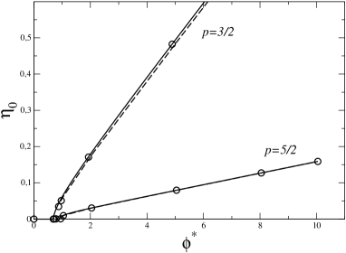
Figure 7: Packing fraction (line coverage) of the condensate as a function of reduced volume fractions $\phi^{*}$, for $p=3/2$ (lower sets) and $p=5/2$ (upper sets). The symbols have been obtained by computing the mean size of the largest particle observed in Monte Carlo simulations, and the curve shows Eq. (118). For the present parameters ($N=1000$), the approximation provided by Eq. (119) proves quite accurate (dashed line, hardly distinguishable from the continuous curve for $p=5/2$).

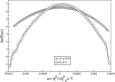
Figure 8: Linear-log plot of the aggregate size distribution for $p=3/2$ and two reduced volume fractions ($\phi^{*}=0.9$ and 2). The data are obtained following over time the different sizes taken by the (unique) condensate. Here, $P$ denotes the probability distribution function of $y=\eta^{p}/\langle\eta_{0}^{p}\rangle-1$.

To confirm the results of section 4 where the condensate volume distribution is calculated, see Eq. (89), we measured the fluctuations in the condensate volume. We find that that the distribution $p(v)$ turns out to be Gaussian, as predicted in section 4 (see Fig. 8). Another prediction is that the fluid phase outside the condensate should have a size distribution of the form (108), irrespective of the reduced volume fraction provided $\phi^{*}>\phi^{*}_{c}$. This expectation is fully consistent with the Monte Carlo results, see Fig. 9 for $p=3/2$. For convenience, we have considered in the main graph the distribution of $\widetilde{\ell}^{p}$, since it is predicted to be a pure exponential. We have performed a similar analysis at $p=5/2$, for various volume fractions beyond the critical one, and the same conclusion holds with again a critical fluid phase, and a size distribution (excluding the condensate) that does not depend on the imposed volume fraction $\phi$. The fluid phase can only accommodate a well defined finite fraction of the total volume (or length), so that when $\phi^{*}$ increases above $\phi^{*}_{c}$, the extra volume is transferred to the aggregate (see Fig. 7).

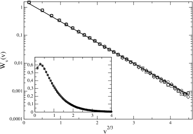
Figure 9: Linear-log plot of the probability distribution function $W_{v}$ of particle “volumes” $v=\widetilde{\ell}^{p}$ as a function of $\widetilde{\ell}$, for $p=3/2$ and several reduced volume fractions beyond the condensation transition (circles for $\phi^{*}=2$, squares for $\phi^{*}=5$ and diamonds for $\phi^{*}=8$). Here $\phi^{*}_{c}=4(2/\pi)^{1/3}/5\simeq 0.688$. The continuous curve shows the prediction of Eq. (108). The inset shows the probability distribution of the variable $\widetilde{\ell}$ instead of $\widetilde{\ell}^{p}$, again as a function of $\widetilde{\ell}=v^{1/p}$.)

VII Conclusion

We have considered a simple stochastic model of mass transport where a real-space condensation takes place upon increasing the volume fraction. The system studied consists of $p$-spheres, constrained to move on a ring, with hard core constraints : the left to left particle distance $x_{i}$ between $p$-spheres $i$ and $i+1$ should exceed the diameter $\ell_{i}$ of $p$-sphere $i$ (see Fig. 1). The latter quantity is itself related to the volume of the sphere through $\ell_{i}=v_{i}^{1/p}$, where $p$ has been retained as a parameter. The total volume of the particles, $\sum_{i}v_{i}$, is fixed, so that the present model involves two conserved quantities ($\sum_{i}x_{i}$, the total length available, and the total volume $V=\sum_{i}v_{i}$). The dynamics comprises diffusion (which can be seen as a stochastic exchange of the quantity $x$ between neighbouring particles), and a stochastic exchange of volume. When $p>1$ and beyond a critical density that has been worked out explicitly, a particle of macroscopically large “mass” (large volume) appears, carrying a finite fraction of the system total volume $V$, surrounded by a critical fluid phase, with a size distribution independent of the total density.

Under mild conditions pertaining to the sampling of the conserved quantities, we have shown that the system admits a factorized steady state probability density, with detailed balance between allowed configurations (essentially those with no overlaps between the $p$-spheres). This allows us to use an alternative description of the system in terms of finding the equilibrium distribution of an ensemble of hard rods, that do not have a quenched size distribution, but can exchange length provided the global constraint $\sum_{i}\ell_{i}^{p}$ remains fixed. Formulated as such, the problem appears as the one dimensional analogue of the optimal polydispersity studies of hard discs and hard sphere fluids ZBTCF99 ; B00 ; BC01 ; CS02 (for instance, the problem studied in ZBTCF99 corresponds to the three dimensional hard sphere situation with $p=1$). The phase transition reported in ZBTCF99 ; B00 ; BC01 ; CS02 can therefore be seen as a condensation arising from constraints in the configuration space.

We have characterized the scenario at work for this transition, and obtained analytically the probability distributions of volumes, gap distance $g$, and left to left particle distance $x$. Restricting to the volume distribution, we have shown that a density functional approach supplemented with scaling considerations allows to recover the results derived from the stochastic processes viewpoint (working out the consequences of the factorization property of the steady state). In this respect, the problem is to find the polydispersity of a hard rod system that will minimize its free energy, given that the total number of rods is fixed as that the $p$ moment of the diameter distribution is fixed as well. The consistent predictions of both approaches have finally been successfully tested against Monte Carlo simulations. It is remarkable that this optimality problem leads to a phase transition in a 1D system, where the condensate size can be considered as an order parameter (note that the constraints imposed introduce a global coupling between all particles). It should also be emphasized that whereas the higher dimensional systems in two or three dimensions could exhibit a transition for $p=1$ (with the convention that the conserved quantity for hard spheres in $d$ dimensions is $\langle\ell^{dp}\rangle$), such a value for $p$-spheres on a line turns out to be critical with however no transition observed: a macroscopic aggregate can only form provided $p>1$.

An important question that remains is that of the dynamic pathways to condensation, that is, how does a single condensate emerge from some given initial condition for the $p$-sphere volumes. As the condensation is driven by constraints in configuration space the dynamics too might be strongly affected by constraints, possibly producing, for example, entropic barriers. This issue remains to be explored.

Acknowledgements : M.R.E. and I. P. thank CNRS and LPTMS, Orsay for hospitality. E.T. acknowledges the hospitality of the Fundamental Physics Department of the University of Barcelona, where part of this work was performed. I.P. acknowledges financial support from MICINN (FIS2008-04386) and DURSI (2005SGR00236). We would also like to thank M.I. García de Soria and P. Maynar for useful discussions.

Appendix A

In this appendix we show that the grand canonical entropy $S(u)$ defined in (41) as

$$S(u)=-(p+1)\,\ln\rho-(p+1)\,\ln F_{\rho}(u)+\ln H(u)+F_{\rho}(u)+u\,F_{\phi}(u).$$ (120)

is maximised when the scaling variable $u$ takes the values zero.

Expanding about $u=0$ to second order in $u=0$ and using the definitions of $H(u)$, $F_{\rho}(u)$ and $F_{\phi}(u)$ given in section 3.2 we obtain

$$S(u)=\left(1+p-(1+p)\ln(1+p)+\ln\left[\Gamma(1+p)\right]\right)+a_{1}u+a_{2}u^{2}+O(u^{3})$$ (121)

where

$$a_{1} = 0$$ (122)

$$a_{2} = [(1+p+p^{2})\Gamma^{2}(2p)-(1+p)\Gamma(p)\Gamma(3p)]/[2(1+p)\Gamma^{2}(p)]$$ (123)

The first equation shows that $u=0$ is a stationary point. The function

$$c(p)=(1+p+p^{2})\Gamma^{2}(2p)-(1+p)\Gamma(p)\Gamma(3p)$$ (124)

is maximised at $p=0.614413$ where its value $c(p)=-0.566304$ is negative. Hence $c(p)$ is negative for all $p>0$, which implies $a_{2}<0$ for all $p>0$ proving indeed that at $u=0$, $S(u)$ is a maximum.

Appendix B

To find out what does determine $\eta_{0}$ (and thus $\eta_{{}_{\cal M}}$) for a given value of $\eta$, we reconsider the free energy functional (90), supplemented with two Lagrange terms to fulfil the constraints ZBTCF99 ; B00 ; BC01

$${\cal R}(W)=\beta{\cal F}(W)\,+\,N{\cal L}_{0}\int W(\ell){\rm d}\ell\,+\,N{\cal L}_{p}\,\left(\int\ell^{p}W(l)\,{\rm d}\ell+L_{0}^{p}\right).$$ (125)

We have to minimize this expression with respect to $W$ and $V_{0}$. Stationarity with respect to $W$ leads to an expression of the form (105):

$$\log[\ell^{1-p}W(\ell)]+\frac{\delta\beta{\cal F}_{\hbox{\scriptsize ex}}}{N\delta W(\ell)}+{\cal L}_{0}+{\cal L}_{p}\ell^{p}=0,$$ (126)

while the derivative with respect to $V_{0}$ reads

$$\frac{\partial{\cal R}}{\partial L_{0}}\,=\,\frac{\partial\beta{\cal F}}{\partial L_{0}}+pN{\cal L}_{p}L_{0}^{p-1}.$$ (127)

The free energy of the system is a function of $L-L_{0}$, since a constituted aggregate does not contribute to $F$ apart from the confinement it induces on the remaining particles which have free energy $F_{{}_{\cal M}}$: $F(N,L_{0},L)=F_{{}_{\cal M}}(N,L-L_{0})$. Hence, Eq. (127) also reads

$$\frac{\partial{\cal R}}{\partial L_{0}}\,=\,P+Np{\cal L}_{p}L_{0}^{p-1}.$$ (128)

From (105) and (126), we have ${\cal L}_{p}\propto(\eta_{c}-\eta_{{}_{\cal M}})$. On the other hand, a physically acceptable mixture $\cal M$, should have a normalizable size distribution, which imposes $\eta_{{}_{\cal M}}\leq\eta_{c}$. Hence, ${\cal L}_{p}\geq 0$ so that the derivative (127) cannot vanish, and is always positive (a situation already encountered in BC01 ). The minimization with respect to $L_{0}$ therefore leads one to choose for $L_{0}$ the minimum possible value compatible with $\eta_{{}_{\cal M}}\leq\eta_{c}$. The optimal value of $L_{0}$ is thus 0 for $\eta<\eta_{c}$, and such that $\eta_{{}_{\cal M}}=\eta_{c}$ whenever $\eta>\eta_{c}$. In other words

$$\eta_{0}=\left\{\begin{array}[]{c l}0&\hbox{ for }\eta<\eta_{c}\\ \displaystyle\frac{\eta-\eta_{c}}{1-\eta_{c}}&\hbox{ for }\eta>\eta_{c}.\end{array}\right.$$ (129)

References

- (1) M. R. Evans and T. Hanney, J. Phys. A 38, R195 (2005)
- (2) S.N. Majumdar, Les Houches (2008) lecture notes, arXiv:0904:4097
- (3) O.J. O’Loan, M.R. Evans and M.E. Cates, Phys. Rev. E 58, 1404 (1998)
- (4) J. Kaupuzs, R. Mahnke, R.J. Harris Phys. Rev. E 72, 056125 (2005)
- (5) D. van der Meer, K. van der Weele, P. Reimann and D. Lohse J. Stat. Mech.: Theor. Exp., P07021 (2007); J. Torok. Physica A 355 374 (2005).
- (6) Y. Kafri, E. Levine, D. Mukamel, G.M. Schütz and J. Török, Phys. Rev. Lett. 89, 035702 (2002).
- (7) A.G. Angel, M.R. Evans, E. Levine and D. Mukamel, Phys. Rev. E 72, 046132 (2005)
- (8) A. G. Angel, T. Hanney, and M. R. Evans, Phys. Rev. E 73, 016105 (2006)
- (9) S.N. Coppersmith, C.-h. Liu, S. Majumdar, O. Narayan, T.A. Witten Phys. Rev. E., 53, 4673 (1996).
- (10) S.N. Majumdar, S. Krishnamurthy and M. Barma, Phys. Rev. Lett. 81, 3691 (1998); J. Stat. Phys. 99, 1 (2000).
- (11) R. Rajesh and S.N. Majumdar, Phys. Rev. E 63, 036114 (2001).
- (12) E. Bertin, J. Phys. A: Math. Gen. 39, 1539 (2006)
- (13) P. Bialas, Z. Burda, and D. Johnston, Nucl. Phys. B 493, 505 (1997).
- (14) M. R. Evans, Braz. J. Phys. 30, 42 (2000).
- (15) S.N. Majumdar, M. R. Evans, and R. K. P. Zia, Phys. Rev. Lett. 94, 180601 (2005)
- (16) M. R. Evans, S.N. Majumdar, and R. K. P. Zia, J. Stat. Phys. 123 357 (2006)
- (17) R. Blaak and J. A. Cuesta, J. Chem. Phys. 115, 963 (2001)
- (18) J. A. Cuesta and R. P. Sear, Europhys. Lett. 55, 451 (2001) ; Phys. Rev. E 65, 031406l (2002)
- (19) J. Zhang, R. Blaak, E. Trizac, J. A. Cuesta, and D. Frenkel, J. Chem. Phys. 110, 5318 (1999)
- (20) M. R. Evans, T. Hanney, J. Phys. A: Math. Gen. 36 (2003) L441-L447
- (21) L. Tonks, Phys. Rev. 50, 955 (1936).
- (22) M. R. Evans, S.N. Majumdar, R. K. P. Zia, J. Phys. A: Math. Gen 37 (2004) L275
- (23) E. Trizac and I. Pagonabarraga, Am. J. Phys. 76, 777 (2008).
- (24) A. Dragulescu and V. Yakovenko, Physica A 299, 213 (2001); Eur. Phys. J. B 17, 723 (2001).
- (25) R. Blaak, J. Chem. Phys. 112, 9041 (2000).
- (26) J.J. Salacuse and G. Stell, J. Chem. Phys. 77, 3714 (1982).
- (27) see e.g R. Evans, in “Fundamentals of Inhomogeneous Fluids”, edited by D. Henderson (Marcel Dekker, New York, 1992).