Uniaxial strain on gapped graphene

Abstract

We study the effect of uniaxial strain on the electronic band structure of gapped graphene. We consider two types of gapped graphene, one which breaks the symmetry between the two triangular sublattices (staggered model), and another which alternates the bonds on the honeycomb lattice (Kekulé model). In the staggered model, the effect of strains below a critical value is only a shift of the band gap location. In the Kekulé model, as strain is increased, band gap location is initially pinned to a corner of the Brillouin zone while its width diminishes, and after gap closure the location of the contact point begins to shift. Analytic and numerical results are obtained for both the tight-binding and Dirac fermion descriptions of gapped graphene.

1 Introduction

Recently, strain engineering of the electronic structure has been explored as an alternative method in the design of graphene-based electronic circuitry [1]. The approach is based on generating local strains to change the hopping amplitudes in an anisotropic way, which in turn leads to the presence of effective gauge fields for the Dirac electrons [2]. A key finding is that for small and moderate uniaxial deformations the gapless Dirac spectrum is robust, and a gap opens only for large deformations above a particular threshold [3, 4, 5]. More precisely, the presence of anisotropy in the tight-binding hoppings on a honeycomb lattice makes the Dirac points approach each other until they merge at a critical asymmetry, at which point a band gap begins to open [6, 7, 8, 9].

For practical purposes, graphene can be considered as a gapless semiconductor. Nevertheless, gaps of various origins have been identified in graphene. Intrinsically, spin-orbit coupling is responsible for a tiny gap, on the order of $10^{-3}$ meV [10, 11, 12, 13], and electron-electron interactions may render graphene an insulator in vacuum [14]. Extrinsically, interaction with substrates and adlayers can induce a band gap in graphene. Epitaxial graphene has a band gap [15] which has been explained as substrate-induced [16]. Other substrates studied include boron-nitride and Cu [17], Ni [18], and several other metals [19]. Band gaps induced by the adsorption of water and ammonia molecules [20], and alkali metals [21] have been studied theoretically. Generally, there are two ways of inducing a gap in monolayer graphene. One way is the mixing of electronic states with different pseudospins in the same valley, and another way is the mixing of states that belong to different valleys. The former can be achieved by sublattice symmetry breaking which leaves the $A$ and $B$ carbon atoms in different environments, while the latter is produced by certain translational symmetry breakings [21].

The purpose of the present work is to study the effect of uniaxial strain on the band structure of gapped graphene [22]. As we show, the effect depends on the origin of the band gap. If it is induced by $AB$ sublattice symmetry breaking, small and moderate strains do not change the width of the gap, but cause its locations in $k$-space to move in a similar way as those of the corresponding Dirac points in the gapless case. On the other hand, if the band gap is induced by translational symmetry breaking that couples the different valley states, a different behavior emerges. With increasing uniaxial strain, the band gap first diminishes and closes in its fixed location and, afterwards, the neutrality point is shifted in reciprocal lattice as in the gapless case.

Our paper is organized as follows. Section 2 contains our analysis of the relevant tight-binding models. Section 3 contains analysis of the corresponding Dirac equations. Section 4 contains numerical results and their discussion, and Section 5 presents our conclusions.

2 Tight-binding model

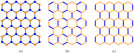
Figure 1: (a) Staggered, (b) Kekulé, and (c) quinoid models.

The models we use can be described as different types of strain distributions [23] shown in Fig. 1. Sublattice symmetry breaking, shown in Fig. 1(a), can be associated with an out-of-plane strain distribution. The so-called Kekulé distortion, shown in Fig. 1(b), breaks the translational symmetry in a way which can be described by a $\sqrt{3}\times\sqrt{3}R30^{\circ}$ commensurate lattice, and can be the result of an in-plane strain distribution. Finally, the quinoid distortion of graphene, shown in Fig. 1(c), represents in-plane uniaxial strain parallel to the nearest-neighbor bond in the vertical direction. Our tight-binding models based on this description are defined by on-site energies and the nearest-neighbor hoppings, but we neglect the change in bond lengths and use the perfect honeycomb lattice.

The primitive unit cell of graphene and the nearest neighbors of the $A$ and $B$ atoms in the unit cell are shown in Fig. 2(a). The tight-binding models involve the vectors $\vec{\delta}$ from an $A$ atom to its nearest-nearest neighbors which are defined in the caption of Fig. 2. The primitive unit cell of the Kekulé model is shown in Fig. 2(b). The Brillouin zone of the Kekulé model and that of graphene, the larger hexagon, are depicted in Fig. 2(c), with special symmetry points defined. In the Kekulé model the points $K$, $K^{\prime}$ and $\Gamma$ belong to the reciprocal lattice and are therefore equivalent, which results in the coupling of the two inequivalent valleys that is responsible for the band gap.

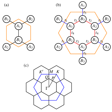
Figure 2: (a) Primitive unit cell of graphene. The vectors $\vec{\delta}$ defined as vectors from atom $A_{1}$ to its nearest neighbors on the $B$ sublattice are given by $\vec{\delta}_{1}=(0,-1/\sqrt{3})a$, $\vec{\delta}_{2}=(1/2,1/2\sqrt{3})a$ and $\vec{\delta}_{3}=(-1/2,1/2\sqrt{3})a$. (b) Kekulé-type graphene primitive unit cell containing its six atom basis. The Kekulé distortion is characterized by two kinds of hoppings, one set around the hexagonal ring (red), and the other set crossing the unit cell boundaries (blue). The addition of a uniaxial strain in the vertical direction results in four hoppings, $t_{1}$, $t_{2}$, $t_{3}$ and $t_{4}$. (c) The relationship between the two Brillouin zones. The path $\Gamma{K}M\Gamma$ is used in the band plots.

A few parameters are needed to define the tight-binding models. In addition to the hopping parameter $t$ ($\approx-2.7$ eV for graphene), there is the band gap of gapped graphene and the asymmetry in hoppings caused by uniaxial strain. We denote by $\Delta$ the half-width of the band gap, and by $\delta{t}$ the shift in one of the hoppings which is in the direction of strain axis. The parameter $t$ may be taken to be positive without loss of generality, and it can serve as the energy scale, so that the models contain two adjustable parameters $\Delta/t$ and $\delta{t}/t$.

The gapped graphene represented by Fig. 1(a) can be described by the tight-binding model with staggered on-site energies $\pm\Delta$. Including the effect of uniaxial strain, we can write the Hamiltonian of this staggered model as

$$H_{s}(\vec{k})=\left(\begin{matrix}-\Delta&h(\vec{k})\\ h^{\ast}(\vec{k})&\Delta\end{matrix}\right),$$ (1)

where

$$h(\vec{k})=(t+\delta{t})e^{i\vec{k}\cdot\vec{\delta}_{1}}+te^{i\vec{k}\cdot\vec{\delta}_{2}}+te^{i\vec{k}\cdot\vec{\delta}_{3}}.$$ (2)

Diagonalizing the Hamiltonian defined by Eq. (1), we find the energy bands,

$$\epsilon_{\pm}(\vec{k})=\pm\sqrt{\Delta^{2}+|h(\vec{k})|^{2}},$$ (3)

which show that the band gap is $\geq 2\Delta$. The function $h(\vec{k})$ is the same as in gapless graphene under strain, where zero modes exist for $\delta{t}/t<1$ and are shifted from $K$ and $K^{\prime}$ toward $M$ [24]. Setting $h(\vec{k})=0$, and taking $k_{y}a=2\pi/\sqrt{3}$ and $k_{x}a=2\pi/3+p_{x}a$, to move along the $KK^{\prime}$ line, we find the shift from $K$ to be

$$p_{x}=\frac{2}{a}\cos^{-1}\left[\frac{1}{2}\left(1+\frac{\delta{t}}{t}\right)\right]-\frac{2\pi}{3a}.$$ (4)

We now turn to the gapped graphene based on Kekulé distortion, shown in Fig. 1(b), which has zero on-site energies but two alternating hoppings, on one-third and two-thirds of the bonds, respectively [21, 25],

$$t_{1}=t+\frac{2}{3}\Delta,\qquad t_{2}=t-\frac{1}{3}\Delta,$$ (5)

where, as in the staggered model, $\Delta$ is half of the energy gap. When uniaxial strain is applied to the Kekulé model, we assume that a shift of $\delta{t}$ is added to the hoppings that are parallel to the strain axis. We define these hoppings as

$$t_{3}=t_{1}+\delta{t},\qquad t_{4}=t_{2}+\delta{t}.$$ (6)

The Hamiltonian of the Kekulé model is given by a $6\times 6$ matrix,

$$H_{K}(\vec{k})=\left(\begin{matrix}\mathbf{0}_{3\times 3}&H_{AB}(\vec{k})\\ H_{BA}(\vec{k})&\mathbf{0}_{3\times 3}\end{matrix}\right),$$ (7)

where the $3\times 3$ block $H_{AB}$ is

$$H_{AB}(\vec{k})=\left(\begin{matrix}t_{2}e^{i\vec{k}\cdot\vec{\delta}_{2}}&t_{2}e^{i\vec{k}\cdot\vec{\delta}_{3}}&t_{3}e^{i\vec{k}\cdot\vec{\delta}_{1}}\\ t_{4}e^{i\vec{k}\cdot\vec{\delta}_{1}}&t_{1}e^{i\vec{k}\cdot\vec{\delta}_{2}}&t_{2}e^{i\vec{k}\cdot\vec{\delta}_{3}}\\ t_{1}e^{i\vec{k}\cdot\vec{\delta}_{3}}&t_{4}e^{i\vec{k}\cdot\vec{\delta}_{1}}&t_{2}e^{i\vec{k}\cdot\vec{\delta}_{2}}\end{matrix}\right),$$ (8)

and $H_{BA}(\vec{k})=H^{\dagger}_{AB}(\vec{k})$. The matrix elements of Eq. (8) have the general form $t_{ij}\exp(i\vec{k}\cdot\vec{\delta}_{ij})$ when linking $A_{i}$ and $B_{j}$ atoms, and can be read off Fig. 2(b).

The band structure of the Kekulé model can be obtained by numerical calculation of the eigenvalues of Eq. (7). However, the existence of zero modes and their locations are determined more simply by

$$\det[H_{K}(\vec{k})]=\left|\det[H_{AB}(\vec{k})]\right|^{2}=0.$$ (9)

Since the zero modes are expected to occur on the horizontal line through $\Gamma$, we calculate the determinant of $H_{AB}$ for $k_{y}=0$,

$$D(k_{x};\Delta/t,\delta{t}/t)=2\,t_{1}\,t_{2}^{2}\cos\frac{3k_{x}a}{2}+t_{3}(t_{4}^{2}-t_{1}^{2})-2\,t_{4}\,t_{2}^{2}.$$ (10)

Setting $D=0$, we find

$$\cos\frac{3k_{x}a}{2}=\frac{2\,t_{4}\,t_{2}^{2}-t_{3}(t_{4}^{2}-t_{1}^{2})}{2\,t_{1}\,t_{2}^{2}},$$ (11)

which has a solution for $k_{x}$ if the right-hand side is in the interval $[-1,1]$. In particular, if $\delta{t}=\Delta$ then $t_{1}=t_{4}$ and the right-hand side of Eq. (11) becomes unity yielding $k_{x}=0$ which is the $\Gamma$ point, or its equivalent $K$ points. Therefore, the gap in the spectrum at $K$ vanishes as $\delta{t}$ is increased from $0$ to $\Delta$. Further increase of $\delta{t}$ then causes the contact points to shift away from the $K$ points, until they merge at $M$, when the right-hand side of Eq. (11) becomes $-1$ and $k_{x}a=2\pi/3$.

3 Dirac equation

We can use the Dirac equation to describe the effect of strain on low-energy electrons provided that both $\Delta/t$ and $\delta{t}/t\ll 1$. The Dirac equation can be derived from the tight-binding model by setting $\vec{k}=\vec{K}+\vec{p}$ near the $K$ and $K^{\prime}$ points. For the staggered model under strain we obtain

$$\mathcal{H}_{s}=\left(\begin{matrix}-\Delta&p^{\ast}+\delta t&0&0\\ p+\delta t&\Delta&0&0\\ 0&0&-\Delta&-p+\delta t\\ 0&0&-p^{\ast}+\delta t&\Delta\end{matrix}\right),$$ (12)

where $p=p_{x}+ip_{y}$ and we have used units such that $\hbar=1$ and $v_{F}=ta\sqrt{3}/2=1$. However, we restore $v_{F}$ explicitly in some of the derived results below. Here we have followed the convention

$$\psi=[\Phi_{KA},\Phi_{KB},\Phi_{K^{\prime}A},\Phi_{K^{\prime}B}]^{T}$$

for the four-dimensional spinor [26]. Our results can be extended to the band gap due to spin-orbit interaction which can be described with a similar Hamiltonian as Eq. (12), except that the gaps have opposite signs for $K$ and $K^{\prime}$ points [10]. The energy dispersions derived from Eq. (12) are given by

$$\epsilon_{\pm}(\vec{p})=\pm\sqrt{(\pm p_{x}+\delta t)^{2}+p_{y}^{2}+\Delta^{2}},$$ (13)

and can be easily verified to be the limiting cases of Eq. (3). The shifts of the Dirac points are $p_{x}=\mp\delta{t}/v_{F}$, which agree with Eq. (4) for $\delta{t}/t\ll 1$.

For the Kekulé model under strain we have

$$\mathcal{H}_{K}=\left(\begin{matrix}0&p^{\ast}+\delta t&0&\Delta\\ p+\delta t&0&\Delta&0\\ 0&\Delta&0&-p+\delta t\\ \Delta&0&-p^{\ast}+\delta t&0\end{matrix}\right),$$ (14)

and the energy eigenvalues are given by

$$\epsilon_{\pm}(\vec{p})=\pm\left[\left(\sqrt{p_{x}^{2}+\Delta^{2}}\pm\delta{t}\right)^{2}+p_{y}^{2}\right]^{1/2}.$$ (15)

For $\delta{t}<\Delta$ there is a gap of size $\Delta-\delta{t}$ at $p=0$. If $\delta{t}\geq\Delta$, zero modes exist at

$$p_{y}=0,\qquad p_{x}=\pm\sqrt{\delta{t}^{2}-\Delta^{2}}.$$ (16)

For $\delta{t}=0$ the energy dispersions, (13) and (15), give identically gapped Dirac spectra, with a density of states (DOS) per unit area given by

$$\rho(\epsilon)=\begin{cases}0,&|\epsilon|<\Delta\\ 2|\epsilon|/\pi{v_{F}^{2}},&\text{otherwise}.\end{cases}$$ (17)

However, for $\delta{t}\neq 0$ the DOS of the staggered model remains the same, while that of the Kekulé model changes as the gap shrinks. For $\delta{t}=\Delta$ and $\epsilon\ll\Delta$, Eq. (15) becomes

$$\epsilon^{2}=\frac{p_{x}^{4}}{4\Delta^{2}}+p_{y}^{2},$$ (18)

which yields a DOS given by

$$\rho(\epsilon)=\frac{2\Gamma(1/4)}{\pi^{3/2}\Gamma(3/4)}\frac{\sqrt{\Delta|\epsilon|}}{v_{F}^{2}}.$$ (19)

4 Numerical results and discussion

Equation (11) can be solved numerically for $k_{x}$ as a function of $\Delta$ and $\delta{t}$. The results for $\Delta=0,t/2,t$ are shown in Fig. 3. For $\Delta=0$ the same curve can be obtained from Eq. (4). For nonzero $\Delta$, the gap first diminishes at $K$ as $\delta{t}$ is increased from $0$ to $\Delta$, and with further increase of $\delta{t}$ the Dirac point moves toward $M$.

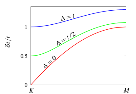
Figure 3: Location of the Dirac point in the Kekulé model along the $KM$ line as a function of $\delta{t}$ for $\Delta=0,t/2,t$. At $M$ the values of $\delta{t}/t$ are $1,\,1.0763,\,1.2996$, respectively.

In Fig. 4 we make plots of Eqs. (13) and (15) for a few values of $\delta{t}$, using $\Delta$ as the scale of energy and momentum. For $\delta{t}=0$, shown in Fig. 4(a), both the staggered and Kekulé models give the same gapped spectrum. However, for $\delta{t}=\Delta$, the valence and conduction bands shift laterally in the $p_{x}$ direction without a change in the gap for the staggered model as in Fig. 4(b). In contrast, for $\delta{t}=\Delta$ the gap closes in the Kekulé model for one pair of bands while the other pair are repelled by $2\Delta$, as in Fig. 4(c). We note that the dispersion is quadratic instead of linear near the degeneracy point as can be expected from Eq. (18). Further increase of $\delta{t}$ to $2\Delta$, shown in Fig. 4(d), causes a shift of the neutrality points in the $p_{x}$ direction, and the dispersions become linear where the bands cross.

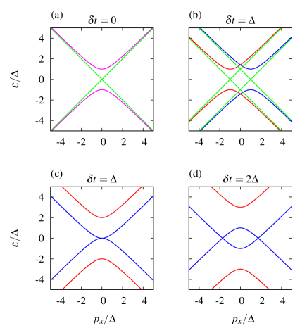
Figure 4: Dirac fermion dispersions along the $p_{y}=0$ line. (a) Gapless and gapped Dirac fermions, with gap equal to $2\Delta$. (b) Strain of $\delta{t}=\Delta$ on gapless and staggered models. (c) Strain of $\delta{t}=\Delta$ on Kekulé model. (d) Strain of $\delta{t}=2\Delta$ on Kekulé model.

Figure 5 shows the band structures from Eq. (3) for $\Delta=0$ and $t/10$. For $\delta{t}=0$, Figs. 5(a) and (b), the Dirac point and the gap, respectively, are located at the $K$ point. For $\delta{t}=t/2$, Figs. 5(c) and (d), they are shifted by the same amount to somewhere along the $KM$ line. For $\delta{t}=t$, Figs. 5(e) and (f), the shift reaches the $M$ point. The last cases are critical in that the Dirac points merge at $M$. We can see that the dispersions are quadratic near $M$ on the $KM$ line, but linear on the $M\Gamma$ line, i.e., a flattening of the Dirac cones takes place which can be seen in contour plots of the band structure (as shown in Ref. 6). For $\delta{t}>1$ a gap opens at the $M$ point for graphene, and the gap of the staggered model becomes wider.

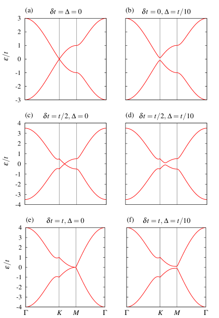
Figure 5: Band structures from the tight-binding model. (a,c,e) show the band structures of graphene for $\delta{t}=0,\,t/2,\,t$, and (b,d,f) show the band structures for the staggered model for the same set of strains.

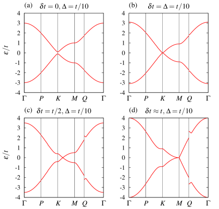
Figure 6: Band structures of the Kekulé tight-binding model for $\delta{t}=0,\,t/10,\,t/2,\,1.00299t$. The extended zone scheme is used.

Figure 6 shows the band structures for the Kekulé model obtained from the numerical evaluation of the eigenvalues of Eq. (7). The band structures are plotted in the extended scheme so they can be compared with those of Fig. 5. The $\Gamma{P}KMQ\Gamma$ path is implied in Fig. 2(c), where $P$ and $Q$ are the points where the path crosses the Brillouin zone of the Kekulé model. It must be remarked that this path does not enclose the irreducible wedge of the Brillouin zone for strained graphene [5, 27], but includes the $KM$ line where the band crossing may occur. Figure 6(a) may be compared with Fig. 5(b) which shows the band structure of the staggered model for the same $\Delta$. The regions of the gap at the $K$ point are similar in both figures, consistent with the Dirac equation description, but there are extra gaps in the band structure of the Kekulé model at $P$ and $Q$. As we have seen in Fig. 4, the gap closes when $\delta{t}=\Delta$ and this can also be seen in Fig. 6(b). Here the dispersion at $K$ is linear on the $PK$ line and quadratic on the $KM$ line. A comparison of Figs. 6(c) and (d) with Fig. 5(c) and (e) shows that in the Kekulé model, after the gap closes, the behavior of the neutrality points are not very different from that in the gapless case.

5 Conclusions

We considered two models of gapped graphene, denoted by staggered and Kekulé, respectively, and studied the effect of strain on their band structures. We found that in the staggered model the width of the band gap does not change for strains less than a critical value, but its locations move following the motion of the Dirac cones in the gapless case. The effect of strain on the band structure of the Kekulé model is less trivial. With increasing strain, reflected in changes in the hoppings, the gap begins to diminish with its locations pinned to the $K$ points. The gap closes when $\delta{t}=\Delta$, i.e., when the shift in hoppings due to strain equals the half-width of the original gap and, afterwards, increasing the strain makes the neutrality point to move in $k$ space as in the gapless case. The effects we have discussed may be observed experimentally in gapped graphene on Ni substrate and epitaxial graphene on SiC, respectively.

6 Acknowledgments

M.F. acknowledges funding from the Iranian Nanotechnology Initiative and H.R.-T. from the Iran National Science Foundation.

References

References

- [1] V. M. Pereira, A. H. Castro Neto, Phys. Rev. Lett. 103 (2009) 046801.
- [2] A. H. Castro Neto, F. Guinea, N. M. R. Peres, K. S. Novoselov, A. K. Geim, Rev. Mod. Phys. 81 (2009) 109.
- [3] V. M. Pereira, A. H. Castro Neto, N. M. R. Peres, Phys. Rev. B 80 (2009) 045401.
- [4] Z. H. Ni, T. Yu, Y. H. Lu, Y. Y. Wang, Y. P. Feng, Z. X. Shen, ACS Nano 3 (2009) 483.
- [5] M. Farjam, H. Rafii-Tabar, Phys. Rev. B 80 (2009) 167401.
- [6] Y. Hasegawa, R. Konno, H. Nakano, M. Kohmoto, Phys. Rev. B 74 (2006) 033413.
- [7] M. O. Goerbig, J.-N. Fuchs, G. Montambaux, F. Piéchon, Phys. Rev. B 78 (2008) 045415.
- [8] G. Montambaux, F. Piéchon, J.-N. Fuchs, M. O. Goerbig, Phys. Rev. B 80 (2009) 153412.
- [9] B. Wunsch, F. Guinea, F. Sols, New J. Phys. 10 (2008) 103027.
- [10] C. L. Kane, E. J. Mele, Phys. Rev. Lett. 95 (2005) 226801.
- [11] H. Min, J. E. Hill, N. A. Sinitsyn, B. R. Sahu, L. Kleinman, A. H. MacDonald, Phys. Rev. B 74 (2006) 165310.
- [12] D. Huertas-Hernando, F. Guinea, A. Brataas, Phys. Rev. B 74 (2006) 155426.
- [13] Y. Yao, F. Ye, X.-L. Qi, S.-C. Zhang, Z. Fang, Phys. Rev. B 75 (2007) 041401(R).
- [14] J. E. Drut, T. A. Lähde, Phys. Rev. Lett. 102 (2009) 026802.
- [15] S. Y. Zhou, G.-H. Gweon, A. V. Fedorov, P. N. First, W. A. de Heer, D.-H. Lee, F. Guinea, A. H. Castro Neto, A. Lanzara, Nat. Mater. 6 (2007) 770.
- [16] S. Kim, J. Ihm, H. J. Choi, Y.-W. Son, Phys. Rev. Lett. 100 (2008) 176802.
- [17] G. Giovannetti, P. A. Khomyakov, G. Brocks, P. J. Kelly, J. van den Brink, Phys. Rev. B 76 (2007) 073103.
- [18] A. Grüneis, D. V. Vyalikh, Phys. Rev. B 77 (2008) 193401.
- [19] P. A. Khomyakov, G. Giovannetti, P. C. Rusu, G. Brocks, J. van den Brink, P. J. Kelly, Phys. Rev. B 79 (2009) 195425.
- [20] R. M. Ribeiro, N. M. R. Peres, J. Coutinho, P. R. Briddon, Phys. Rev. B 78 (2008) 075442.
- [21] M. Farjam, H. Rafii-Tabar, Phys. Rev. B 79 (2009) 045417.
- [22] G. W. Semenoff, V. Semenoff, F. Zhou, Phys. Rev. Lett. 101 (2008) 087204.
- [23] R. Saito, G. Dresselhaus, M. S. Dresselhaus, Physical Properties of Carbon Nanotubes, Imperial College Press, 1998.
- [24] We have limited our discussion to the case of enhancement of the magnitude of hopping. One difference is that when the hopping is reduced the Dirac points move in the opposite direction away from the point, which can be shown by making additional band plots along a different path. However, the main reason to choose enhancement over reduction, is that in the latter the hopping vanishes before the Dirac points can merge and, therefore, this critical region cannot be reached. In real experiments, of course, there are even more severe limitations on how much strain can change the hoppings.
- [25] C.-Y. Hou, C. Chamon, C. Mudry, Phys. Rev. Lett. 98 (2007) 186809.
- [26] J. L. Mañes, F. Guinea, M. A. H. Vozmediano, Phys. Rev. B 75 (2007) 155424.
- [27] G. Gui, J. Li, J. Zhong, Phys. Rev. B 78 (2008) 075435.