Metallicity map of the galaxy cluster A3667

We use XMM-Newton data of the merging cluster Abell 3667 to analyze its metallicity distribution. A detailed abundance map of the central 1.1$\times$1.1 Mpc region indicates that metals are inhomogeneously distributed in the cluster showing a non-uniform and very complex metal pattern. The highest peak in the map corresponds to a cold region, slightly offset South of the X-ray center. This could be interpreted as stripped gas due to a merger between a group moving from NW towards the SE and the main cluster. We note several clumps of high metallicity also in the opposite direction with respect to the X-ray peak. Furthermore we determined abundances for 5 elements (O, Si, S, Ar, Fe) in four different regions of the cluster. Comparisons between these observed abundances and theoretical supernovae yields allow to get constraints on the relative number of SN Ia and II contributing to the enrichment of the intra-cluster medium. To reproduce the observed abundances of the best determined elements (Fe, O and Si) in a region of 7^′ around the X-ray center, 65-80$\%$ of SN II are needed. The comparison between the metal map, a galaxy density map obtained using 550 spectroscopically confirmed cluster members and our simulations suggest a recent merger between the main cluster and the group in the SE.

1 Introduction

Cluster of galaxies are the largest virialized objects in the universe. They form via gravitational instability from the initial perturbations in the matter density field. The cosmic baryons fall into the gravitational potential of the cluster dark matter halo formed in this way, while the collapse heat up the intra-cluster medium (ICM). At the high temperature measured in rich cluster, kT$>$3 keV, the ICM is highly ionised and its spectrum presents several emission lines, among which the most prominent is the Fe K-shell line at $\sim$ 7 keV. As heavy elements are only produced in stars the processed material must have been ejected into the ICM by cluster galaxies.
There is more and more observational evidence that various types of processes are at work (e.g. ram pressure stripping and galactic winds; see Schindler & Diaferio 2008 for a review), which remove interstellar medium (ISM) from the galaxies. Hence, the study of the metal distribution is a sensible way to better understand the thermodynamical properties of the diffuse gas and the past history of star formation in galaxy clusters (Arnaud et al. 1992; Renzini et al. 1993; Renzini 2004).
Simulations have shown that the metal distribution in a cluster shows many stripes and blobs at the positions where the enrichment has taken place. Depending on the dynamical state of the cluster the metal distribution looks very different: in simple merger configuration (e.g. collision between two subclusters) pre-mergers have a metallicity gap between the subclusters, post-mergers have a high metallicity between subclusters (Kapferer et al. 2006; Kapferer et al. 2007; Schindler 2008; Schindler & Diaferio 2008).
Although to obtain metal maps from observation is not easy because a lot of photons have to be accumulated in each region to measure the metal abundance, several groups, using XMM-Newton and Chandra data, have derived quite detailed metallicity maps (Schmidt et al. 2002; Sanders et al. 2004; Durret et al. 2005; O’Sullivan et al. 2005; Sauvageot et al. 2005; Werner et al. 2006; Sanders & Fabian 2006; Hayakawa et al. 2006; Simionescu et al. 2009). In general these 2D maps show that the distribution of metals in cluster is not spherically symmetric, but it has several maxima and complex metal patterns. The range of metallicities measured in a cluster from minimum to maximum comprises easily a factor of two.
Because clusters retain all the metals provided by their galaxies, X-ray measurements of the abundances of each element in the ICM enable us to examine the ratio of SN Ia and II.
In this paper we present the results of the analysis of the cluster Abell 3667 observed with XMM-Newton . The main aim of the work is to study its metal distribution, that can reveal clues about the chemical enrichment history of the cluster (Schindler 2008; Borgani et al. 2008), and to infer its dynamical state by comparison with previous results and hydrodynamic simulations (Kapferer et al. 2006; Kapferer et al. 2007). Secondly, we determine the abundances of several elements and using the yields of Supernovae type Ia and II we try to understand the origin of metals in galaxy clusters.
The paper is structured as follows: in Sect. 2 we give an overview of A3667; in Sect. 3 we present the data sets and data reduction techniques employed and we describe the X-ray image; in Sect. 4 we present the metallicity map and relative comparison with simulations; in Sect 5 we present measurements of metal abundances and SN ratio determination, and in Sect 6 we discuss our results. A summary of our conclusion is given in Sect. 7.
Throughout the paper we assume H₀=70 km s^-1 Mpc^-1, $\Omega_{\Lambda}$=0.73 and $\Omega_{M}$=0.27. At the nominal redshift of A3667 (z=0.055), the luminosity distance is 245.7 Mpc and the angular scale is 64 kpc per arcmin.

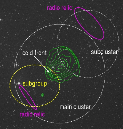
Figure 1: X-ray contours ($green$) overlaid on the optical Digital Sky Survey image. The circles represent the main cluster ($white\ full\ line$) and the northwest subcluster ($dashed\ line$); the ellipses represent the subgroup of 27 members ($dashed\ yellow\ line$) found by Owers et al. (2009) and the two radio relics ($magenta\ lines$). The image is 1${}^{\circ}\times 1^{\circ}$.

2 Abell 3667

A3667, a rich southern cluster at z=0.055 (Sodré et al. 1992), is famous for the presence of two extended radio relics symmetrically located in the cluster periphery in the direction of the elongated X-ray axis (Rottgering et al. 1997). It has a large velocity dispersion (Proust et al. 1988, Sodré et al. 1992, Girardi et al. 1998) and the 2D galaxy distribution is bimodal (Proust et al. 1988, Sodré et al. 1992, Johnston-Hollitt et al. 2008), with the main component around the cD galaxy near the X-ray peak and the secondary component around the second brightest galaxy located in the northwest, $\sim$15^′ from the X-ray center. Owers et al. (2009), with a large number of confirmed galaxy members (550), found evidence for a new subgroup located in the southeast region (see Fig. 1). The bimodal structure is evident also in the weak lensing mass map (Joffre et al. 2000) where it is possible to see a significant mass concentration in the southeast of the cluster but not coincident with the substructure shown by Owers et al. (2009). ROSAT and ASCA observations have shown a distorted X-ray morphology in the direction of the reported bimodal optical distribution (Knopp et al. 1996, Markevitch et al. 1999). XMM-Newton and Chandra observations have revealed an inhomogeneous temperature structure (Mazzotta et al. 2002, Briel et al. 2004) and evidence for a cold front (Vikhlinin et al. 2001). All these features indicate that the cluster suffered a merger recently. Two different scenarios were suggested by Owers et al. (2009). The first is a two-body merger between similar mass structures (the “main cluster” and the NW “subcluster” in Fig. 1) taking place in the plane of the sky. In this scenario the NW subcluster would have already traversed the main cluster along a SE-NW direction, producing two outgoing shocks that would account for the double radio relics observed in A3667. In this case, both the cold front and the subgroup in the southeast of Fig. 1 could have been associated with the northwest cluster, and then sloshed out or tidally stripped during the passage through the core of the main cluster. The SE subgroup could also be a background or foreground structure. An alternative scenario involves a three-body merger between the main cluster and the NW and SE substructures along a NW-SE axis. The NW and SE radio relics would then be associated to the merger between the main cluster and the NW and SE subclusters respectively, and the cold front could be the remnant cold core of the SE subgroup.

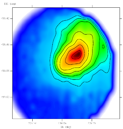
Figure 2: Total (MOS+pn) EPIC mosaic image of A3667 in the [0.5-8] keV. The image is non-background subtracted, corrected for vignetting and exposure and adaptively smoothed. Contours indicate the surface brightness spaced by a factor of $\sqrt{2}$ starting at 5.5$\times$10^-5 cnts s^-1 arcmin^-2 level, which is 3.7 times the average background level. North is up and east is to the left, as they are in all other images. Coordinate grids are shown for the J2000.

3 Observations and data reduction

3.1 X-ray analysis

Observation data files (ODFs) were retrieved from the XMM archive and reprocessed with the XMM-Newton Science Analysis System (SAS) v7.1.0. We used tasks $emchain$ and $epchain$ to generate calibrated event files from raw data. Throughout this analysis single pixel events for the pn data (PATTERN 0) are selected, while for the MOS data sets the PATTERNs 0-12 are used. In addition, for all cameras events next to CCD edges and next to bad pixels were excluded (FLAG==0).
The data were cleaned for periods of high background due to the soft proton solar flares using a two stage filtering process. We first accumulated in 100 s bins the light curve in the [10-12] keV band for MOS and [12-14] keV for pn, where the emission is dominated by the particle-induced background, and exclude all the intervals of exposure time having a count-rate higher than a certain threshold value (the chosen threshold values are 0.20 cps for MOS and 0.25 cps for pn). After filtering using the good time intervals from this screening, the event lists was then re-filtered in a second pass as a safety check for possible flares with soft spectra (Nevalainen et al. 2005; Pradas & Kerp 2005). In this case light curves were made with 10 s bins in the full [0.3-10] keV band. The resulting exposure times after cleaning are 56.6 ks for MOS1, 56.1 ks for MOS2 and 45.7 ks for pn.
To correct for the vignetting effect, we used the photon weighting method (Arnaud et al. 2001). The weight coefficients were computing by applying the SAS task $evigweight$ to each event file. Point sources were detected using the task $ewavelet$ in the energy band [0.3-10] keV and checked by eye on images generated for each detector. We produced a list of selected point sources from all available detectors and the events in the corresponding regions were removed from the event lists.
The background estimates were obtained using the dedicated blank-sky event lists accumulated by Read & Ponman (2003). The blank-sky background events were selected by applying the same PATTERN selection, vignetting correction, flare rejection criteria and point source removal used for the observation events. In addition, we transformed the coordinates of the background file such that they were the same as for the associated cluster data set. The background subtraction was performed using the double subtraction process described in full detail in Arnaud et al. (2002). It involves subtraction of the normalised blank field data, and subsequent subtraction of the cosmic X-ray background component estimated in the area of the field of view that does not show cluster emission.

3.2 X-ray image

As the X-ray morphology can give interesting qualitative (and quantitative, see e.g., Buote & Tsai 1996) insights into the dynamical status of a given cluster, the adaptively smoothed, exposure corrected (MOS+pn) count rate image in the [0.5-8] keV energy band is presented in Fig. 2. The smoothed images was obtained from the raw image corrected for the exposure map by running the task $asmooth$ set to desired signal-to-noise ratio of 20. Regions exposed with less than 10$\%$ of the total exposure were not considered. It is possible to see the elongated structure of the cluster and the cold front to the southeast extensively discussed by Vikhlinin et al. (2001). The distortion in the northwest is introduced by the field of view (FOV) edge. In Fig. 1 we show the X-ray contours superposed on the optical image of the cluster. The X-ray peak lies at RA 20:12.:27 and DEC -56:50:11 (J2000) and is near the central dominant cluster galaxy located at RA 20:12:27 and DEC -56:49:36 (Owers et al. 2007).

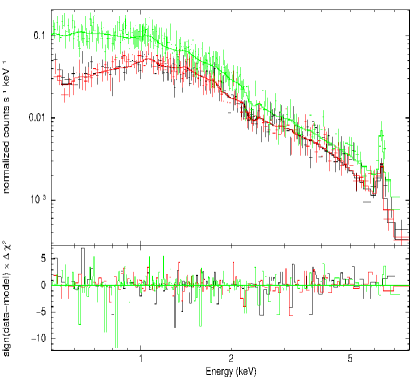
Figure 3: Example of one EPIC pn ($green$) MOS1 ($black$) and MOS2 ($red$) spectrum used to determine the abundance for metallicity map with an error of 10-20$\%$.

4 Metallicity map

To obtain a metallicity measurement with a good accuracy require a high statistic. Based on previous metallicity study we set a minimum count number ($\sim$3,000 source counts per region) necessary for proceeding with the spectral fit. The spectral regions for the map were selected using the following method. We first produced an image where each pixel is 500$\times$500 EPIC physical pixels corresponding to 25${}^{\prime\prime}\times$25^′′. So, from now on “1 pixel” is actually this “fat” 25${}^{\prime\prime}\times$25^′′ “pixel”. A square region with side length of $\sim$1100 arcsec and centred on the peak of the X-ray emission was defined to include only areas where the surface brightness of the source is high. This region was divided into 11$\times$11 square regions, each 100 arcsec². The size of these square regions was then optimized by splitting it into horizontal or vertical segments through its center, while including at least 3,000 source counts, summed over the all three EPIC cameras. Any region which did not contain 3,000 counts was ignored. For all the selected regions, spectra were extracted for source and background in all three cameras. Finally, the spectra were re-binned with the $grppha$ task, to reach at least 20 counts per energy bin.
Spectra were analysed with XSPEC (Arnaud 1996) version 12.3.1. Since the spectra were re-binned, we have used standard $\chi^{2}$ minimization. We determined the errors with the XSPEC tasks $error$ and $steppar$. In order to model the emission from a single temperature we fit the spectra with the following model:

$$MODEL=WABS(N_{H})\times MEKAL(T,Z,K).$$ (1)

WABS is the photoelectric absorption model by Morrison & McCammon (1983) and MeKaL model is the traditional plasma code (Mewe et al. 1985, 1986; Kaastra 1992; Liedahl et al. 1995) in which the temperature T, the metallicity Z and the normalization K are free parameters. The spectral fit was done leaving the hydrogen column density to free vary. We fit jointly MOS1, MOS2 and pn spectra, enforcing the same normalization value for MOS spectra and allowing the pn spectrum to have a separate normalization. In the spectral fitting we used the 0.5-8 and 0.5-7.5 keV energy range for MOS and pn spectra respectively. We excluded the energy above 7.5 keV in the pn spectra because of the strong fluorescence lines of Ni, Cu $\&$ Zn. These lines, present in the background, are not well subtracted by the double background subtraction because they do not scale perfectly with the continuum of the particle-induced background. The redistribution and ancillary files (RMF and ARF) were created with the SAS tasks $rmfgen$ and $arfgen$ for each camera and each region that we analysed. The metal abundances are based on the solar values given by Anders & Grevesse (1989). We chose to use these abundance for easier comparison with previous work, although these values may not be accurate as shown by Grevesse & Sauval (1998) who obtained significantly lower O and Fe abundance then Anders & Grevesse (1989). In Fig. 3 we show an example of the spectra.
The obtained metallicity and temperature maps are shown in Figs. 4 and 6 ($upper\ panel$). The resolution of the maps is the same (although it would be possible to obtain a good estimate of the temperature within smaller region) for a direct comparison between the two maps. Regions in white are those where the spectral signal to noise ratio was not sufficient to determine the metallicity. Both maps show a complex substructure as expected for a merging cluster. In particular the metallicity distribution appears very inhomogeneous, while the temperature map shows a hot arc-like structure around the cold gas region. The highest peak of the metallicity is located in the southeast with respect to the X-ray center corresponding to the cold front region. A higher metallicity is also observed in two blobs to the NW. Between those clumps we note a region with a very low metallicity (below 0.2 in solar abundances).
The histograms in Fig. 4 and 6 ($lower\ panel$) shows the distribution of the metallicity and temperature values. Concerning the metallicity we note that all the values range between 0.05 and 0.7 solar abundances with a mean of $\sim$0.31 Z_⊙ that is in good agreement with the value of 0.29 obtained by fitting the spectra of the whole cluster within a radius of $\sim$8 arcmin centered on the emission peak.
Typical errors in our metallicity map are about 10-20$\%$, although for a few pixels in the outskirts the error is higher. In Fig. 5 we show the 1$\sigma$ upper and lower limits for comparison. For the temperature maps all the errors are lower than 10$\%$.

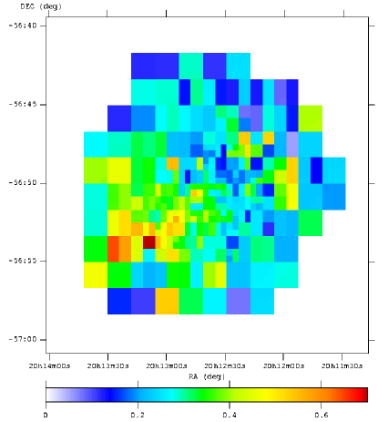
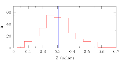
Figure 4: $Upper\ panel$: Metallicity map based on spectra from all three EPIC camera. The scale for the metallicity is in solar units. $Lower\ panel$: Number of bins with a certain metallicity. The vertical line in blue represents the mean value.

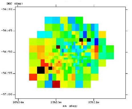
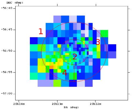
Figure 5: Metallicity map for 1$\sigma$ upper ($top$) and lower ($bottom$) limits, displaced in the same color scale. The numbers indicate the four selected regions used for the abundances determination.

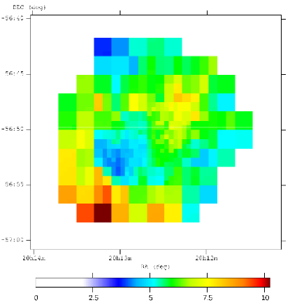
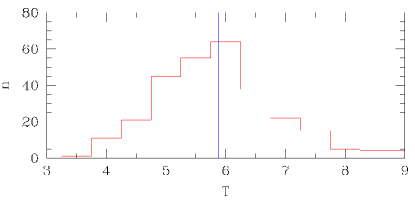
Figure 6: $Upper\ panel$: Temperature map based on spectra from all three EPIC cameras. $Lower\ panel$: Number of bins with a certain temperature. The vertical line in blue represents the mean value.

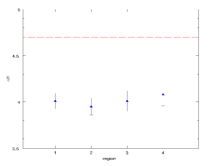
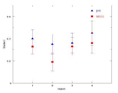
Figure 7: $Upper\ panel$: The hydrogen column density value obtained with a MeKaL model for the 4 considered regions using the all three EPIC cameras (MOS+pn). The red dashed line represent the value obtained by Dickey & Lockman (1990). $Lower\ panel$: Oxygen values obtained by fitting spectra from the MOS and pn detectors independently with the column density fixed to the value computed with a MeKaL model.

5 Abundances and enrichment by supernova type Ia and II

The chemical evolution of galaxies and consequently of the ICM is dominated by its main contributors SN Ia, SN II and planetary nebulae (the contribution of planetary nebulae is negligible for abundances of elements from O to Ni). We investigated the relative contribution of the supernova type Ia/II to the total enrichment on the intra-cluster medium. We assumed that the total number of atoms N_i of the elements $i$ is a linear combination of the number of atoms Y_i produced per supernova type Ia (Y_i,Ia) and type II (Y_i,II):

$$N_{i}=\alpha Y_{i,Ia}+\beta Y_{i,II},$$ (2)

where $\alpha$ and $\beta$ are the numbers of supernova types Ia and II respectively. We used SNIa yields obtained from two different models adapted from Iwamoto et al. (1999): the W7 model is a so-called slow deflagration model, while WDD2 is the favored model by Iwamoto et al. (1999) and is calculated using a delayed detonation model. For nucleosynthesis products of SN II we adopted average yields of stars in a mass range from 10 M_⊙ to 50 M_⊙ calculated by Tsujimoto et al. (1995) assuming a Salpeter initial mass function (IMF).
From observations we obtained the number of nuclei per hydrogen nucleus relative to the solar abundances:

$$\frac{N_{i}}{N_{H}}=f_{i}{\left(\frac{N_{i}}{N_{H}}\right)}_{\odot},$$ (3)

where N_H is the number of hydrogen atoms and $f_{i}$ the abundance obtained directly from XSPEC analysis. Combining equations 2 and 3 and considering iron as fixed element we can compute the ratio between supernova type Ia and II:

$$\frac{\alpha}{\beta}=\frac{{\left(\frac{Fe}{f_{Fe}}-\frac{N_{i}}{f_{i}}\right)}_{SNII}}{{\left(\frac{N_{i}}{f_{i}}-\frac{Fe}{f_{Fe}}\right)}_{SNIa}},$$ (4)

where $Fe$ in the equation is the yield value for the iron. We chose to fix iron because is the best determined element.
We wanted to determine if the high metallicity region is associated with a particular kind of SN type or with high number of SNe II as consequence of an intense episode of star formation, due for instance to ram-pressure effect (Kapferer et al. 2009). To do this we selected four regions: first we extracted the spectra from a circular region, centered on the X-ray peak, with a radius of 3^′ (region 2 in $lower\ panel$ of Fig. 5) ; then we selected an annulus with inner and outer radius of 3^′ and 7^′ respectively and we extracted a spectrum for the low metallicity region by selecting a sector between PA = 180^∘ and 90^∘ (East to West) and for the high metallicity region selecting the sector between PA = 90^∘ and 180^∘ (respectively region 3 and 4); finally, we extracted the spectra from a circle with a radius of 7^′ (region 1) that includes all the three previous regions.

5.1 Abundances determination

In Table 1 we show the obtained abundances with their $\pm$1$\sigma$ errors for one parameter for the four selected regions. We fitted the data with the following procedure to avoid the degeneracy of the parameters: (1) we fitted the data with an absorbed MEKAL model in the 0.4-7 keV band to obtain temperature and nH (metallicity and normalization are considered free parameters); (2) we fixed nH and temperature and use a VMEKAL model in the same energy band to determine the iron abundance (O, Si, S, Ar are left free, the other elements are fixed to the solar value); (3) we kept temperature and iron fixed to measure oxygen abundance in the 0.4-1.5 keV band; (4) we fix the values of temperature, iron and oxygen to estimate the silicon, sulfur and argon abundances in the 1.5-5 keV band.
We fitted the element abundances in narrow bands around to the corresponding emission lines, allowing the normalization to vary, in order to correct for small inaccuracies in the best determination of the continuum in those narrow energy band.
The Ne and Mg abundances could not be constrained because these lines are blended with the Fe-L complex at the EPIC spectral resolution. The aluminium line is blended with the much stronger silicon line and is not measurable. The Ni abundance determinations are driven almost entirely by the He-like and H-like K-shell lines at 7.77 and 8.10 keV which are both beyond the chosen spectral fitting band.
In Fig. 7 ($upper\ panel$) we show the hydrogen column density obtained in all the four analyzed regions. We note that is always lower than the Galactic value of 4.7$\times$10²⁰ cm^-2 determined from the 21 cm radio observation Dickey & Lockman (1990). We left free nH (not fixed to the Galactic value) because of the large discrepancy and also because the O abundance determination is sensitive to the presence of excess absorption and to the cross-calibration uncertainties between the spectral response of the two EPIC instruments in the soft energy band (below 1 keV). In the $lower\ panel$ of Fig. 7 we show the oxygen abundance in the four different regions obtained by fitting the spectra from the MOS and pn detectors separately with N_H fixed at the value obtained with a MEKAL model in the 0.4-7 keV band. The agreement between the two detectors is quite good; the discrepancy in the central 3^′ (region 2) can be due to a calibration problem at this particular position of the detector.

Table 1: Abundances obtained by fitting the four selected regions shown in Fig. 5. Temperatures are given in keV, N_H in 10²⁰ cm^-2 and abundances are given with respect to solar. All errors quoted are at the 68$\%$ level for one interesting parameter ($\Delta{\chi}^{2}$=1).

Par.	1	2	3	4
NH	4.01$\pm$0.08	3.95$\pm$0.09	4.01$\pm$0.11	4.08$\pm$0.12
kT	5.919$\pm$0.035	6.157$\pm$0.053	6.516$\pm$0.068	5.050$\pm$0.049
O	0.34$\pm$0.05	0.26$\pm$0.06	0.30$\pm$0.07	0.40$\pm$0.07
Si	0.43$\pm$0.07	0.37$\pm$0.08	0.35$\pm$0.07	0.52$\pm$0.08
S	0.18$\pm$0.10	0.21$\pm$0.10	0.12$\pm$0.10	0.22$\pm$0.10
Ar	0.28$\pm$0.11	0.27$\pm$0.18	0.24$\pm$0.20	0.36$\pm$0.20
Fe	0.306$\pm$0.009	0.288$\pm$0.010	0.275$\pm$0.014	0.369$\pm$0.013
$\chi^{2}_{Red}$	1.58	1.19	1.23	1.23

Table 2: Relative number of SN II contributing to the enrichment of the intra-cluster medium. We show the results for different region extractions using the yields of SN Ia and SN II, with two physically different SN Ia yield models. In the second column we indicate the element used in combination with iron to determine the percentage number of SN II.

Model	el.	1	2	3	4
W7	O	72.6${}^{+3.7}_{-4.6}$	66.5${}^{+6.1}_{-7.9}$	72.0${}^{+5.8}_{-6.7}$	71.9${}^{+4.4}_{-5.7}$
	Si	75.0${}^{+6.6}_{-9.9}$	70.3${}^{+9.5}_{-16}$	69.8${}^{+8}_{-15}$	75.1${}^{+6.3}_{-9.2}$
	S	$<$55.4	$<$70.4	$<$36.6	$<$48.8
	Ar	83${}^{+12}_{-45}$	84${}^{+15}_{-84}$	81${}^{+19}_{-81}$	86${}^{+23}_{-86}$
WDD2	O	75.5${}^{+3.4}_{-4.2}$	70.0${}^{+5.5}_{-7.4}$	75.0${}^{+5.2}_{-7.1}$	74.9${}^{+3}_{-5.1}$
	Si	74.3${}^{+7.4}_{-11.8}$	69.0${}^{+11}_{-21}$	68.3${}^{+10.4}_{-19}$	74.5${}^{+7.0}_{-11}$
	S	$<$23.8	$<$59.5	-	$<$2.1
	Ar	75${}^{+19}_{-75}$	77${}^{+22}_{-77}$	70${}^{+30}_{-70}$	81${}^{+18}_{-81}$

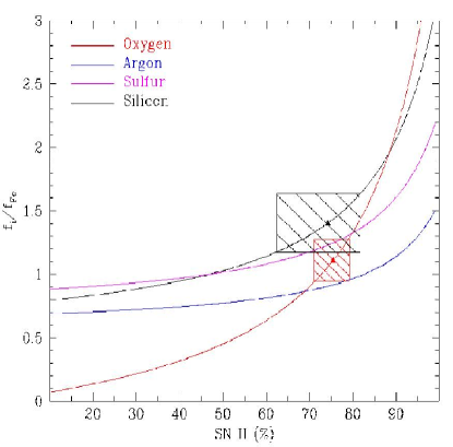
Figure 8: The lines represent the abundance ratios as the SN ratio varying for the different elements. The two solid triangles present the observed O/Fe (red) and Si/Fe (black) ratio for the 7^′ region while the boxes present the error associated with the observed abundance (Y axis) and the relative number of SN II associated with the lower and upper limit (X axis).

6 Discussion

6.1 Metallicity map

There are a number of features to note analyzing the metal map.
First, the metal distribution is very inhomogeneous with several maxima and complex metal patterns as expected for a merging cluster (Kapferer et al. 2006). The X-ray peak is located in a region with a very low metallicity (0.15-0.20 Z_⊙, see Fig. 4) with respect to the mean metallicity of the cluster (0.31 Z_⊙). From the simulations is clear that the maximum of the metallicity is not always in the cluster center (Kapferer et al. 2006). The reason is, that enriched gas, that might fall into the center, is mixed with a lot of other gas as in the centre the gas density is high. Therefore it hardly increases the metallicity there. If, however, a starburst happens in the outer parts of the cluster, the enriched gas mixed only with a small amount of other gas and therefore it can increase the metallicity there considerably. Hence it can happen that the maximum of the metallicity is temporarily not in the cluster centre.
Althouh several blobs with high metallicity ($\sim$0.5 Z_⊙) are present in the NW direction along the axis of the X-ray elongation we found that the most metal rich zone correspond to the cold front region, as previously shown by Briel et al. (2004), with a peak of 0.7 solar abundance. This region probably shows the most interesting feature in the metal map and it can be used together with simulations to infer the dynamical state of the cluster.

6.2 SN enrichment

In Table 2 we show the obtained best fit values of the relative contribution of SN II with a confidence level of 68$\%$. We see that both models are consistent with a scenario where the relative number of supernovae type II contributing to the enrichment of the intra-cluster medium is 55-95$\%$ depending on the considered elements and regions. The best agreement between the data of O, Si, Ar and Fe is obtained using the WDD2 model, although the error bars are quite large due to the uncertainties both in the observations and in the theoretical yields. The relative number of SN II seems to be higher in the metallicity peak region (4), and lower for the regions 2 and 3. The lowest value is obtained in the center (region 2) and it is consistent with the idea of an excess of SN Ia in the cD galaxies (Werner et al. 2008).
The measured abundances of S are quite low and also considering the 1$\sigma$ upper limit the percentage of SN II that we derive is not consistent with the results given by the other elements. We note that the relative low value of 0.18 obtained for the abundances of S in a radius of 7^′ is in good agreement with the value of 0.20 computed by Briel et al. (2004) for the whole cluster. This value agrees also with the result of the sulfur abundance obtained with ASCA data for a sample of clusters with the same temperature as A3667 (Baumgartner et al. 2005) confirming both the prevalence of SN II in the enrichment and a reduced S yield in the SN II model.
We note that for all the elements the lower relative error is larger than the upper one in the relative SN II determination. To explain the reason for it, we combine the equations 2 and 3, and we find

$$\frac{f_{i}}{f_{Fe}}=\frac{N_{i,II}\frac{\alpha}{\beta}+N_{i,I}}{Fe_{II}+Fe_{I}\frac{\alpha}{\beta}},$$ (5)

that gives the theoretical abundance ratio $f_{i}/f_{Fe}$ for varying SN type Ia/II ratios. We show in Fig. 8 the $f_{i}/f_{Fe}$ obtained using the yields of the WDD2 model for supernovae type Ia. It is clear that not all the values of $f_{i}/f_{Fe}$ are allowed: for example the Ar/Fe abundance ratio must be in the range between 0.7 and 1.5. In Fig. 8 we see that all the curves grow very slowly for a low percentage of SN II and they become very steep when that percentage increases. This implies that the determination of the SN fraction becomes quite inaccurate when the relative number of SN II is low, in particular for S/Fe and Ar/Fe that shows a very flat curve when the number of SN II is lower than 60$\%$ of the total supernovae. If we consider symmetric error bars for $f_{i}/f_{Fe}$ it is clear why for the lower relative error in the SN II determination is always larger than the upper one. This does not influence too much the determination of the SN relative number only if the curve is very steep as for example the case of the O/Fe ratio.
To obtain the best agreement between the observed abundances of O, Si, Ar and Fe for the 7^′ region we estimated that 65-80$\%$ of SN II are necessary. Other authors tried to determine the ratio of SN Ia to SN II events in relaxed galaxy clusters by aiming for a best fit to an overall solar abundance pattern from O to Ni. Werner et al. (2006) found that the number contribution of SN II with respect to the total number of supernovae is $\sim$75$\%$, de Plaa et al. (2006) constrained this number to the range 50-75$\%$ while Simionescu et al. (2009) estimated a 30-40$\%$ contribution by SN Ia compared to type II. These results suggest that so far the enrichment of the ICM is mainly due to SN II. We note that Pipino et al. (2002) using different chemical evolution models for galaxies, showed that SN II dominate the chemical enrichment inside the galaxies, while Ia supernovae play a predominant role in the ICM, that is not in agreement with the observational results.
When we interpret the supernovae ratio we have to take into account that the abundances ratio does not only depend on stellar yields and IMF but also on the timescales of production of various elements (Matteucci & Chiappini 2005). The abundance ratios will tend to the ratios of their yield per stellar generation only if the global metal production is considered (metals in stars, gas inside and outside the galaxies), but it fails if only the metals in the individual component are taken into account (e.g. the gas of ICM). Thus, the supernovae estimation listed above should be interpreted as the number of supernovae that would be needed to reproduce the same abundances observed in the ICM, and not the number of supernovae during the history of the cluster.
It is interesting to compare the estimated values with the ones obtained for the galaxies. Leaman (2008) shows the results of the Lick Observatory Supernova Search (LOSS) and in particular he focuses on the determination of the supernovae in the local universe. He found that about 62$\%$ of the SNe observed in galaxies are SN II. In order to reproduce the observed abundances, Tsujimoto et al. (1995) determined the percentage of SN II for our Galaxy to be $\sim$87$\%$, while it is $\sim$77$\%$ and $\sim$83$\%$ for the Large and Small Magellanic Clouds respectively. The relative contribution to the enrichment of ICM by SN II in A3667 is between these values.

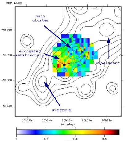
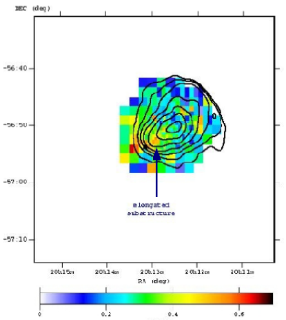
Figure 9: Metallicity maps with the galaxies isodensity ($left$) and X-ray ($right$) contours superimposed. The scale of the metallicity is in solar units. An elongated substructure, both in optical and X-ray contours is shown.

6.3 Comparison to simulations

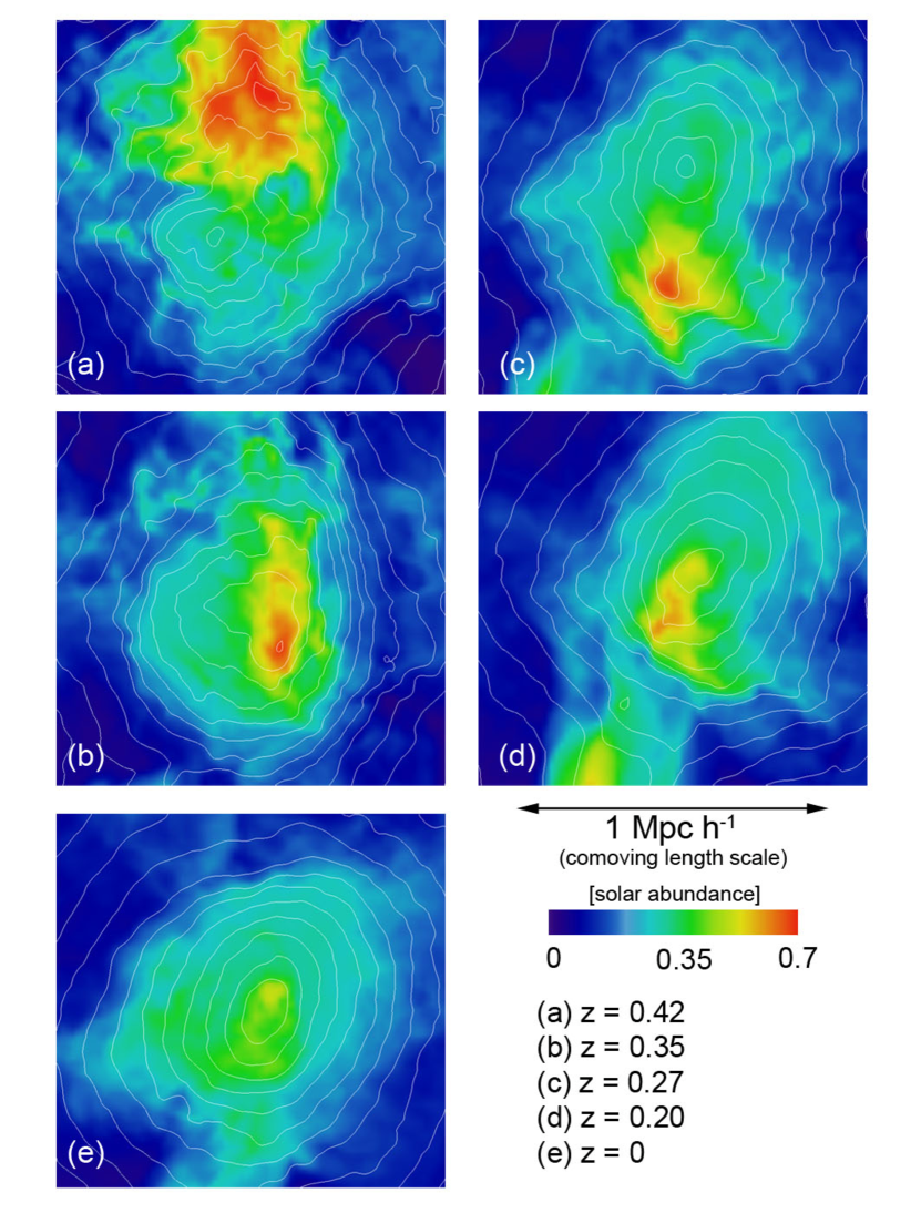
Figure 10: Simulated X-ray weighted metal maps. X-ray surface brightness contours are overlaid. A model cluster showing similar features in the metallicity distribution as A3667 as been selected. The five maps correspond to different redshifts: (a) z=0.42, (b) z=0.35, (c) z=0.27, (d) z=0.2 and (e) z=0.

Simulations of the enrichment of the ICM are a powerful tool to investigate the strengths of different enrichment processes and their spatial and temporal behavior. To study the origin of the inhomogeneities found in the metal distributions in many galaxy clusters, several simulations were performed. In the numerical setup we used different code modules to calculate the main components of a galaxy cluster in the framework of a standard $\Lambda$CDM cosmology. The non-baryonic dark matter (DM) component is calculated using GADGET2 (Springel 2005) with constrained random field initial conditions (Hoffman & Ribak 1991), implemented by van de Weygaert & Bertschinger (1996). For the treatment of the ICM we use comoving Eulerian hydrodynamic with a shock capturing schemes (PPM, Colella & Woodward 1984), with a fixed mesh refinement (Ruffert 1992) on four levels and radiative cooling (Sutherland & Dopita 1993). The properties of the galaxies are calculated by an improved version (van Kampen et al. 2005) of the galaxy formation code of van Kampen et al. (1999) which is a semi-analytic model in the sense that the merging history of galaxy halo is taken directly from the cosmological N-body simulation. With this setup we investigated two different enrichment processes, namely supernova driven galactic winds and ram-pressure stripping (see Kapferer et al. 2009 for details regarding the galactic winds model and Domainko et al. 2006 for the ram-pressure stripping model).
In Fig. 10 the evolution of the metallicity in a model cluster is shown. The isolines correspond to the X-ray surface brightness of the model cluster. In the simulation a region of enriched material falls towards the cluster center. The high metallicity is in this infall region (see at the top of panel (a) in Fig. 10) and it is caused by four starbursts (with an outflow rate of more than 25 solar masses each) that happened before z=0.42. Approaching the cluster center the material gets mixed with the lower metallicity ICM along the trajectory (see panel (b) in Fig. 10). From the turnaround point (see panel (c) Fig. 10) the material falls smoothly to the center and gets mixed by the ambient ICM with lower metallicity (see panel (d) Fig. 10). As the material ejected by galactic winds and starbursts contains more SNII products the feature in the simulation (panel (d) in Fig. 10) corresponds nicely to the off-center metal concentration found in A3667 (see Fig. 4) where the relative contribution of the SN II is higher (region 4). At a redshift of z=0 the enriched gas originating from starbursts has already mixed with the ICM, leading to the metal map shown in panel (d) in Fig. 10.
Metal blobs originating either from galactic winds or ram-pressure stripping are a common feature in metal enrichment simulations. Typically they move along the trajectory of the underlying galaxies and as they start to feel the pressure of the surrounding gas they lag behind the originating galaxies and mix with the surrounding gas. The more inhomogeneities are present in the ICM the more recent the enrichment processes took place. Therefore the inhomogeneities found in the metal maps in galaxy clusters are indicators for the merging frequency of substructures with the cluster. Typically the inhomogeneities in the metal maps vanish over timescales of several 100 Myrs to several Gyrs depending to the mass present in the metal feature. In the example in Fig. 10 the metallicity blob survives nearly 3 Gyrs.
Based on the size of the high metallicity region ($\sim$3^′ of radius), we expect that the metal feature in Fig. 4 is either a consequence of a recent merger or of an older merger but which involve a larger mass. In the latter case the metal feature would have survived for a long time.

6.4 Dynamical state

We produced a multi-scale galaxy density map (see Ferrari et al. 2005 for more details) using the 550 spectroscopically confirmed cluster members obtained by Owers et al. (2009). In Fig. 9 we plotted for comparison the metal map with the galaxy isodensity overlaid ($left$) and X-ray ($right$) contours. As for the X-ray surface brightness the projected galaxy density map shows an elongation in the direction of the two radio relics. The comparison of the ICM metallicity distribution and the position of the sub clusters of A3667 can give hints on the complex merging scenario of this cluster (Kapferer et al. 2006). We detected a metal peak between the main cluster and the SE subgroup. According to Kapferer et al. (2006) we expect high metallicity between subclusters in a post-merger phase. Thus, this configuration supports the scenario suggested by Owers et al. (2009) in which the SE subgroup has traveled from the NW and passed through the main cluster where the ram pressure stripped off the enriched and cooler gas.
However, an elongation towards the high metallicity peak visible both in optical and X-ray images (see the contours in Fig. 9) could suggest a more complex dynamics in the cluster center. The abundances of the measured elements are higher in region 4 with respect to the regions 2 and 3. This result can be explained if a group of galaxies, located in the elongated substructure and containing both SN Ia and SN II products, falls into a cluster moving from southeast to northwest. The inter-stellar medium is thus stripped off by ram-pressure stripping and leads to a more peaked abundance distribution. On the other hand, in region 4 the relative number of SN II seems to be higher, with respect to the other two considered regions (region 2 and 3), suggesting that the metallicity peak in region 4 is mainly due to galactic winds as obtained in the simulations. Due to the large error bars in the SN determination the latter result has to be confirmed with a deeper observation.
Interestingly a gap in metallicity has been detected by Briel et al. 2004 in between the main cluster and the NW sub-cluster (i.e. a region not covered by our metallicity map). Based on the results of (Kapferer et al. 2006) this would imply that these two structures are in a pre-merger phase. All these results could suggest that A3667 is a cluster forming through multiple merging events along a common NW-SE axis.

7 Summary

We analyzed a 64 ks XMM-Newton exposure of the merging cluster of galaxies A3667. We obtained a detailed 2D metallicity map. From this we can conclude that:

• the distribution of metals is clearly non-spherical. It looks very inhomogeneous with several maxima separated by very low metallicity regions;

• the highest metallicity peak is located on the southeast with respect to the X-ray center and it corresponds to the region with the lowest temperature.

We also measured the abundances for oxygen, silicon, sulfur, argon and iron in 4 different regions of the cluster and determined the number ratio of supernovae type Ia and type II. From these data we conclude that:

• using the elements abundance of Fe, O and Si we found that the relative number of supernovae type II necessary to reproduce the observed abundances in A3667 ranges between 65-80$\%$;

• the delayed detonation model WDD2 seems to reproduce the observed data better compared to the slow deflagration model;

• the supernovae number estimation from the abundances of sulfur is not in agreement with the estimate obtained using the other elements confirming a reduced S yield in the SN II model.

Finally, we discussed the dynamical state of the cluster by comparing the ICM metal and galaxy density maps to our simulations. In agreement with the scenario proposed by Owers et al. (2009), we conclude that the SE subgroup moved from the NW and passed through the main cluster, where the ram pressure stripped off the enriched and cooler gas as seen in the metallicity and temperature maps. The highest metallicity region, that shows a higher contribution of SN II, could be partly related to an enrichment by galactig winds due to star formation possibly triggered by an infalling group. In addition, two metal rich blobs in the NW of the main cluster could partly result from inhomogeneities not completed dispersed after an old merger, which is possibly responsible for the formation of the two radio relics. Based on the comparison with previous X-ray data (e.g. Briel et al. 2004) we conclude that A3667 has a complex dynamical history and it is possibly evolving by accreting sub-clusters along a main NW-SE axis.

Acknowledgements. We warmly thank Matt Owers for providing the catalog with positions of confirmed cluster members and Jean-Patrick Henry the referee for very useful comments. The authors acknowledge the Austrian Science Foundation (FWF) through grants P18523-N16 and P19300-N16.

References

- Anders & Grevesse (1989) Anders, E. & Grevesse, N. 1989, Geochim. Cosmochim. Acta., 53, 197
- Arnaud (1996) Arnaud, K. A. 1996, in Astronomical Society of the Pacific Conference Series, Vol. 101, Astronomical Data Analysis Software and Systems V, ed. G. H. Jacoby & J. Barnes
- Arnaud et al. (2002) Arnaud, M., Majerowicz, S., Lumb, D., et al. 2002, A&A, 390, 27
- Arnaud et al. (2001) Arnaud, M., Neumann, D. M., Aghanim, N., et al. 2001, A&A, 365, L80
- Arnaud et al. (1992) Arnaud, M., Rothenflug, R., Boulade, O., Vigroux, L., & Vangioni-Flam, E. 1992, A&A, 254, 49
- Baumgartner et al. (2005) Baumgartner, W. H., Loewenstein, M., Horner, D. J., & Mushotzky, R. F. 2005, ApJ, 620, 680
- Borgani et al. (2008) Borgani, S., Fabjan, D., Tornatore, L., et al. 2008, Space Science Reviews, 134, 379
- Briel et al. (2004) Briel, U. G., Finoguenov, A., & Henry, J. P. 2004, A&A, 426, 1
- Buote & Tsai (1996) Buote, D. A. & Tsai, J. C. 1996, ApJ, 458, 27
- Colella & Woodward (1984) Colella, P. & Woodward, P. R. 1984, Journal of Computational Physics, 54, 174
- de Plaa et al. (2006) de Plaa, J., Werner, N., Bykov, A. M., et al. 2006, A&A, 452, 397
- Dickey & Lockman (1990) Dickey, J. M. & Lockman, F. J. 1990, ARA&A, 28, 215
- Domainko et al. (2006) Domainko, W., Mair, M., Kapferer, W., et al. 2006, A&A, 452, 795
- Durret et al. (2005) Durret, F., Lima Neto, G. B., & Forman, W. 2005, A&A, 432, 809
- Ferrari et al. (2005) Ferrari, C., Benoist, C., Maurogordato, S., Cappi, A., & Slezak, E. 2005, A&A, 430, 19
- Girardi et al. (1998) Girardi, M., Giuricin, G., Mardirossian, F., Mezzetti, M., & Boschin, W. 1998, ApJ, 505, 74
- Grevesse & Sauval (1998) Grevesse, N. & Sauval, A. J. 1998, Space Science Reviews, 85, 161
- Hayakawa et al. (2006) Hayakawa, A., Hoshino, A., Ishida, M., et al. 2006, PASJ, 58, 695
- Hoffman & Ribak (1991) Hoffman, Y. & Ribak, E. 1991, ApJ, 380, L5
- Iwamoto et al. (1999) Iwamoto, K., Brachwitz, F., Nomoto, K., et al. 1999, ApJS, 125, 439
- Joffre et al. (2000) Joffre, M., Fischer, P., Frieman, J., et al. 2000, ApJ, 534, L131
- Johnston-Hollitt et al. (2008) Johnston-Hollitt, M., Hunstead, R. W., & Corbett, E. 2008, A&A, 479, 1
- Kaastra (1992) Kaastra, J. S. 1992, An X-ray spectral Code for Optically Thin Plasmas, Internal SRON-Leiden Report,updated version 2.0
- Kapferer (et al. 2009) Kapferer, W. et al. 2009, AA submitted
- Kapferer et al. (2006) Kapferer, W., Ferrari, C., Domainko, W., et al. 2006, A&A, 447, 827
- Kapferer et al. (2007) Kapferer, W., Kronberger, T., Weratschnig, J., et al. 2007, A&A, 466, 813
- Kapferer et al. (2009) Kapferer, W., Sluka, C., Schindler, S., Ferrari, C., & Ziegler, B. 2009, A&A, 499, 87
- Knopp et al. (1996) Knopp, G. P., Henry, J. P., & Briel, U. G. 1996, ApJ, 472, 125
- Leaman (2008) Leaman, J. F. 2008, PhD thesis, University of California, Berkeley
- Liedahl et al. (1995) Liedahl, D. A., Osterheld, A. L., & Goldstein, W. H. 1995, ApJ, 438, L115
- Markevitch et al. (1999) Markevitch, M., Sarazin, C. L., & Vikhlinin, A. 1999, ApJ, 521, 526
- Matteucci & Chiappini (2005) Matteucci, F. & Chiappini, C. 2005, Publications of the Astronomical Society of Australia, 22, 49
- Mazzotta et al. (2002) Mazzotta, P., Fusco-Femiano, R., & Vikhlinin, A. 2002, ApJ, 569, L31
- Mewe et al. (1985) Mewe, R., Gronenschild, E. H. B. M., & van den Oord, G. H. J. 1985, A&AS, 62, 197
- Mewe et al. (1986) Mewe, R., Lemen, J. R., & van den Oord, G. H. J. 1986, A&AS, 65, 511
- Morrison & McCammon (1983) Morrison, R. & McCammon, D. 1983, ApJ, 270, 119
- Nevalainen et al. (2005) Nevalainen, J., Markevitch, M., & Lumb, D. 2005, ApJ, 629, 172
- O’Sullivan et al. (2005) O’Sullivan, E., Vrtilek, J. M., Kempner, J. C., David, L. P., & Houck, J. C. 2005, MNRAS, 357, 1134
- Owers et al. (2007) Owers, M. S., Blake, C., Couch, W. J., Pracy, M. B., & Bekki, K. 2007, MNRAS, 381, 494
- Owers et al. (2009) Owers, M. S., Couch, W. J., & Nulsen, P. E. J. 2009, ApJ, 693, 901
- Pipino et al. (2002) Pipino, A., Matteucci, F., Borgani, S., & Biviano, A. 2002, New Astronomy, 7, 227
- Pradas & Kerp (2005) Pradas, J. & Kerp, J. 2005, A&A, 443, 721
- Proust et al. (1988) Proust, D., Mazure, A., Sodre, L., Capelato, H., & Lund, G. 1988, A&AS, 72, 415
- Read & Ponman (2003) Read, A. M. & Ponman, T. J. 2003, A&A, 409, 395
- Renzini (2004) Renzini, A. 2004, in Clusters of Galaxies: Probes of Cosmological Structure and Galaxy Evolution, ed. J. S. Mulchaey, A. Dressler, & A. Oemler
- Renzini et al. (1993) Renzini, A., Ciotti, L., D’Ercole, A., & Pellegrini, S. 1993, ApJ, 419, 52
- Rottgering et al. (1997) Rottgering, H. J. A., Wieringa, M. H., Hunstead, R. W., & Ekers, R. D. 1997, MNRAS, 290, 577
- Ruffert (1992) Ruffert, M. 1992, A&A, 265, 82
- Sanders & Fabian (2006) Sanders, J. S. & Fabian, A. C. 2006, MNRAS, 371, 1483
- Sanders et al. (2004) Sanders, J. S., Fabian, A. C., Allen, S. W., & Schmidt, R. W. 2004, MNRAS, 349, 952
- Sauvageot et al. (2005) Sauvageot, J. L., Belsole, E., & Pratt, G. W. 2005, A&A, 444, 673
- Schindler (2008) Schindler, S. 2008, Chinese Journal of Astronomy and Astrophysics Supplement, 8, 93
- Schindler & Diaferio (2008) Schindler, S. & Diaferio, A. 2008, Space Science Reviews, 134, 363
- Schmidt et al. (2002) Schmidt, R. W., Fabian, A. C., & Sanders, J. S. 2002, MNRAS, 337, 71
- Simionescu et al. (2009) Simionescu, A., Werner, N., Böhringer, H., et al. 2009, A&A, 493, 409
- Sodré et al. (1992) Sodré, L. J., Capelato, H. V., Steiner, J. E., Proust, D., & Mazure, A. 1992, MNRAS, 259, 233
- Springel (2005) Springel, V. 2005, MNRAS, 364, 1105
- Sutherland & Dopita (1993) Sutherland, R. S. & Dopita, M. A. 1993, ApJS, 88, 253
- Tsujimoto et al. (1995) Tsujimoto, T., Nomoto, K., Yoshii, Y., et al. 1995, MNRAS, 277, 945
- van de Weygaert & Bertschinger (1996) van de Weygaert, R. & Bertschinger, E. 1996, MNRAS, 281, 84
- van Kampen et al. (1999) van Kampen, E., Jimenez, R., & Peacock, J. A. 1999, MNRAS, 310, 43
- van Kampen et al. (2005) van Kampen, E., Percival, W. J., Crawford, M., et al. 2005, MNRAS, 359, 469
- Vikhlinin et al. (2001) Vikhlinin, A., Markevitch, M., & Murray, S. S. 2001, ApJ, 551, 160
- Werner et al. (2006) Werner, N., de Plaa, J., Kaastra, J. S., et al. 2006, A&A, 449, 475
- Werner et al. (2008) Werner, N., Durret, F., Ohashi, T., Schindler, S., & Wiersma, R. P. C. 2008, Space Science Reviews, 134, 337