Evidence for early disk-locking among low-mass members of the Orion Nebula Cluster

Abstract

Context. We present new high-resolution spectroscopic observations for 91 pre-main sequence stars in the Orion Nebular Cluster (ONC) with masses in the range $0.10-0.25M_{\odot}$ carried out with the multi-fiber spectrograph flames attached to the UT2 at the Paranal Observatory.

Aims. Our aim is to better understand the disk-locking scenario in very low-mass stars.

Methods. We have derived radial velocities, projected rotational velocities, and full width at 10% of the H$\alpha$ emission peak. Using published measurements of infrared excess ($\Delta(I_{\rm C}-K)$), as disk tracer and equivalent width of the nead-infrared Ca ii line $\lambda$8542, mid-infrared difference [3.6]$-$[8.0] $\mu$m derived by Spitzer data, and 10% H$\alpha$ width as diagnostic of the level of accretion, we have looked for any correlation between projected angular rotational velocity divided by the radius ($v\sin i/R$) and presence of disk and accretion.

Results. For 4 low-mass stars, the cross-correlation function is clearly double-lined indicating that the stars are SB2 systems. The distribution of rotation periods derived from our $v\sin i$ measurements is unimodal with a peak of few days, in agreement with previous results for $M<0.25M_{\odot}$. The photometric periods were combined with our $v\sin i$ to derive the equatorial velocity and the distribution of rotational axes. Our $<\sin i>$ is lower than the one expected for a random distribution, as previously found. We find no evidence for a population of fast rotators close to the break-up velocity. A clear correlation between $v\sin i/R$ and $\Delta(I_{\rm C}-K)$ has been found. While for stars with no circumstellar disk ($\Delta(I_{\rm C}-K)<0.3$) a spread in the rotation rates is seen, stars with a circumstellar disk ($\Delta(I_{\rm C}-K)>0.3$) show an abrupt drop in their rotation rates by a factor of $\sim 5$. On the other hand, only a partial correlation between $v\sin i$ and accretion is observed when other indicators are used. The X-ray coronal activity level ($\log L_{\rm X}/L_{\rm bol}$) shows no dependence on $v\sin i/R$ suggesting that all stars are in a saturated regime limit. The critical velocity is probably below our $v\sin i$ detection limit of 9 km s^-1.

Conclusions. The ONC low-mass stars in our sample, close to the hydrogen burning limit, at present seem to be not locked, but the clear correlation we find between rotation and infrared color excess suggests that they were locked once. In addition, the percentage of accretors seems to scale inversely to the stellar mass.

1 Introduction

Surface rotation is a key observational parameter for stellar evolution because it is linked to the internal angular momentum transport and to the mechanisms responsible for stellar angular momentum loss. Its initial conditions are set during the star formation process.

There are four main ingredients describing the angular momentum (AM) evolution of $1M_{\odot}$ star: i) Solid body rotation. Stars begin their lives as fully convective objects. Since the timescale for convective transport is much shorter than that for angular momentum loss, the stars probably rotate as solid bodies (Stassun & Tendrup 2003, and references therein). ii) Disk-locking. The idea of magnetic disk-locking originated with the theory developed by Ghosh & Lamb (1979) for neutron stars, but in the context of pre-main sequence (PMS) stars was proposed for the first time by Camenzind (1990) and König (1991). The stellar magnetic field threads the slowly rotating circumstellar disk of the young star, truncating it at several stellar radii (Bouvier et al. 2007). Due to the difference in angular velocity, magnetic torques will transfer angular momentum from the star to the disk causing them to corotate, i.e. the spin-up torque on the star is exactly balanced by a spin-down torque transmitted by the field lines threading the disk beyond the corotation radius. In the end, the stellar rotational angular velocity equals the Keplerian angular velocity of the inner disk (Shu et al. 1994). iii) Stellar winds. Angular momentum loss continues via a magnetized wind during the evolution to and on the main-sequence. The rate of angular momentum loss depends on whether the angular rotation rate is above the saturation limit (Barnes & Sofia 1996). iv) Core-envelope decoupling. Surface rotation is eventually replenished by AM brought from the rapid rotating core in a characteristic time $\tau_{c}$. How the decoupling characteristic depends on mass (and on other stellar parameters) is still unsettled.

Although many details remain to be understood, these four ingredients seem to regulate the broad aspects of the AM evolution from PMS to solar age for $\sim 1M_{\odot}$ stars. Among these four ingredients, the disk-locking hypothesis is believed to play a fundamental role in the early AM evolution during the T-Tauri phase, when young stars are expected to have circumstellar disks. This scenario has been supported through the years by different observational photometric studies which show that T-Tauri stars with disks (CTTS) have significantly longer periods than their disk-less counterparts (WTTS), i.e. they rotate at a small fraction (10–20%) of the break-up velocity (Attridge & Herbst 1992; Bouvier et al. 1993; Edwards et al. 1993; Choi & Herbst 1996; Marilli et al. 2007). This indicates an efficient method for shedding AM, which is contrary to the expectation that these stars should spin close to break-up speed, having recently contracted from their natal clouds (Stassun et al. 1999).

In contrast to the $1M_{\odot}$ mass regime, the AM evolution for lower mass stars is far from being understood. In particular, there are contrasting opinions regarding the distribution of rotational period ($P_{\rm rot}$) for very low-mass stars ($M\la 0.25M_{\odot}$). From an observative point of view, Stassun et al. (1999) have challenged the disk-locking scenario in 254 stars of the young Orion OBIc/d association by showing that there is no evidence for the bimodal period distribution originally attributed to disk braking. In addition, no correlation between observed $P_{\rm rot}$ and accretion diagnostics and no differences between $P_{\rm rot}$ distributions of WTTS and CTTS were found, calling the standard disk-locking scenario into question. Herbst et al. (2000, 2001, 2002) obtain a bimodal period distribution for the Orion Nebula Cluster (ONC) confirming the findings of Choi & Herbst (1996) and point out the dependence of the rotation on mass. They find a bimodal distribution of rotation periods for higher masses ($M\ga 0.25M_{\odot}$) with a gap near 4 days, while lower masses ($M\la 0.25M_{\odot}$) have a unimodal distribution and generally spin faster. They show a statistically significant anti-correlation between IR excess emission and rotation: slower rotators are more likely to show evidence of circumstellar disks. Rebull (2001) looked for the mass dependence in ONC flaking fields, but found only weak evidence for a change in rotational period distribution for low-mass stars. Later, Rebull et al. (2002) have shown that in stars of the ONC and NGC2264 AM is depleted very early during the T-Tauri phase and have concluded that disk-locking is indeed the most likely mechanism to be acting. Hartmann (2002), adopting accretion rates of $\dot{M}\sim 10^{-8.6}M_{\odot}$ yr^-1 taken from Rebull et al. (2000) for the ONC flaking fields for $M\sim 0.3M_{\odot}$ and an initial rotation rate at 10% of the break-up velocity, concluded that the time-scale needed to remove stellar angular momentum by disk-locking is of the order of the ONC age ($\sim 1-3$ Myr). In addition, he suggested that if these properties change with mass in a way to enhance the braking for higher masses, this could explain the bimodal distribution found in some studies. Then, Makidon et al. (2004) report for stars of NGC 2264 ($\sim 2-4$ Myr) no conclusive evidence that more slowly rotating stars show disk indicators or that faster rotating stars are less likely to show disk indicators. Later, Littlefair et al. (2005) find in IC 348 ($\sim 2-4$ Myr) $P_{\rm rot}$ bimodality at $M\ga 0.25M_{\odot}$ and unimodality at $M\la 0.25M_{\odot}$ and claim a strong mass effect as explanation. The same year, Lamm et al. (2005) find evidences of disk-locking for stars of the same OB association, less pronounced for low masses ($M\la 0.25M_{\odot}$). For this mass regime they speak about “moderate angular momentum loss”. More recently, Rebull et al. (2006) and Cieza & Baliber (2007) find that in Orion and NGC 2264 stars with long periods are more likely than those with short periods to have IR excesses suggestive of disks. Very recently, Nguyen et al. (2009) find in Taurus-Auriga and Chamaeleon I ($\sim 2$ Myr) that both accretors and non-accretors have similar distributions of $v\sin i$, while Rodriguez-Ledesma et al. (2009) confirm the result found by Herbst et al. (2000, 2001, 2002) in ONC.

From a theoretical point of view, Matt & Pudritz (2004) critically examined the disk-locking theory and showed that in stars, such as CTTSs, where the magnetic field is strong, it is also highly twisted and disordered. The differential rotation between the star and disk naturally leads to an opening (i.e. disconnecting) of the magnetic field between the two. Consequently, the resulting spin-down torque on the star by the disk is significantly reduced, and the disk-locking model cannot account for accreting stars that spin slowly (e.g., about 10% of the break-up velocity). Hence, the disk-locking scenario does not explain the angular momentum loss of the slow rotators. They conclude that, in order for accreting protostars to spin as slowly as 10% of the break-up speed, there must be spin-down torques acting on the star other than those carried by magnetic field lines connecting the star to the disk. The presence of open stellar field lines leads them to the possibility that excess angular momentum is carried by a stellar wind along those open lines (Matt & Pudritz 2004).

Therefore, it is clear that the angular momentum evolution for very low-mass stars is still not well understood. For a review concerning the rotation and angular momentum evolution of young and very low-mass stars from observative and theoretical points of view, see Herbst & Mundt (2005), Herbst et al. (2007), and Irwin & Bouvier (2009).

In this work we measure H$\alpha$ excesses, projected rotational velocities ($v\sin i$), and radial velocities ($V_{\rm rad}$) of stars in the ONC with masses between 0.10 and 0.25 $M_{\odot}$. The ONC is the nearest large region of on-going star formation. Our study of this star-forming region is aimed at investigating whether there is any observational evidence supporting disk-locking in this still poorly studied mass range. More specifically, in order to shed more light on the disk-locking scenario for very low-mass stars, we look for any relation between rotation and accretion, and rotation and disk presence. We also look for the fast rotators population first reported by Stassun et al. (1999) and compare our rotational velocity distribution to the one derived by Herbst et al. (2000, 2001, 2002).

2 Observations, Data Reduction, and Analysis

2.1 Sample selection and Observations

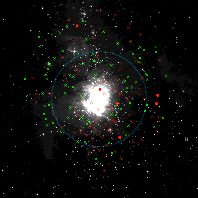
Figure 1: $H$-band 2MASS image showing the spatial distribution of our sample. The field is centered on Trapezium cluster and covers an area of about 0.5°$\times$0.5°. Circles and squares show the fibers allocated to stars with $v\sin i$ larger and smaller than 9.0 km s^-1 (our detection limit; cf. Sect. 2.4), respectively. Crosses indicate sky position to where sky fibers were allocated. Filled symbols mark the position of our most probable binary stars. The circle in the center of the field represents the cluster radius. It is centered on $\Theta^{1}$ Ori and has a radius of about 1 pc (cf. Sect. 3.4.1).

This project has been executed as part of the Science Verification of the Fiber Large Array Multi-Element Spectrograph (flames; Pasquini et al. 2002) attached to the Kueyen Telescope (UT2) at the Paranal Observatory (ESO). Additional observations were obtained with flames GTO observations in Period 76A. Both observing runs were performed with the multi-object GIRAFFE spectrograph in MEDUSA mode. We selected from Hillenbrand (1997) 96 stars with a membership probability given by Jones & Walker (1988) higher than 95%. Their spatial location is shown in Fig. 1, while their position in the HR diagram is shown in Fig. 2. Five stars in our sample, namely, JW50, JW99, JW239, JW669, and JW961 following the Jones & Walker (1988) number, have a mass higher than $\leavevmode\nobreak\ 0.25M_{\odot}$ and $\log T_{\rm eff}>3.5$ K. In the end, 91 targets were selected covering a mass range of $\leavevmode\nobreak\ 0.10-0.25M_{\odot}$ according to Siess et al. (2000), i.e. 35% of the Hillenbrand (1997) sample with $M\leq 0.25M_{\odot}$ (cf. Sect. 3.4.2).

Observations were carried out in 2003 from January 25th to February 3rd (5 hours in 5 nights) and in 2005–2006 from October 15th to January 20th (8.4 hours in 11 nights). Two different GIRAFFE setups were chosen. The first setup, HR14 (resolution $R=28\,300$) covers the range 638.3–662.6 nm containing the H$\alpha$ line. The second one, HR15 ($R=19\,300$), covers the range 659.9–695.5 nm containing the Li i line at 6708 Å. A log of the observations is given in Table 1. In particular, 5 stars (namely JW50, JW99, JW239, JW669, and JW961) were observed only with the lithium set-up.

The GIRAFFE Base-Line Data Reduction Software (girBLDRS; Blecha et al. 2000) was used to reduce the data. Sky subtraction is described in Sect. 2.5.2.

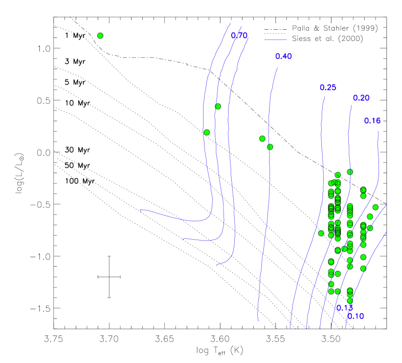
Figure 2: Positions on the HR diagram of the stars included in our sample. Luminosities and effective temperatures (and their mean errors) are taken from Hillenbrand (1997). The Siess et al. (2000) pre-main sequence evolutionary tracks at X=0.703, Y=0.277, and Z=0.020 are also displayed with the labels representing their masses. The Palla & Stahler (1999) birth-line and isochrones (from 1 to 100 Myr) are showed with dash-dotted and dotted lines, respectively.

Table 1: Log of the observations.

$\alpha$	$\delta$	Date	UT	$t_{\rm exp}$	Filter
(°)	(°)	(d/m/y)	(h:m:s)	(s)
83.82747	$-$31.2880	25/01/2003	02:45:19	3600	HR14
83.82750	$-$31.2880	26/01/2003	02:14:47	3600	HR15
83.82762	$-$31.2881	28/01/2003	02:32:05	3600	HR15
83.82766	$-$31.2881	29/01/2003	02:10:41	3600	HR15
83.82763	$-$31.2880	03/02/2003	02:35:43	3600	HR15
83.82731	$-$31.2880	15/10/2005	07:34:36	2820	HR15
83.82730	$-$31.2881	16/10/2005	07:21:02	2820	HR15
83.82730	$-$31.2881	17/10/2005	07:23:30	2820	HR15
83.82739	$-$31.2880	18/10/2005	06:48:58	2820	HR15
83.82729	$-$31.2880	19/10/2005	07:23:02	2820	HR15
83.82725	$-$31.2881	20/10/2005	07:17:21	2820	HR15
83.82730	$-$31.2881	21/10/2005	06:43:18	2820	HR15
83.82731	$-$31.2880	04/11/2005	06:25:09	2820	HR15
83.82747	$-$31.2880	05/11/2005	05:05:07	2820	HR15
83.82718	$-$31.2881	18/01/2006	03:28:53	2820	HR15
83.82707	$-$31.2881	20/01/2006	04:05:22	2054	HR15

2.2 Rotational and Radial Velocity Analysis

Radial velocities ($V_{\rm rad}$) and projected rotational velocities ($v\sin i$) were derived using a cross-correlation of the object spectrum from 660.6 to 696.5 nm against a CORAVEL-type numerical mask (Baranne et al. 1979; Benz & Mayor 1984) based on a M4 stellar spectrum (Delfosse et al. 1998). Regions containing telluric lines and strong photospheric lines (such as the hydrogen lines) were removed from the mask. The cross-correlation function (CCF) can be fairly well fitted by a Gaussian function where the abscissa of its minimum gives the radial velocity and its width, $\sigma_{\rm CCF}$, is related to the broadening mechanisms intrinsic to the stars affecting the photospheric lines convolved by the instrumental profile.

In order to compute $V\sin i$ using $\sigma_{\rm CCF}$, the constants $A$, and $\sigma_{0}$ need to be determined in the expression below:

$$v\sin i=A\sqrt{\sigma_{\rm CCF}^{2}-\sigma_{0}^{2}}\,.$$ (1)

The constant $A$ coupling the differential broadening of the CCF to the $v\sin i$ was determined as described in Melo et al. (2001a), and has a similar value, 1.9, as found by these authors. The width of the CCF of a non-rotating star, $\sigma_{0}$, however could not be determined as in Melo et al. (2001a) due to the lack of calibrators with well determined rotational velocities. Instead the $\sigma_{\rm CCF}$ of the Th-Ar spectrum was used as a proxy for $\sigma_{0}$ (Fig. 3). The caveat is that this determination of $\sigma_{0}$ includes solely the instrumental profile, which is the dominant contributor in the case of low- and mid-resolution spectrographs such as GIRAFFE.

As an example, the CCF for the flames solar spectrum acquired with the same set-up and fiber mode as the stars studied here was computed . Assuming a $v\sin i=2$ km s^-1 for the Sun, we found a $\sigma_{0}=7.1$ km s^-1. Such a difference in the $\sigma_{0}$ would translate to a difference of 1.2 km s^-1 in $(v\sin i)_{\rm min}$ (i.e. the minimum $v\sin i$ we can measure with this GIRAFFE set-up; see cf. Sect. 2.4). Therefore, we adopt $A=1.9$ and $\sigma_{0}=6.62$ km s^-1 as the constants in Eq. 1.

Figure 3: CCF of the Th-Ar emission-line spectrum against a Th-Ar template. The fit gives a $FWHM$ of 15.6 km s^-1.

2.3 $v\sin i$ and $V_{\rm rad}$ errors

Photon noise errors were estimated as in Melo et al. (2001a). The procedure is summarized as follows. A grid of artificially rotated spectra from 5 to 20 km s^-1 was created based on the GIRAFFE solar spectrum. Gaussian noise was added to simulate a $S/N$ varying from 5 to 40. For each point on the grid, 96 spectra were generated. The error of $V_{\rm rad}$ is similar to the error of $v\sin i$, which is given by:

$$\sigma_{v\sin i}\sim\sigma_{V_{\rm rad}}=\frac{1.4\times v\sin i}{S/N}-0.25\,.$$ (2)

For almost all targets several measurements are available. In such cases, the errors quoted in Table 2 are simply based on the scatter of the individual measurements. For four stars (namely, JW99, JW689, JW964, and JW1032) we obtained only one good measurement. In such cases, the errors quoted in Table 2 were computed from the Eq. 2.

2.4 $v\sin i$ detection limit

The smallest $v\sin i$ that can be measured was estimated using Eq. 4 of Melo et al. (2001a). Visual inspection of different lines of Th-Ar shows that the typical $\Delta\sigma_{0}$ is of the order of $1$ km s^-1. To this value, one has to add the typical (external) error ($\sigma_{\rm CCF}^{\rm ext}$) of the measurement of $\sigma_{\rm CCF}$ itself. For stars in our sample with multiple observations the mean rms of $\sigma_{CCF}$ is about 0.7 km s^-1.

Plugging these values into Eq. 4 of Melo et al. (2001a), we find: $(v\sin i)_{\rm min}\la A\sqrt{2\sigma_{0}\epsilon}\sim 9.0$ km s^-1, where $A=1.9$, $\sigma_{0}=6.62$ km s^-1, and $\epsilon=\Delta\sigma_{0}+\sigma_{\rm CCF}^{\rm ext}=1.7$ km s^-1.

2.5 Disk and accretion diagnostics

2.5.1 $\Delta(I_{\rm C}-K)$ excess

The $I_{\rm C}$-band fluxes are least affected by circumstellar activity and typically dominated by photospheric emission, while emission arising from accretion disks is maximized at $K$-band. Hillenbrand et al. (1998) defined a quantity that they used to measure the magnitude of the near-infrared excess:

$$\Delta(I_{\rm C}-K)=(I_{\rm C}-K)_{\rm observed}-0.5A_{V}-(I_{\rm C}-K)_{\rm photosphere}$$ (3)

which represent the difference between the observed $(I_{\rm C}-K)$ color, and the contributions of the reddening and the underlying stellar photosphere. The principal uncertainty in this parameter comes from the photometric error and the time variability of the photometry (Hillenbrand et al. 1998). These authors adopted a value of $\Delta(I_{\rm C}-K)=0.3$ to divide the disk-less stars from the disked ones.

2.5.2 H$\alpha$ line

The width of H$\alpha$ profiles is commonly used as an indicator of accretion in T-Tauri stars. Accreting T-Tauri stars (CTTS) show strong, broad H$\alpha$ profiles whose origin is related to infall of high-velocity material forming their circumstellar disk onto the photosphere (e.g., Hartmann et al. 1994), while weak-line T-Tauri stars (WTTS) show a much narrower H$\alpha$ profile, mostly produced by strong chromospheric activity. Due to differences in the continuum level in the region close to the H$\alpha$ line for different temperatures, no unique value of its equivalent width can be used to distinguish between CTTS and WTTS (Martin 1998). Hence, the threshold for classifying an object as an accretor depends on the spectral type. White & Basri (2003) proposed a full width of H$\alpha$ at 10% of the line’s peak intensity (what they called the 10% width) as a more robust and unified criterion to diagnose stellar accretion regardless the spectral type. Using the presence of veiling as an accretion criterion, they proposed that a 10% width larger than 270 km s^-1 indicates the star is accreting, and therefore can be classified as a CTTS. Using physical reasons and empirical findings, Jayawardhana et al. (2003) adopted 200 km s^-1 as the accretion cutoff for the very low-mass regime (down to the limit of hydrogen burning). This value corresponds to a mass accretion rate of about $10^{-10}M_{\odot}$ yr^-1. Measurements of 10% widths are advantageous over optical veiling and H$\alpha$ equivalent width measurements because they can be extracted over a short wavelength range, do not depend on the underlying stellar luminosity, and do not depend on the availability of a comparison template (White & Basri 2003).

In order to be able to compute the 10% widths for all fibers (i.e., stellar and sky spectra), we first fitted and then subtracted the continuum around 654 nm up to 660 nm. The continuum subtracted spectra were then normalized by their highest intensity. Some examples of the final spectra used to computed the 10% widths are shown in Fig. 4.

Figure 4: H$\alpha$ velocity profiles for five different objects of the ONC and one sky position. The H$\alpha$ 10% intensity is showed with a dashed line.

The H$\alpha$ profiles in the ONC are known to be strongly contaminated by the nebular emission. However, at our spectral resolution, the sky emission lines are much narrower than the profile expected for an accreting star (Stassun et al. 1999). As an additional check of the level of contamination, we compared the 10% widths measured for the object fibers and those allocated to sky positions. As we can see in Fig. 5, sky fibers show a rather narrow distribution of 10% widths in the range of 50-70 km s^-1. In contrast, stars have values from 50 to 250 km s^-1. It is worth noticing that, according to White & Basri (2003) criterion, none of the ONC stars studied here is accreting. This will be better discussed in Sect. 4.

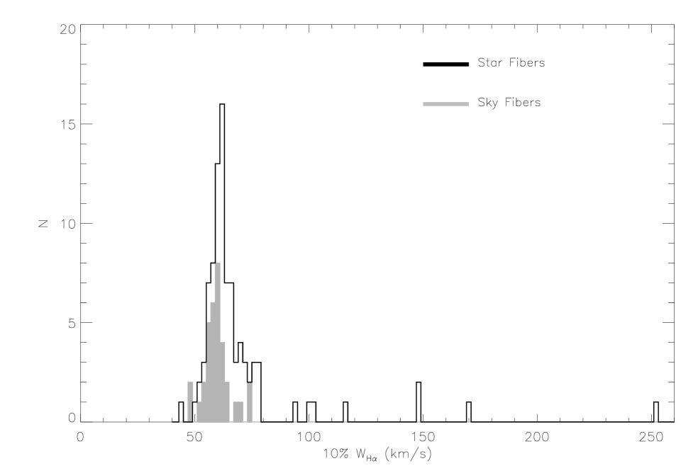
Figure 5: Distribution of 10% widths. Sky emission distribution is shown with the filled grey histogram whereas the objects are displayed in continuous black line. Stars showing 10% widths below $\sim 70$ km s^-1 are likely to be dominated by the sky emission.

2.5.3 [3.6]$-$[8.0] $\mu$m flux

The Orion Molecular Cloud was surveyed with the Spitzer Space Telescope as part of GTO program (Megeath et al. 2008). The IRAC@Spitzer mid-infrered bands can be used as circumstellar disk diagnostics (Rebull et al. 2006). In particular, the color index based on the two most widely separated bands, namely 3.6 $\mu$m and 8 $\mu$m, is a very useful method for distinguishing disk and non-disk candidates, with [3.6]$-$[8.0]=1 the boundary between disk and non-disk candidates (Rebull et al. 2006).

2.5.4 Ca ii infrared triplet

As pointed out by Hillenbrand et al. (1998), the Ca ii infrared triplet ($\lambda\lambda$8498, 8542, 8662) can be used to explore the presence of accreting disks. The triplet emission features exhibit narrow and broad components, which seem to show a correlation with spectral veiling measured at optical wavelengths, implying a correlation with the mass-accretion rate. The authors analyze the behavior of the equivalent widths (EWs) of the strongest level (i.e. $\lambda$8542) in their sample of low-mass ONC stars. According to their convention, stars are supposed to have accretion disks if the sum of the EWs of the broad and narrow components is filled or in emission ($W_{\rm CaII}=0\pm 1$ Å). They emphasize that definite conclusions regarding either disk frequency or accretion properties based on the Ca ii infrared lines await studies capable of separating photospheric absorption, narrow-component emission, and broad-component emission. In Table 2 the column $W_{{Ca\textsc{ii}}}$ lists the EWs of our targets taken from Hillenbrand et al. (1998), where values of 0.0 indicate that neither emission nor absorption features were apparent from visual inspection of the spectrum.

3 Results and discussion

3.1 Radial velocities and spectroscopic binaries

A histogram of radial velocity measurements for the sample of low-mass stars is shown in Fig. 6. The Gaussian fit of the distribution yields a mean $V_{\rm rad}$ of 24.87 km s^-1 and $\sigma_{V}{}_{\rm rad}$ of 2.74 km s^-1 in very good agreement with the typical values found in the literature (see, e.g., Stassun et al. 1999; Alcalà et al. 2000; Covino et al. 2001; Rhode et al. 2001). Our radial velocities confirm the membership of all stars in the sample, as expected, since the targets have been selected based on the membership probability given by Jones & Walker (1988).

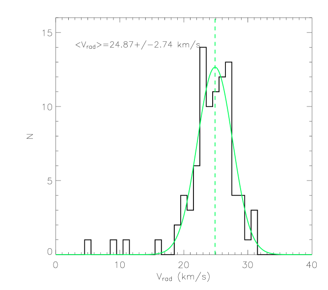
Figure 6: Radial velocity distribution for our sample of stars with $M<0.25M_{\odot}$. For the most probable binaries we plot the mean values of the two components (Table 2). The Gaussian fit of the distribution yields a mean $V_{\rm rad}$ of 24.87 km s^-1 (with a $\sigma_{V}{}_{\rm rad}$ of 2.74 km s^-1), which is fully consistent with the membership in the ONC (e.g., Stassun et al. 1999).

Among the 96 stars observed, 6 (JW50, JW54, JW239, JW276, JW500, and JW840) show a double-lined CCF (Fig. 7). Three of these, JW50, JW239, and JW840, were already classified as binaries by Jones & Walker (1988) and Tobin et al. (2009), and two of them (namely JW50 and JW239) have $M>0.25M_{\odot}$ (Fig. 2). For our most probable low-mass binaries we show in Fig. 6 an average of the radial velocities of the two components. The $V{}_{\rm rad}$ values for both the components and their mean values are also listed in Table 2 for all the sample.

Future radial velocity follow-up of such targets would help to solve their orbits and to determine the circularization period in this mass range which can bring interesting information about the frequency of spectroscopic binaries and internal dissipation mechanisms of angular momentum related to the convective motion within the stars (e.g., Melo et al. 2001b).

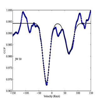
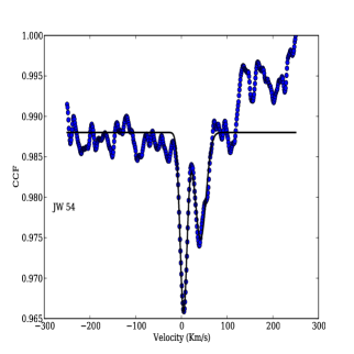
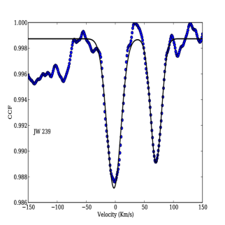
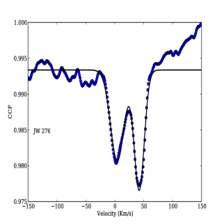
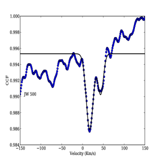
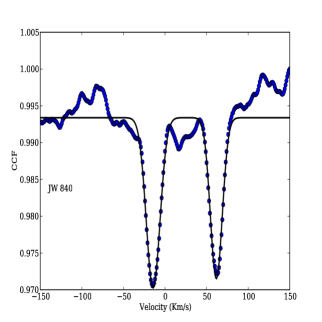
Figure 7: Double-lined CCF profiles for our most probable binary stars.

3.2 Rotation period and radius from $v\sin i$

We considered the low-mass stars having both $v\sin i$ (Fig. 8) above our detection limit of 9 km s^-1 as well as radii determined by Hillenbrand (1997). For these 57 objects we computed $P_{\rm rot}/\sin i=2\pi R/v\sin i$. For the binary stars, we considered $v\sin i$ values of the first component listed in Table 2. These periods distribute according to a unimodal distribution peaked around $P_{\rm rot}/\sin i=3-5$ day/rad (Fig. 9). Considering a statistical correction of $<\sin i>=\pi/4$ (cf. Sect. 3.3), our period distribution seems to have a peak at $\sim 2.4-3.9$ days, while with our $<\sin i>=0.61$ (cf. Sect. 3.3) the peak is around $1.8-3.1$ days. This result is in agreement with previous ones present in the literature for stars with $M<0.25M_{\odot}$ (see, e.g., Herbst et al. 2007, and references therein). Namely, whereas stars with $M>0.25M_{\odot}$ present a bimodal rotational period distribution with two peaks near 2 and 8 days, low-mass stars ($M<0.25M_{\odot}$) show a unimodal distribution peaked near 2 days.

Combining our $v\sin i>9$ km s^-1 values with the rotation period measured by Herbst et al. (2002) we can constrain the minimum stellar radii for 23 low-mass stars. Taking into account the relationship $R\sin i=P_{\rm rot}v\sin i/2\pi$, we find our $R\sin i$ ranges from 0.7 to 1.2 $R_{\odot}\cdot$rad, with a distribution peaked to around $0.9-1.5R_{\odot}$ if we consider $<\sin i>=\pi/4$, and $\sim 1.1-2.0R_{\odot}$ for our $<\sin i>=0.61$ (cf. Sect. 3.3). The Hillenbrand (1997)’s radii for the same stars show a peak around $1.3-1.4R_{\odot}$.

Figure 8: $v\sin i$ distribution for our low-mass stars. Our $v\sin i$ limit of 9 km s^-1 is shown with a dotted line.

Figure 9: Rotational period distribution obtained with our $v\sin i>9$ km s^-1 values (namely, 57).

3.3 $v\sin i$ and $v_{\rm eq}$

We compared $v\sin i$ with equatorial velocities $v_{\rm eq}=2\pi R/P_{\rm rot}$ calculated adopting the radii and rotational periods by Hillenbrand (1997) and Herbst et al. (2002), respectively (Fig. 10). For stars with $v\sin i<9$ km s^-1 detection limit arrows are plotted. The solid and dashed lines mark $v\sin i=v_{\rm eq}$ and $v\sin i=(\pi/4)v_{\rm eq}$, respectively. Similar to what was found by Rhode et al. (2001), almost all our 34 stars fall below the $v\sin i=(\pi/4)v_{\rm eq}$ line, indicating that the average $\sin i$ value we measure is lower than the expected value. We computed the mean $\sin i$ considering the stars with $v\sin i>9$ km s^-1, finding $<\sin i>=0.61\pm 0.04$, very close to previous values (see, e.g., Rhode et al. 2001, and references therein), but significantly lower than the value of $\pi/4\sim 0.785$ expected for a random oriented distribution of stellar rotation axes (Chandrasekhar & Munch 1950). This departure has been also observed in previous studies of PMS, and a number of explanations, including real physical phenomena, and systematic errors in astrophysical quantities ($v\sin i$, $L$, $T_{\rm eff}$, $P_{\rm rot}$) have been invoked by several authors. Rhode et al. (2001) explored, in their sample of $0.1<M<2.5M_{\odot}$ stars, all these possibilities finding that the correct $\sin i$ value is produced assuming that the effective temperatures have been underestimated by 400–600 K. Trying to resolve this problem is beyond the scope of this work. We would only stress that the radii computations of Hillenbrand (1997) were based on a distance of 470 pc, while recent determinations estimate a distance to ONC of 414 pc (Menten et al. 2007). This leads to $R$, $P_{\rm rot}/\sin i$, and $v_{\rm eq}$ 12% smaller than we find, and a mean $\sin i$ of 0.683, i.e. closer to the statistics value. This means our findings are also partially linked to the distance determinations.

Moreover, Fig. 10 shows there is a correlation between $v\sin i$ and $v_{\rm eq}$, demostrating, as pointed out by Rhode et al. (2001), that the periodicity of our T Tauri stars is caused by the rotation of stars with spotted photospheres.

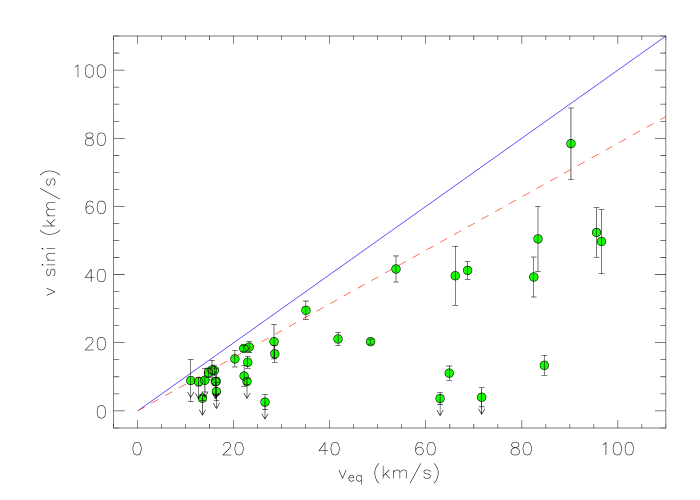
Figure 10: $v\sin i$ versus $v_{\rm eq}$. The continuous and dashed lines represent the equations $v\sin i=v_{\rm eq}$ and $v\sin i=(\pi/4)v_{\rm eq}$, respectively. The arrows refer to our detection limit of 9 km s^-1.

3.4 Correlations with $v\sin i$

Our $v\sin i$ results are given in Table 2. Of the 91 stars observed with $0.10<M<0.25M_{\odot}$, 4 stars are bona-fide spectroscopic binaries. The binary stars will be marked with different symbols in the following plots since tidal effect may be influencing their surface rotations. Since the $v\sin i$ values of the binary system components are very similar to each other, we decided to plot only the first component listed in Table 2. Finally, 34 stars have $v\sin i$ less than or equal to our limit of 9 km s^-1.

3.4.1 Are stars rotating close to break-up velocity?

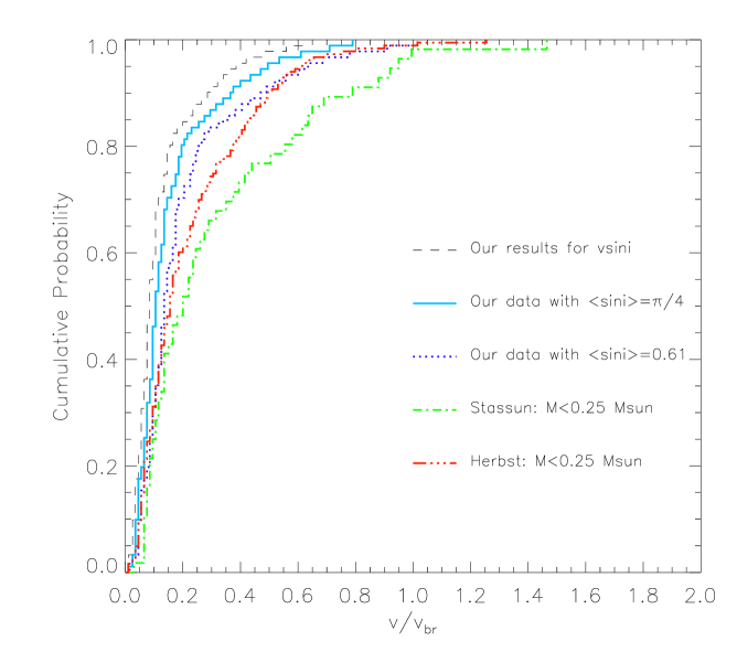
Figure 11: Cumulative distribution of equatorial velocities normalized to break-up velocity. Our sample (dashed, continuous, and dotted lines) is compared to the Stassun et al. (1999) low-mass sample (dash-dotted line) and to the Herbst et al. (2002)’s low-mass sample (dot-dot-dot-dashed line).

In Fig. 11 we show the cumulative distribution normalized to the break-up velocity $v_{\rm br}=\sqrt{GM/R}$ (where $G$ is the gravitational constant) for our low-mass stars. The break-up velocities from our stars were computed using the radii $R$ and masses $M$ taken from Hillenbrand (1997). We compare our results with the $v/v_{\rm br}$ values derived by Stassun et al. (1999) for $M\leq 0.25M_{\odot}$ and with the values obtained considering the $P_{\rm rot}$ derived by Herbst et al. (2002) and mass and radii taken from Hillenbrand (1997) in the same low-mass regime.

We show with different lines our results obtained considering $v\sin i$ (without the $\sin i$ correction) and the values we obtain for our $\sin i$ mean value of 0.61 and the statistical value of about 0.785 expected for a random oriented distribution of stellar rotation axes. A visual inspection suggests that our distributions are very different from the Stassun et al. (1999) findings. While 23% of the 56 Stassun et al. (1999)’s low-mass stars are rotating faster than $0.5v_{\rm br}$, only four stars (namely JW122, JW168, JW530, and JW964) in our sample of 91 stars seems to exceed the $0.5v_{\rm br}$ limit when we consider $<\sin i>=\pi/4$. This number obviously increases to 8 if we consider our $<\sin i>=0.61$. Similar results are found for the 183 low-mass stars of the Herbst et al. (2002)’s sample, where the percentage of stars with $v/v_{\rm br}\geq 0.5$ is about 10%. Thus, we can definitely assert that in our sample, no star is rotating close to the break-up velocity estimated for its mass and radius. Excluding effects due to mass selection effects of the samples, an effect linked to the spatial segregation cannot be excluded, because the stellar population observed by Stassun et al. (1999) spans a big area of $40^{\prime}\times 80^{\prime}$ centered on the Trapezium in ONC, while our stars are localized in an smaller area of $20^{\prime}\times 24^{\prime}$. Also the stars of Herbst et al. (2002) are localized in a smaller area ($33^{\prime}\times 34^{\prime}$). In particular, as shown in Fig. 1, about 62% of our sample is almost inside the circle with radius equal to the so-called cluster radius ($R_{\rm cluster}$; Hillenbrand 1997) where Rodriguez-Ledesma et al. (2009) find an indication of higher $P_{\rm rot}$ compared to the stars outside $R_{\rm cluster}$. This could indicate objects closer to the Trapezium center tend to rotate on average slower than the outer ones. An inspection of the Stassun et al. (1999)’s $P_{\rm rot}$ data seems to indicate an almost flat distribution for radii smaller than $R_{\rm cluster}$ and the hint of a peak at low $P_{\rm rot}$ for radii bigger than $R_{\rm cluster}$. With our smaller sample, we are not able to reach any successful conclusion. We would need more stars and/or $v\sin i$ measurements for all their stars. As a consequence, we caution the reader about this issue.

We also computed the Kolmogorov-Smirnov (KS) probability (Press et al. 1992) that the our arrays of data obtained with $<\sin i>=\pi/4$ and the Stassun et al. (1999)’s values for low-mass stars are drawn from the same distribution. We find that the KS probability that these data were drawn from the same distribution is only of 0.04%. A value of 0.5% is obtained considering the stars of Stassun et al. (1999) with $M<0.25M_{\odot}$ locatized in the same spatial region of our sample. This comparison shows that, at least as far as our data is concerned, there is not a fast rotator population in the mass regime covered by our data.

3.4.2 Is there any evidence supporting disk-locking?

One of the well known implications of the disk-locking scenario is that slowly rotating stars should have accreting disks around them while rapidly rotating stars should not. In fact, this picture has been supported over the years in many different papers (e.g., Edwards et al. 1993; Bouvier et al. 1993; Choi & Herbst 1996; Herbst et al. 2001; Rebull et al. 2002).

In particular, if the diagnostics we use here ($\Delta(I_{\rm C}-K)$ excess, 10% H$\alpha$ width, [3.8]$-$[8.0], and Ca ii infrared triplet) and rotation are correlated, in the sense that slow rotators are more likely to show excess and variability, this is evidence in support of the disk-locking paradigm. As pointed out recently by Irwin & Bouvier (2009), this means that the population of slowly-rotating stars should show the presence of a disk (e.g., mid-IR excess) or of active accretion (i.e. be CTTS), whereas the rapidly-rotating stars should not have disk, or have recently-dissipated disks, and not be active accretors (i.e. WTTS). Rebull et al. (2006), analyzing Spitzer mid-IR data for about 900 stars in Orion in the mass range $0.1-3M_{\odot}$ find that slowly-rotating stars are indeed more likely to posses disks than rapidly-rotating stars. However, they also find a puzzling population of slow-rotating stars without disks. This result has been also confirmed subsequently (e.g., Cieza & Baliber 2007).

In Fig. 12 we plot our $v\sin i$ measurements divided by the radii as a function of the near-infrared color excess $\Delta(I_{\rm C}-K)$ given by Hillenbrand et al. (1998) and which is taken as an inner disk tracer, because it quantifies the magnitude of the $K$-band excess above the photospheric level. Negative values of $\Delta(I_{\rm C}-K)$ are attributed by the authors to photometric variability or to errors either in photometry or in spectral types. The vertical line sets the limit of $\Delta(I_{\rm C}-K)$=0.3 proposed as the dividing line between disk-less and disked stars (Hillenbrand et al. 1998). It is clear the difference in the rotational behavior between stars with disk ($\Delta(I_{\rm C}-K)>0.3$) and those without disk ($\Delta(I_{\rm C}-K)<0.3$): while for disk-less stars the rotation rates expand over a large range possibly indicating different time-scales for the unlocking, disked stars mostly present low rotation rates, apart from JW172. The presence of substantial numbers of slow-rotating stars with little or no excess could indicate they may have just recently cleared their disks and have not yet spun up in response to contraction on their way to the ZAMS. In order to assign a confidence level to our result, a one-side 2$\times$2 Fisher’s exact test was used (Agresti 1992). We choose the division between disk-less and disked stars ($\Delta(I_{\rm C}-K)=0.3$) and the division at $v\sin i/R=1.5$ rad/day between slow and fast rotators. We find a p-value of 0.094 as chance that random data would yield this trend, indicating a probability of correlation of 90.6%.

Concerning Orion, Stassun et al. (1999) have challenged the disk-locking scenario claiming no correlation between rotation and infrared properties related to circumstellar disks. The issue was re-examined by Herbst et al. (2002) using the $I_{\rm C}-K$ color excess derived by Hillenbrand et al. (1998) as a disk tracer and their own rotation measurements. They found that the mean value of $\Delta(I_{\rm C}-K)$ for the rapidly rotating sample (i.e., rotation period shorter than 3.14 days) is of 0.17 mag, whereas for the slowly rotating sample (i.e., rotation period longer than 6.28 days) this value rises to 0.55 mag well above the limit of $\Delta(I_{\rm C}-K)$=0.3. The trend observed in Fig. 12 is in agreement with the results reported by Herbst et al. (2001, 2002).

According to the disk-locking theory, a star is thought to be anchored or locked to its disk via its magnetic field that threads the circumstellar disk. Accretion of disk material occurs along the magnetic field lines. Thus, correlations between accretion indicators such as H$\alpha$ equivalent width or veiling index and rotation are expected (e.g., Hartigan et al. 1995; Hillenbrand et al. 1998). Sicilia-Aguilar et al. (2005) carried out a careful analyses of the H$\alpha$ profiles for a sample of 237 members of the ONC. They show that although the distribution of $(I_{\rm C}-K)$-excess for CTTS and WTTS overlap, a $(I_{\rm C}-K)$-excess of 0.5 can be taken as a trustful criteria to distinguish between CTTS and WTTS. As in Herbst et al. (2002), Sicilia-Aguilar et al. (2005) also found evidence for a different behavior in rotation between the CTTS and WTTS in line with that predicted by the disk-locking scenario.

As already pointed out in Sect. 2.5.2, if the 10% width criterion suggested by White & Basri (2003) is used to trace accretors, none of the stars in our sample is actually accreting. In Fig. 13 we plot again the projected angular velocity as a function of the measured 10% widths. The vertical line marks the maximum value of 10% width measured in our sky spectra (at $\sim 76$ km s^-1). Therefore, stars with a 10%-width less than this value are likely to be dominated by the sky emission. We promptly see that only 8 stars appear clearly to the right side of the vertical line. Two of them (JW937 and JW1036) show color excess $\Delta(I_{\rm C}-K)>0.3$. The other 4 slowly-rotating stars (JW52, JW296, JW559, and JW574) are sligthly on the right side of the vertical line, and with their values of $\sim 77-79$ km s^-1 seem to be not highly influenced by the sky fibers (Fig. 5). Thus, even if all these objects are taken as bona-fide accretors, we can safely state that essentially only a fraction of about 14% are accretors in our sample of $0.10-0.25M_{\odot}$, which is lower than the range 61–88% obtained by Hillenbrand et al. (1998) and 40–80% obtained by Sicilia-Aguilar et al. (2005). We do not believe this is due to an effect of sample selection, because our targets represent about 35% of the Hillenbrand et al. (1998) sample with $0.10\leq M\leq 0.25M\odot$, available $\Delta(I_{\rm C}-K)$, and membership probability higher than 95%. Moreover, our sample is well sampled in $\Delta(I_{\rm C}-K)$. In particular, considering the range $0.2<\Delta(I_{\rm C}-K)<0.5$ suitable as disk diagnostics, our sample represents about 25% of the Hillenbrand et al. (1998) targets. Thus, in order to better understand our results, we considered the Sicilia-Aguilar et al. (2005) sample in the low-mass range $0.10-0.25M_{\odot}$, and we found a percentage of accretors of 13–26%, which is more consistent with our findings. Thus, our results seem to be explained by assuming that low-mass stars are by percentage less active accretors than higher-mass stars. Relationships between accretion rates and mass of the central object have been investigated by several authors (see, e.g., the case of $\rho$ Ophiucus, where Natta et al. (2006) find $\dot{M}_{\rm acc}\propto M_{\star}^{1.8}$ in $0.03-3M_{\odot}$ stars).

Contrary to the case of more massive stars where disk-locking is supported by rotation-color excess and rotation-accretion correlations (Herbst et al. 2002; Sicilia-Aguilar et al. 2005), the lack of strong concordance between Fig. 12 and Fig. 13 is intriguing. Dividing the data in Fig. 13 in four boxes by $v\sin i/R=1.5$ rad/day and $10\%W_{\rm H\alpha}=76$ km s^-1, the one-sided 2$\times$2 Fisher’s exact test leads to a p-value of 0.936, implying a probability of correlation of only 6.4%.

Herbst et al. (2002) showed evidence in the ONC for a clear difference in the rotation behavior for stars below 0.25$M_{\odot}$ and those more massive than 0.25$M_{\odot}$ and this was also observed by Lamm et al. (2005) for the older cluster NGC 2264. When the angular velocities of both groups are compared (Fig. 19 of Herbst et al. 2002), the distribution of angular velocity for the more massive stars is highly concentrated in one bin only at $\omega\sim 1$ rad day^-1. This is in contrast to the angular velocity distribution for stars $M<0.25M_{\odot}$, which spread out essentially between $\omega\sim 1-4$ rad day^-1. A possible interpretation given by Herbst et al. (2002) for this difference is that low-mass stars remained locked to their disks for a shorter period of time as compared to the more massive group. Thus, the distribution seen in ONC for the low-mass stars is already the result of the spin-up of a group of unlocked stars. Similar findings are reported by Lamm et al. (2005) for NGC 2264.

Fig. 13 suggests that indeed almost none of the stars observed here are locked to their disks. Are Fig. 12 and Fig. 13 in contradiction? In other words, can unlocked stars (i.e., non accreting stars) still hold a rotation-color-excess relation? In Fig. 14 we schematically describe the evolution of a rotation ($\omega$) and color-excess (disk) diagram. Disk-locking operates for a fixed duration of time long enough to establish a rotation-color-excess relation. At a time $t_{0}$ all stars are unlocked (Fig.14a). As the contractions proceed all stars (slow and fast rotators) spin-up by a factor proportional to the value $(R_{t_{0}}/R_{t_{1}})^{2}$. Although color-excess diminishes due to disk dissipation, a rotation-color-excess relation is even stronger since the spin-up depends on $\omega_{0}$. Eventually disks disappear completely and we end up with a large spread in rotation as observed in the ZAMS clusters. Therefore, our Fig. 12 and Fig. 13 indicate that: i) the low-mass stars in the ONC are not currently locked, but ii) the rotation-color-excess relation suggests that these stars were locked once.

From Fig. 15, the EW of $\lambda$8542 Ca ii seems to have values indicating the presence of broad (also of the order of one hundred km s^-1) Ca ii line emission or a partially filled-in line, phenomena associated with an accreting disk, for low $v\sin i/R$, while for higher rotational velocities there is almost no evidence of line emission or filling-in. Hillenbrand et al. (1998) conclude that stars with higher accretion rates should exhibit detectable Ca ii emission above continuum levels, while stars that lack accretion disks should show net Ca ii absorption with absorption equivalent widths $W_{{Ca\textsc{ii}}}>1$. Possible explanations of the observed descrepancy between Fig. 12 and Fig. 15 could include the difficulty of measuring $W_{{Ca\textsc{ii}}}$ for very late-type stars due to a low spectral resolution and to contrast effects. Moreover, as shown by Batalha et al. (1984), one expects a strong correlation between optical veiling (i.e., accretion) and the broad component of the Ca ii line. In addition, at the spectral resolution used by Hillenbrand et al. (1998), the broad component and the narrow component of this line always appear blended. Finally, small emission-line equivalent widths are more difficult to detect for low-mass stars because of the photospheric calcium line and the strong TiO bands. Thus, we think this diagnostic at present is not reliable and should be revisited using higher spectral resolution. Nevertheless, the fact that indeed most of the stars with broader Ca ii line are those with $v\sin i<9$ km s^-1 (our detection limit) prevent us in connecting this diagnostic to the disk-locking scenario.

Fig. 16 shows the [3.8]$-$[8.0] color versus $v\sin i/R$ for the stars in common with Rebull et al. (2006). The number of stars is very limited (13), so it would seem conclusions could not be drown. We notice, however, that all the stars with strong color excess (i.e. above [3.8]$-$[8.0]=1) are slow rotators, and 7/10 have only detection limit $v\sin i$ measurements. Applying the one-sided Fisher’s exact test, after the division of the plot at $v\sin i/R=1.5$ km s^-1 and [3.8]$-$[8.0]=1, we find a p-value of 0.038, which supports an association between the data at the $\sim$96% confidence level (i.e. more than 2 sigma) even though the numbers of measurements is small. Edwards et al. (1993) and Rebull et al. (2006) found similar results and speculated that the long-period diskless objects have recently released their disks (within a few hundred thousand years).

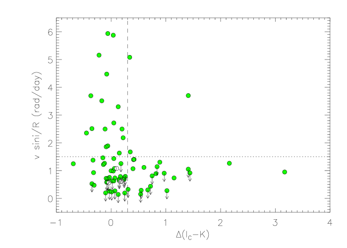
Figure 12: Rotation against disk tracers. Rotational velocity as a function of the near infrared excess. A drop in the rotation rate is clearly seen for stars with a circumstellar disk (i.e., $\Delta(I_{\rm C}-K)>0.3$). The empty circles represent the position of the most probable binaries. The dotted line marks the division we considered for the Fisher’s test.

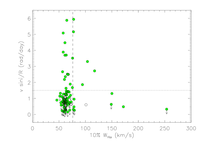
Figure 13: Rotation against accretion tracers. Rotational velocity as a function of the full width of the H$\alpha$ line at 10% of its intensity. The empty circles represent the position of the most probable binaries. The dashed line marks the maximum value of 10% $W_{\rm H\alpha}$ measured in our sky spectra, while the dotted line marks the division we considered for the analysis of the Fisher’s test.

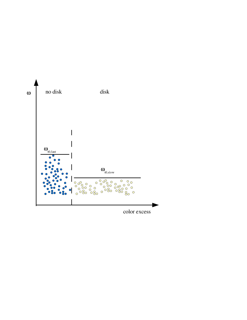
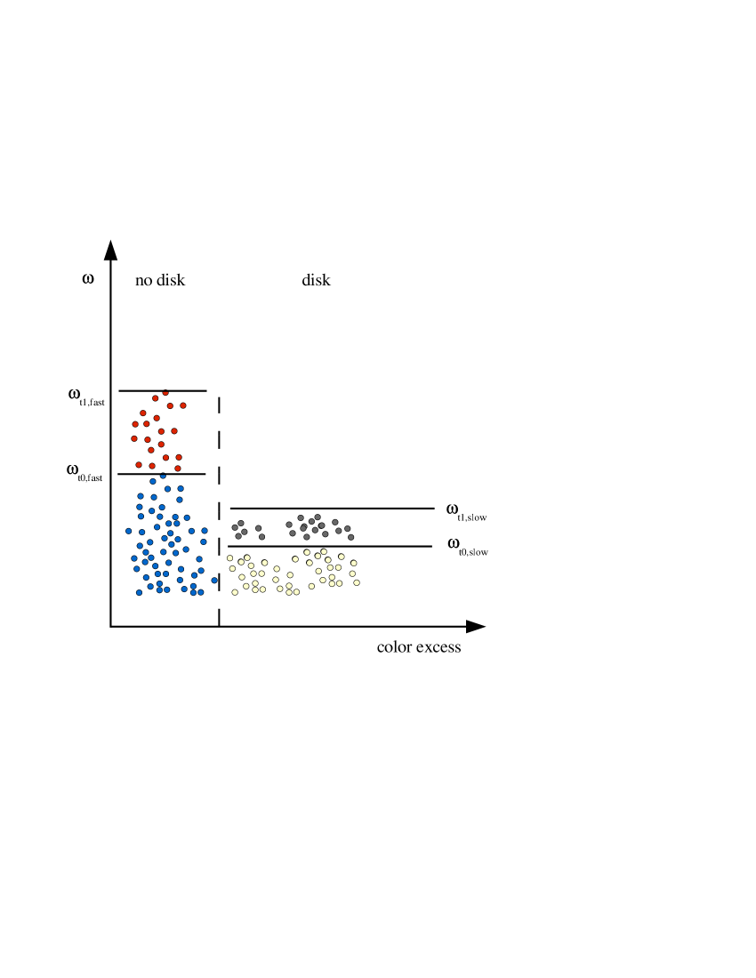
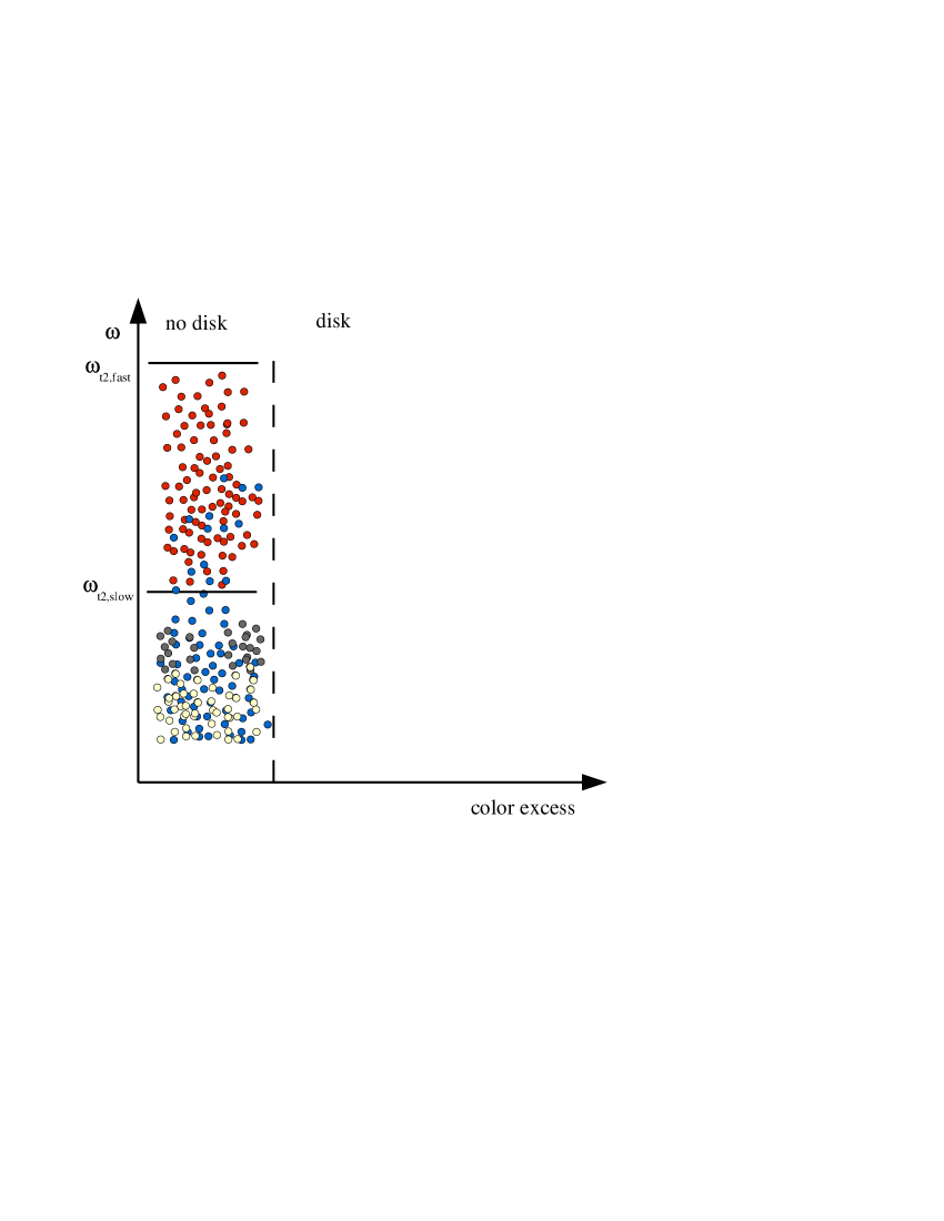
Figure 14: Schematic view of the diagram angular rotational velocity versus color excess for three different evolutive times.

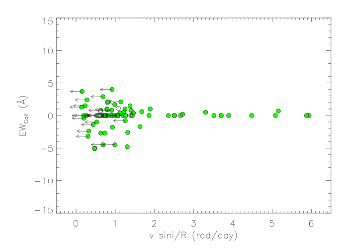
Figure 15: Ca ii $\lambda$8542 equivalent width (disk tracer) as a function of $v\sin i/R$. The possible relation between disk frequency and rotation is not visible. The empty circles represent the position of the most probable binaries.

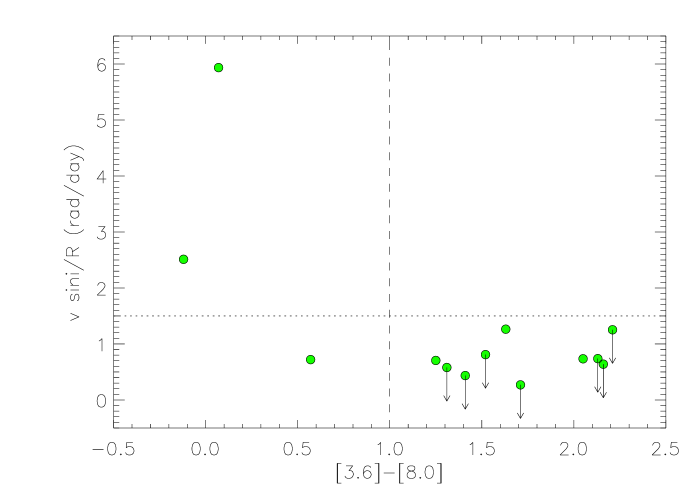
Figure 16: Rotation against disk tracers. [3.8]$-$[8.0] as a function of $v\sin i/R$. A possible relation between disk frequency and rotation is visible. The vertical line marks the boundary between disk and non-disk candidates, while the orizontal line marks the division for the Fisher’s test.

3.4.3 Rotation and X-ray activity

Based on X-ray measurements carried out by Chandra in the ONC, Feigelson et al. (2003) have shown that the ONC stars have stronger X-ray emission than main-sequence stars with similar rotation periods and that the strong anti-correlation between X-rays and period observed for main-sequence stars is not seen for the ONC population. Instead, they claim that a marginal correlation (i.e., X-rays increasing with the rotation period) is seen in the data. In Fig. 17 we show the logarithm of the ratio $L_{\rm X}/L_{\rm bol}$ of total band X-ray to bolometric luminosity as a function our $v\sin i$ divided by the theoretical radii for the stars in our sample in common to Feigelson et al. (2003). In spite of the scatter seen in the X-rays levels, the X-rays-rotation relation seems to be flat, suggesting that all stars in the sample are close to a “saturated regime” down to our detection limit in $v\sin i$. Recently, Mohanty & Basri (2003) find that the chromospheric H$\alpha$ activity saturates at $\sim 3$ km s^-1 and at $\sim 10$ km s^-1 for M4-M5- and for M5.5-M8.5-field dwarfs, respectively, while the X-ray activity saturates at $\sim 3$ km s^-1 for early M stars. Considering their results and our $v\sin i$ detection limit, the unsaturated part of the possible activity-rotation relation is clearly beyond our sensitivity.

For very low-mass stars (late M and L spectral types), the rotation-activity relationship is not really known, because their low rotation velocity is often below the detection limits (e.g., Stauffer et al. 1997; Mohanty & Basri 2003; Messina 2007).

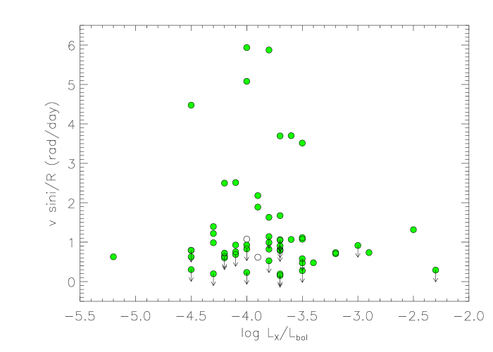
Figure 17: Rotation versus activity for our stars. In spite of the scatter seen in the X-rays levels, the data suggest that all stars in the sample are close to a saturated regime down to our detection limit in $v\sin i$. The empty circles represent the position of the most probable binaries.

4 Summary and Conclusion

We have presented the results of a search for evidence of the disk-locking scenario as a mechanism for angular momentum depletion in a region centered on the Trapezium and extending beyond the ONC. We use our spectroscopic observations to derive radial velocities, and rotation rates, and to identify possible stars undergoing active disk accretion. In addition, we use IR photometric data from the literature to identify those stars possessing circumstellar disks. The results for our most probable single low-mass ($0.10<M<0.25M_{\odot}$) stars can be summarized as follows.

1. We find a correlation between $v\sin i$ and $v_{\rm eq}$ confirming that the observed modulation is due to migrating inhomogeneities (Rhode et al. 2001).

2. We measure an average $\sin i$ lower than the mean value expected for a random distribution of stellar rotation axes, as already found by other authors (see, e.g., Rhode et al. 2001).

3. We do not find evidence for a population of fast rotators close to the break-up velocity. This supports the suggestions by Hartmann (2002) that the timescale for angular momentum loss is comparable to the age of the ONC stars, so that disk braking may not be completely effective, at least among the lowest mass stars.

4. From the $v\sin i-\Delta(I_{\rm C}-K)$ relation we find: 1) slow-rotators with disks, where the low $v\sin i$ is due to the coupling between star and disk; 2) slow-rotators without disks, as found by Rebull et al. (2006) and corresponding to stars that are losing their disks, and hence continuing to rotate slowly for some time, but gradually spinning-up as they contract towards the ZAMS; 3) fast rotators without disks, where stars get free from their disks becoming fast rotators; 4) almost no fast rotators with disks (with the exception of a single star).

5. From the $v\sin i-10\%$-width relation, we do not find stars are actually accreting, but we argue that all non-accretors are either low or fast rotators, as found by Jayawardhana et al. (2006) in $\eta$ Cha and TW Hydrae ($\sim 6-8$ Myr).

6. The Ca ii line indicates possible phenomena associated with an accreting disk in stars around our $v\sin i$ limit, but we are very cautious about this diagnostic at present. A revision at higher resolution to arrive at a firmer conclusion.

7. The few [3.8]$-$[8.0] colors available for our sample show that all stars with color excess are slow rotators.

8. There is no clear relation between rotation and X-ray activity essentially due to the fact that all of our stars occupy “saturated regime”.

All these results are consistent with the following picture:

1. very low-mass stars in our sample are not locked now, but they were locked in the past;

2. the percentage of accretors seems to scale inversely to the mass of the stars.

Table 2: Our sample.

JW	$I_{\rm C}$	$V-I_{\rm C}$	$\log T_{\rm eff}$	$R$	$M$	Spec. Type	$\Delta(I_{\rm C}-K)$	$W_{\rm CaII}$	10% $W_{\rm H\alpha}$	$v\sin i$	$V_{\rm rad}$	$\log\frac{L_{\rm X}}{L_{\rm bol}}$	$P_{\rm rot}$	[3.6]$-$[8.0]	Source
	(mag)		(K)	($R_{\odot}$)	($M_{\odot}$)			(Å)	(km s-1)	(km s${}^{-1})$	(km s-1)		(days)
38	15.6	3.73	3.494	1.48	0.14	M5	$-$0.35	$-$1.0	62.2	$<$9.0	24.80$\pm$0.28				1;7,8
43	15.8	3.73	3.483	1.27	0.11	M5.5	$-$0.33	1.5	64.2	14.1$\pm$2.6	27.21$\pm$0.69				1;7,8
48	15.5	4.60	3.471	2.49	0.14	M6	$-$0.69	1.0	62.1	25.0$\pm$7.7	27.10$\pm$4.66				1;7,8
50∗,a	11.7	1.75	3.602	3.46	0.34	K1e,G-Ke,K7.3	1.37	$-$14.6		20.9$\pm$1.2	$-$20.87$\pm$1.20				1,2,3;7,8
										23.8$\pm$1.4	66.38$\pm$1.40
											22.75$\pm$1.80b
52	14.6	3.64	3.494	2.25	0.15	M5	$-$0.03	0.0	79.1	$<$9.0	24.43$\pm$0.54				1;7,8
54a	15.3	3.58	3.494	1.57	0.14	M5	$-$0.04	0.0	62.2	$<$9.0	4.80$\pm$0.25				1;7,8
										18.8$\pm$1.1	42.01$\pm$1.07
											23.40$\pm$1.10b
70	15.3	3.89	3.494	1.96	0.14	M5	$-$0.35	0.0	65.8	39.7$\pm$8.7	19.38$\pm$4.72	$-$4.1	1.50	$-$0.12	1;9,7,8,13
99∗,c	13.1	2.51	3.562	2.92	0.24	M1	0.50	1.4		16.9$\pm$0.9	66.34$\pm$0.93		1.70	0.57	1;9,7,8,13
110	16.6		3.483	0.78	0.09	M4-7		0.0	61.9	$<$9.0	28.01$\pm$0.96	$-$3.7			1;7,8
118	14.8	3.09	3.483	1.79	0.13	M5.5	$-$0.32	0.0	59.6	13.4$\pm$3.0	24.49$\pm$0.35	$-$4.0	1.07		1;9,7,8
120	14.3	3.01	3.500	1.80	0.16	M4.5	$-$0.06	1.0	71.2	27.4$\pm$5.3	22.51$\pm$1.25	$-$3.9			1;11,7,8
122∗	14.4	3.02	3.494	1.85	0.14	M5	$-$0.17	0.0	75.6	52.4$\pm$7.3	11.68$\pm$1.98	$-$3.5	0.98		1;9,7,8
145	15.9	3.18	3.483	1.10	0.10	M5.3	0.55		62.1	$<$9.0	27.72$\pm$0.52	$-$2.3	2.10		3;9,7,8
147	14.8	3.27	3.494	1.57	0.14	M5	0.06	0.0	61.0	13.6$\pm$1.3	26.05$\pm$0.93	$-$3.5			1;7,8
155	14.9	3.26	3.500	1.52	0.15	M4.5	0.15	2.9	70.3	$<$9.0	21.56$\pm$1.86	$-$4.1			1;7,8
168d	15.0	3.16	3.483	1.64	0.12	M5.5	$-$0.06	0.0	77.5	78.4$\pm$10.5	5.10$\pm$4.10	$-$4.0	0.92	0.07	1;9,7,8,13
172	16.2	3.45	3.500	0.99	0.14	M4.5	1.41	0.0	63.6	29.5$\pm$2.7	26.71$\pm$4.63	$-$3.6	1.43		1;9,7,8
179	16.6		3.483	0.77	0.09	M5.5		0.0	71.7	$<$9.0	25.43$\pm$1.01				1;7,8
180	14.4	2.94	3.494	1.84	0.14	M5	0.05	0.2	117.2	40.3$\pm$1.3	16.33$\pm$1.73				1;7,8
183	14.5	3.45	3.494	2.05	0.15	M5	0.20	0.0	67.0	41.2$\pm$2.6	22.14$\pm$2.17	$-$4.2	1.51		1;9,7,8
185	16.1	3.33	3.483	1.01	0.10	M5.5	$-$0.11		67.5	20.3$\pm$5.0	25.21$\pm$1.78		1.80		1;9,7,8
189	15.2	3.43	3.494	1.43	0.14	M4.5IV-5V	0.40	0.0	68.8	12.3$\pm$2.2	23.89$\pm$1.06	$-$3.6			1;7,8
190	15.3		3.471	1.67	0.11	M6		2.0	67.0	10.7$\pm$2.1	26.71$\pm$0.65	$-$4.5			1;7,8
228	16.7	3.68	3.494	0.89	0.12	M5e	0.18	$-$0.8	63.2	$<$9.0	22.92$\pm$0.80		3.22	2.21	1;9,7,8,13
230	14.6		3.471	2.36	0.14	M6		0.0	67.7	11.9$\pm$1.1	28.90$\pm$0.76	$-$4.5			1;7,8
231	15.6		3.471	1.49	0.10	M6		0.0	54.1	$<$9.0	26.31$\pm$1.13				1;7,8
234	15.9	2.88	3.500	0.86	0.13	M4.5	0.41	0.0	69.1	9.7$\pm$4.0	23.60$\pm$1.54	$-$4.3			1;7,8
237	15.3	3.22	3.509	1.31	0.17	M4	0.75	0.0	56.1	$<$9.0	25.07$\pm$1.28	$-$3.7	5.22	1.52	1;9,7,8,13
239a	12.7	2.25	3.555	2.73	0.24	M1.5,M4:	0.38	1.5		19.2$\pm$1.1	$-$2.29$\pm$1.09		4.45		1,6;9,7,8
										16.1$\pm$0.9	70.06$\pm$0.88
											33.89$\pm$1.40b
244∗∗	15.5	2.91	3.494	1.15	0.13	M5	0.15	$-$1.7	63.2	15.1$\pm$1.6	20.78$\pm$1.27	$-$3.8			1;7,8
257	14.5	2.64	3.500	1.67	0.15	M4.5	0.15	0.0	63.4	$<$9.0	26.28$\pm$0.68	$-$4.2	5.22	2.16	1;9,7,8,13
276a	14.0	3.04	3.500	2.15	0.15	M4-4.5	0.10	1.1	61.5	18.6$\pm$1.1	4.41$\pm$1.05	$-$4.0			1;7,8
										10.7$\pm$0.5	42.20$\pm$0.50
											23.30$\pm$1.16b
288	15.4	2.73	3.494	1.17	0.13	M5	0.26	0.9	63.4	$<$9.0	26.71$\pm$0.58	$-$4.5			1;7,8
293	14.5	3.34	3.494	1.87	0.14	M5	0.13	0.5	103.7	49.7$\pm$9.4	20.71$\pm$2.14		0.98		1;9,7,8
294	15.4	3.50	3.500	1.45	0.15	M4.5	0.05	0.0	67.2	16.7$\pm$2.5	25.74$\pm$1.05		2.57		1;9,7,8
296	14.3	3.31	3.500	2.10	0.16	M4.5e	0.67	$-$3.2	77.0	$<$9.0	23.52$\pm$0.45	$-$4.5			1;7,8
297e	16.7		3.483	0.75	0.09	M5.5		0.0	56.6	16.1$\pm$2.8	26.25$\pm$4.92				1;7,8
298	16.1		3.471	1.20	0.09	M6			60.8	$>$9.0	31.33$\pm$7.60	$-$4.0			1;7
304	15.1	3.26	3.494	1.39	0.13	M5	0.35	0.6	75.2	18.7$\pm$1.6	22.57$\pm$1.30	$-$3.7	3.03		1;9,7,8
318	15.9	3.32	3.500	0.99	0.14	M4.5	0.42	0.8	66.1	11.2$\pm$1.4	31.17$\pm$0.68		3.40		1;9,7,8
322∗∗	15.0		3.500	1.33	0.15	M4.5		$-$1.8	65.5	9.9$\pm$3.7	29.53$\pm$1.06	$-$4.1			1;7,8
333	14.7	1.92	3.483	1.89	0.13	M5-6	0.54	3.7	66.3	$<$9.0	27.10$\pm$0.61	$-$3.7			1;7,8

Table 2. Continued.

JW	$I_{\rm C}$	$V-I_{\rm C}$	$\log T_{\rm eff}$	$R$	$M$	Spec. Type	$\Delta(I_{\rm C}-K)$	$W_{\rm CaII}$	10% $W_{\rm H\alpha}$	$v\sin i$	$V_{\rm rad}$	$\log\frac{L_{\rm X}}{L_{\rm bol}}$	$P_{\rm rot}$	[3.6]$-$[8.0]	Source
	(mag)		(K)	($R_{\odot}$)	($M_{\odot}$)			(Å)	(km s-1)	(km s${}^{-1})$	(km s-1)		(days)
353	14.9	3.73	3.494	2.06	0.15	M5	0.13	1.3	60.7	$<$9.0	24.63$\pm$0.84				1;7,8
357	14.3	3.02	3.500	1.83	0.16	M4.5	$-$0.00	0.0	65.1	14.6$\pm$1.5	26.69$\pm$0.66	$-$3.8			1;7,8
366	15.0	3.98	3.497	2.43	0.15	M4.5-5e	0.05	$-$2.7	72.4	12.3$\pm$3.8	22.89$\pm$1.18	$-$5.2			1;7,8,10
379	15.2	3.87	3.483	1.84	0.13	M5.4	0.07		70.2	$<$9.0	24.03$\pm$0.51		1.30	1.71	3;9,7,8,13
389	15.8	3.64	3.488	1.21	0.12	M4.5-6	1.44	4.0	60.3	$<$9.0	22.06$\pm$2.05	$-$3.0	5.54		1;9,7,8,10
392	15.2		3.465	1.93	0.11	M6-6.5		0.0	63.7	$<$9.0	23.55$\pm$0.63	$-$3.8			1;7,8
402	15.3	3.73	3.483	1.62	0.12	M5.5	0.72	$-$1.4	59.5	$<$9.0	25.74$\pm$1.11		5.00	1.41	1;9,7,8,13
404	14.7	3.38	3.494	1.81	0.14	M4.5-5.5			72.9	11.4$\pm$1.8	25.99$\pm$1.44				1;7,10
446f	16.2	2.98	3.500	0.77	0.13	M4.5	0.04	0.0	64.6	36.4$\pm$10.7	20.92$\pm$3.73	$-$3.8			1;7,8
469	14.5	2.88	3.494	1.79	0.14	M4.5-5.5	$-$0.03	0.0	64.2	10.9$\pm$1.6	29.69$\pm$0.85	$-$4.1			1;7,8
486	15.4	3.82	3.500	1.81	0.16	M4.5	$-$0.07	0.0	62.4	$<$9.0	27.10$\pm$0.48	$-$4.2			1;7,8
500a	14.8	3.71	3.483	1.97	0.13	M5.5	0.19	0.5	72.9	9.8$\pm$0.4	17.40$\pm$0.44	$-$3.9			1;7,8,10
										$<$9.0	43.63$\pm$0.14
											30.52$\pm$0.46b
510	15.3	3.93	3.494	2.01	0.14	M5	$-$0.10	$-$0.4	57.8	3.2$\pm$3.7	29.03$\pm$1.68	$-$4.3			1;7,8,10
517	15.0	3.22	3.500	1.40	0.15	M4.5	$-$0.08	0.0	61.1	50.5$\pm$9.6	21.98$\pm$3.92	$-$4.5	0.85		1;11,7,8
523	15.8	3.75	3.500	1.43	0.15	M4.5	0.04	1.7	61.9	11.3$\pm$1.3	23.23$\pm$1.00	$-$4.3			1;7,8
530	15.3	3.44	3.494	1.40	0.13	M5	$-$0.22	0.7	77.3	58.2$\pm$0.8	20.69$\pm$2.30				1;7,8
545	15.2	3.42	3.494	1.41	0.13	M5	$-$0.09	0.0	94.3	21.1$\pm$2.0	27.07$\pm$1.61		1.71		1;11,7,8
559	14.7	4.17	3.483	2.91	0.16	M5.5e	$-$0.31	$-$5.1	78.2	11.1$\pm$2.1	25.19$\pm$1.30	$-$3.5	2.27		1;12,7,8,10
573	15.9	2.83	3.500	0.89	0.13	M4.5	1.41	0.0	57.8	$<$9.0	23.79$\pm$0.94	$-$3.7			1;7,8
574	14.8	2.88	3.500	1.45	0.15	M4.5	3.17		78.4	11.9$\pm$1.3	24.08$\pm$1.51				1;7,8
577	15.3	3.58	3.483	1.43	0.11	M5.5	0.17	1.0	62.4	9.1$\pm$1.3	23.33$\pm$0.56	$-$3.7			1;7,8
615	16.3		3.471	1.05	0.08	M6		$-$4.5	57.9	$<$9.0	23.26$\pm$1.33				1;7,8
635	15.9	4.10	3.500	1.80	0.16	M4.5	2.16	0.0	58.3	18.3$\pm$0.9	27.82$\pm$2.06		4.12	1.63	1;9,7,8,13
647	13.7	2.31	3.494	2.66	0.15	M5e		$-$5.0	171.7	10.2$\pm$1.1	24.79$\pm$1.17	$-$3.4			1;7,8
653	15.5	3.32	3.465	1.70	0.11	M6-M6.5	$-$0.12	0.0	61.6	17.3$\pm$1.7	24.11$\pm$1.58				1;7,8
663	14.6	2.36	3.500	1.63	0.15	M4.5	1.02	2.4	62.8	$<$9.0	27.82$\pm$0.50	$-$3.5	1.31		1;9,7,8
669∗,d	10.8	1.67	3.708	4.66	2.13	G8,$<$K5,K3,K1-2	0.14	1.8		65.0$\pm$6.0	24.60$\pm$2.50		1.81		1,2,4,5;12,7,8,10
689c	16.9		3.483	0.69	0.08	M5.5		0.0	57.9	21.6$\pm$1.3	21.84$\pm$1.26				1;7,8
715	15.3	3.46	3.471	1.70	0.11	M6,M5	$-$0.08	0.0	59.2	$<$9.0	26.03$\pm$0.99	$-$3.5		1.31	1,6;7,8,13
716	14.4	2.88	3.500	1.73	0.15	M4.5e	1.15	$-$2.7	61.6	10.2$\pm$3.0	25.14$\pm$1.21	$-$2.9	3.95	2.05	1;9,7,8,13
755	15.1	3.79	3.460	2.18	0.11	M6.5	$-$0.09	0.0	59.0	12.7$\pm$4.3	26.45$\pm$0.92	$-$4.2			1;7,8
763	16.4	2.54	3.494	0.73	0.11	M5	0.97	0.8	59.1	$<$9.0	23.72$\pm$0.72	$-$3.7			1;7,8
807	15.3		3.471	1.68	0.11	M6		2.1	63.1	11.1$\pm$2.1	24.84$\pm$0.64	$-$3.8			1;7,8
817	13.8	3.04	3.500	2.37	0.15	M4.5	0.22		60.2	41.6$\pm$3.8	24.50$\pm$6.11	$-$3.9	2.23		3;9,7,8
823	13.9	3.28	3.494	2.40	0.15	M5	0.25	0.0	58.0	$<$9.0	25.58$\pm$0.53	$-$3.7	9.00		1;9,7,8
840a	14.3	2.98	3.494	1.97	0.14	M5	0.17	0.0	101.0	9.5$\pm$0.4	$-$14.25$\pm$0.42				1;7,8
										5.3$\pm$0.1	61.74$\pm$0.12
											23.75$\pm$0.44b
846	16.1	4.13	3.500	1.67	0.15	M4.5	0.82	0.0	45.9	12.0$\pm$2.9	26.13$\pm$2.20		5.46		1;9,7,8
859	15.0		3.494	1.44	0.14	M5		$-$2.6	52.5	15.3$\pm$2.4	25.39$\pm$1.05	$-$2.5	3.60		1;9,7,8
862	15.5	3.80	3.471	1.57	0.11	M6e	0.24	$-$4.5	62.1	$<$9.0	27.33$\pm$0.67		3.49		1;9,7,8
865	14.3	3.60	3.494	2.45	0.15	M5	0.01	1.5	55.7	$<$9.0	23.81$\pm$0.43	$-$4.0			1;7,8
872	15.2	3.24	3.494	1.32	0.13	M5	0.60	0.4	54.9	11.9$\pm$1.6	26.42$\pm$2.50	$-$3.5	4.19		1;9,7,8
878	14.4	3.74	3.471	2.51	0.14	M6	$-$0.06	0.0	59.0	14.3$\pm$1.7	27.03$\pm$1.14	$-$3.2	5.54	1.25	1;9,7,8,13
898	14.1	3.30	3.494	2.22	0.15	M5	0.07	0.0	53.4	13.1$\pm$0.6	29.12$\pm$0.63	$-$3.2			1;7,8
908	14.4	3.05	3.500	1.78	0.15	M4.5	0.02	0.8	148.8	$<$9.0	28.25$\pm$0.58				1;7,8

Table 2. Continued.

JW	$I_{\rm C}$	$V-I_{\rm C}$	$\log T_{\rm eff}$	$R$	$M$	Spec. Type	$\Delta(I_{\rm C}-K)$	$W_{\rm CaII}$	10% $W_{\rm H\alpha}$	$v\sin i$	$V_{\rm rad}$	$\log\frac{L_{\rm X}}{L_{\rm bol}}$	$P_{\rm rot}$	[3.6]$-$[8.0]	Source
	(mag)		(K)	($R_{\odot}$)	($M_{\odot}$)			(Å)	(km s-1)	(km s${}^{-1})$	(km s-1)		(days)
929	15.9	3.82	3.483	1.32	0.11	M5.5	$-$0.37	0.0	61.1	39.3$\pm$5.9	25.47$\pm$3.24	$-$3.7	0.81		1;9,7,8
937	15.6	3.68	3.471	1.47	0.10	M6	0.89	$-$4.8	150.0	15.4$\pm$1.8	23.13$\pm$1.63				1;7,8
939	16.4	2.56	3.500	0.72	0.12	M4.5	0.84	2.1	51.5	$<$9.0	27.28$\pm$0.87	$-$3.8			1;7,8
961∗,c	12.3	1.71	3.612	2.47	0.45	K6-7	0.18	1.9		67.0$\pm$6.0	21.25$\pm$2.00		1.43		1;9,7,8
964c	14.7	3.59	3.483	1.95	0.13	M5.5	0.34	0.0	57.8	79.8$\pm$5.3	9.54$\pm$5.34	$-$4.0			1;7,8
990	14.1	2.88	3.500	2.07	0.16	M4.5	$-$0.14	0.6	64.7	20.3$\pm$0.7	27.67$\pm$0.44	$-$4.3	2.16		1;9,7,8
1025	15.9	4.01	3.483	1.46	0.11	M5.5	0.24	0.0	68.7	$<$9.0	27.18$\pm$1.11		4.52	2.13	1;9,7,8,13
1032c	16.2	3.90	3.483	1.21	0.11	M5.5	$-$0.45	0.0	61.9	22.9$\pm$1.4	31.19$\pm$1.35				1;7,8
1034	15.0	3.11	3.494	1.44	0.14	M5	$-$0.15	0.4	63.8	16.9$\pm$0.8	19.92$\pm$0.69				1;7,8
1036	15.8	3.74	3.471	1.36	0.09	M6	0.31	$-$2.4	253.5	$<$9.0	28.32$\pm$0.83				1;7,8

Notes -
Spectral type sources: 1=Hillenbrand (1997); 2=Parenago (1954); 3=Prosser & Stauffer, unpublished; 4=Samuel (1993), unpublished PhD thesis; 5=Cohen & Kuhi (1979); 6=Edwards et al. (1993).
Astrophysical parameter sources: 7=Hillenbrand (1997); 8=Hillenbrand et al. (1998); 9=Herbst et al. (2002); 10=Prosser et al. (1994); 11=Stassun et al. (1999); 12=Herbst et al. (2000); 13=Rebull et al. (2006).
^∗: classified as binary by Rhode et al. (2001); ^∗∗: $I_{\rm C}-K$ excess contaminated by the Pa 8548 line (Hillenbrand et al. 1998).
This work: ^a: classified as binary; ^b: barycenter velocity of the binary system assuming equal mass components; ^c: only one measure; ^d: bad CCF; ^e: uncertain CCF; ^f: uncertain $v\sin i$.