Phase structure of $Z_{2}$ gauge theories for
frustrated antiferromagnets in two dimensions

Abstract

In this paper, we study phase structure of $Z_{2}$ lattice gauge theories that appear as an effective field theory describing low-energy properties of frustrated antiferromagnets in two dimensions. Spin operators are expressed in terms of Schwinger bosons, and an emergent U(1) gauge symmetry reduces to a $Z_{2}$ gauge symmetry as a result of condensation of a bilinear operator of the Schwinger boson describing a short-range spiral order. We investigated the phase structure of the gauge theories by means of the Monte-Carlo simulations, and found that there exist three phases, phase with a long-range spiral order, a dimer state, and a spin liquid with deconfined spinons. Detailed phase structure and properties of phase transitions depend on details of the models.

I Introduction

In the last few decades, strongly-correlated electron systems are one of the most intensively studied areas in the condensed matter physics. One may expect that some exotic phase appears as a result of the interplay of strong correlations and quantum fluctuations. Concerning to the high-$T_{c}$ cuprates, understanding of the under-doped regime is still controversial. Conventional Fermi-liquid picture may not hold in that regionLNW .

Another intensively studied system is quantum magnets with frustrations. Study of that system has long history but its interests recently revived because very interesting experiments on the new materials like the organic Mott insulators $\kappa$-(ET)₂Z (Z=Cu[N(CN)₂]Cl, etc)AF1 and X[Pd(dmit)₂]₂ (X=Me₄P, etc)AF2-1 ; AF2-2 ; AF2-3 have appeared. Among them, the insulator with Z=Cu₂(CN)₃ has no long-range order at low temperatureAF3-1 ; AF3-2 and it is expected that a new type of spin liquid, so called $Z_{2}$ spin liquid, is realized thereQi . Another interesting anisotropic triangular antiferromagnet is Cs₂CuCl₄. By neutron scattering, its spinon-like behaviors were observedCCC1 ; CCC2 .

To study possibility of exotic states in frustrated antiferromagnets like the $Z_{2}$ spin liquid, most studies employ the Schwinger-boson representation for quantum spin operator. As a result, there appear a local U(1) gauge symmetry and also an emergent gauge field. Dynamics of the emergent gauge field strongly influences the structure of the ground state and low-energy excitations. In the $Z_{2}$ spin-liquid scenario, the U(1) gauge symmetry is reduced to a $Z_{2}$ symmetry because of appearance of a short-range spin spiral order, and $s={1\over 2}$ spinons are deconfined and appear as a low-energy excitationSachdev1 . In order to obtain a conclusive proof of the existence of the $Z_{2}$ spin-liquid, reliable investigation on the gauge dynamics is necessary. In the present paper, we shall report results of study on the $Z_{2}$ gauge theories obtained mostly by means of the Monte-Carlo (MC) simulations.

The present paper is organized as follows. In Sec.II, we shall introduce models of frustrated antiferromagnets and review the Schwinger-boson representation of them. We show that their low-energy effective model is a CP¹ gauge model coupled with an additional doubly-charged vector field describing a short-range spiral order. In Sec.III, we shall show the phase structure of various effective gauge models with local $Z_{2}$ gauge symmetry. To obtain the phase diagrams, we calculated “internal energy”, “specific heat”, spin correlation functions and instanton density by means of MC simulations. There are three phases, phase with long-range order, dimer phase, and spin liquid with deconfined spinons. Section IV is devoted for conclusion and discussion.

II Frustrated antiferromagntes, Schwinger boson and effective gauge theory

II.1 AF magnets and CP¹ gauge field theory

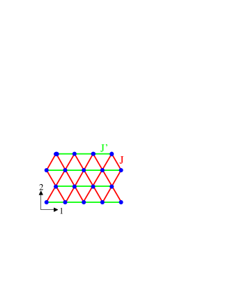
Figure 1: Triangular lattice on which the Heisenberg model (2.1) is defined.

Let us start with some specific model of a frustrated antiferromagnet on the triangular lattice shown in Fig.1. Exchange coupling in the horizontal bond is $J^{\prime}$ and the others are $J$. Quantum Hamiltonian ${\cal H}$ is given as

$${\cal H}=J\sum\vec{S}_{i}\cdot\vec{S}_{j}+J^{\prime}\sum\vec{S}_{i}\cdot\vec{S}_{j}+\cdots,$$ (2.1)

where $\vec{S}_{i}$ is $s={1\over 2}$ spin operator at site $i$, and the ellipsis denotes multi-spin and/or long-range interactions between spins, and the other notations are self-evident.

In the limit $J^{\prime}/J\ll 1$, the system reduces to the usual antiferromagnets on the square lattice and the ground state is expected to have the Néel order, whereas for $J^{\prime}/J\sim 1$, a new state is expected to appear. In order to study the system (2.1) by field-theory methods, we introduce the Schwinger boson operators $a_{i}=(a_{\uparrow i},a_{\downarrow i})$ at each site $i$, and then $\vec{S}_{i}$ is expressed as

$$\vec{S}_{i}={1\over 2}a^{\dagger}_{i}\vec{\sigma}a_{i},$$ (2.2)

where $\vec{\sigma}$ are the Pauli spin matrices. The following local constraint must be imposed as the physical-state condition in the Schwinger boson Hilbert space,

$$(a^{\dagger}_{\uparrow i}a_{\uparrow i}+a^{\dagger}_{\downarrow i}a_{\downarrow i})|\mbox{Phys}\rangle=|\mbox{Phys}\rangle.$$ (2.3)

We employ the path-integral methods to investigate the quantum system, and introduce CP¹ variables $z_{i}=(z_{\uparrow i},z_{\downarrow i})=(z_{1i},z_{2i})$ corresponding to $a_{i}$, which satisfy the constraint

$$\bar{z}_{\uparrow i}z_{\uparrow i}+\bar{z}_{\downarrow i}z_{\downarrow i}=1,$$ (2.4)

at each site $i$ and $\bar{z}_{\uparrow,\downarrow,i}$ is the complex conjugate of ${z}_{\uparrow,\downarrow,i}$. From the Hamiltonian (2.1), the partition function is given as

$$Z=\int[D\bar{z}Dz]_{{\rm CP}^{1}}\exp\Big{[}-\int d\tau\Big{(}\sum_{i}\bar{z}_{i}\cdot\dot{z}_{i}+{\cal H}(\bar{z},z)\Big{)}\Big{]},$$ (2.5)

where $\tau$ is the imaginary time, $\dot{z}_{i}={dz_{i}\over d\tau}$ and $\int[D\bar{z}Dz]_{{\rm CP}^{1}}$ denotes the integration over CP¹ variables $z_{i}$’s satisfying the constraint (2.4). ${\cal H}(\bar{z},z)$ is derived from (2.1) and (2.2). The above system is obviously invariant under a local gauge transformation $z_{i}(\tau)\rightarrow e^{i\theta_{i}(\tau)}z_{i}(\tau)$ with an arbitrary $\theta_{i}(\tau)$ satisfying $\theta_{i}(+\infty)=\theta_{i}(-\infty)$.

In the limit $J^{\prime}\rightarrow 0$, an effective field theory is obtained from the partition function $Z$ in (2.5) by integrating out the high-energy modes of $z_{i}$ (or $z_{i}$’s on all odd sitesCP-1 ; CP-2 ). The resultant theory is a CP¹ gauge model, which is described by the following action $S_{z}$ in the continuum spacetime with coordinate $x_{\mu}=(x_{0}=\tau,x_{1},x_{2})$,

$$S_{z}=\int d^{3}x\Big{[}{1\over g^{2}}\sum_{\mu}|D_{\mu}z|^{2}+{1\over e^{2}}\sum_{\mu<\nu}F_{\mu\nu}^{2}\Big{]},$$ (2.6)

where $D_{\mu}z=(\partial_{\mu}+iA_{\mu})z$, $F_{\mu\nu}=\partial_{\mu}A_{\nu}-\partial_{\nu}A_{\mu}$ with emergent gauge field $A_{\mu}$. In Eq.(2.6), $g,\;e$ are coupling constants. Bare value of $g$ is independent of the antiferromagnetic (AF) exchange coupling $J$, but it measures the solidity of the AF order, i.e., additional interactions that enhance (suppress) the AF order decrease (increase) the value of $g$. On the other hand, the bare value of $1/e$ is vanishing for the AF Heisenberg model with only the nearest-neighbor (NN) coupling but it acquire a finite value due to the renormalization effect of the high-energy modes. Multi-spin nonlocal interactions like a ring exchange coupling generate nonvanishing value of $1/e$Sawa . Varying the parameters $g$ and $e$ induces a phase transition and the structure of the ground state and low-energy excitations change drastically through the phase transition as we see in the following sections.

The field theory defined by (2.6) is obviously invariant under a U(1) gauge transformation. The continuum description (2.6) makes it unclear if this U(1) gauge symmetry is compact or noncompact one. As the original system of the AF magnets is defined on the lattice and transformation parameter $\theta_{i}(\tau)$ is defined mod $2\pi$, one may expect that the model (2.6) is a compact U(1) gauge system, in which topological nontrivial objects like instantons and vortices can exist. This expectation is qualitatively correct, but contribution from instanton configurations to the partition function is partly suppressed if there exists a Berry-phase term, $\int d^{3}x\epsilon_{\mu\nu\lambda}\partial_{\mu}F_{\nu\lambda}$ (where $\epsilon_{\mu\nu\lambda}$ is the antisymmetric tensor), in the action in addition to $S_{z}$Berry-1 ; Berry-2 ; Berry-3 . For the case $J^{\prime}\neq 0$, it is not easy to calculate the coefficient of the Berry phase, which plays a crucial role in the suppression of instantons. We shall not consider its effect in the following numerical investigation, and give comments on it in Sec.IVCS .

Phase structure of the CP^N-1 field theory has been studied by the $1/N$-expansion and numerical methodsCPN-1 ; CPN-2 ; CPN-3 . For the compact U(1) gauge case, a lattice-regularized version of (2.6) is quite useful for investigation on the CP¹ gauge model, and its action is given as follows,

$$A_{z} = {c_{1}\over 2}\sum_{x,\mu}\bar{z}_{x+\mu}U_{x,\mu}z_{x}+{c_{2}\over 2}\sum_{x,\mu<\nu}U_{x,\mu}U_{x+\mu,\nu}\bar{U}_{x+\nu,\mu}\bar{U}_{x,\nu}$$ (2.7)

$$+\mbox{c.c.},$$

where $x$ denotes site of the cubic lattice, and the coupling $c_{1}$ corresponds to $1/g^{2}$ and $c_{2}$ to $1/e^{2}$. Phase diagram has been obtained in the $c_{1}-c_{2}$ plane. See Fig.2. There are two phases separated by the critical line $c_{1}=c_{1c}(c_{2})$, one of which corresponds to the Néel state for $c_{1}>c_{1c}(c_{2})$ and the other state is a dimer state $c_{1}<c_{1c}(c_{2})$ in which the spinon $z_{x}$ is confined to a spin-triplet excitation $\bar{z}_{x}\vec{\sigma}z_{x}$. The phase transition across the transition line is of second order, and it belongs to the universality class of the $O(3)$ nonlinear sigma model in three dimensions ($3D$) (for small to medium values of $c_{2}$). The $s={1\over 2}$ AF Heisenberg model corresponds to $c_{1}>c_{1c}$, and the ground state has the AF long-range order. By introducing an inhomogeneity in the exchange coupling $J$ that enhances dimerization, the value of $c_{1}$ in the effective model (2.7) is decreased and the phase transition takes place from the Néel to dimer statesYoshi . Recently, numerical study on the inhomogeneous SU(2) AF Heisenberg model, which is essentially the same with that studied in Ref.Yoshi , was performed quite in detail and the existence of the phase transition from the Néel to dimer states was verifiedJanke1 . Phase transition belongs to the universality class of the $3D$ $O(3)$ nonlinear-sigma model, as predicted by the study of the effective lattice model (2.7).

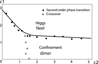
Figure 2: Phase diagram of the U(1) gauge theory of CP¹ spinonsCPN-2 . There are two phases.

As shown in Fig.2, the deconfined Coulomb phase does not exist in the model (2.7) of the U(1) gauge theory. Appearance of the Coulomb phase requires long-range and nonlocal interaction of gauge field $U_{x\mu}$, which may be generated by the coupling with gapless fermionsnonlocal ; nonlocal2 . In the pure quantum spin models without doping of holes, the deconfined phase is expected to appear by introducing frustrations because the Higgs mechanism is expected to take place by the appearance of the (short-range) spiral order. In that case, the U(1) gauge symmetry spontaneously breaks down to $Z_{2}$. It is known that the deconfined phase exists in the $3D$ $Z_{2}$ gauge models. There are interesting studies on spin liquids with deconfined spinons in the framework of the $Z_{2}$ gauge model. However, detailed and reliable study on the phase structure of the $Z_{2}$ gauge models relevant to the frustrated spin systems is still lacking. We study this problem in this paper.

Before going into details of the study on the frustrated AF magnets, let us comment on the validity of the present methods using the lattice field theory for studying AF magnets. To define quantum many-body systems without ambiguities, an ultra-violet (UV) regularization is necessary. In quantum spin models like (2.1), the spatial lattice naturally gives such an UV regularization. In the present approach, we first study the original model carefully and identify the relevant modes in the low-energy and low-momentum region. Through these observations, we obtain an effective field theory in the continuum spacetime. Then in order to study the effective field theory nonperturbatively (e.g. by means of the MC simulations), we reformulate it by using a spacetime lattice as a systematic regularization. Structure of the lattice model is deterimined by the symmetry of the effective field theory and we expect that details of the lattice model does not influence substantially physical results like phase structure and critical behaviors by the unversality-class argument. For the quantum SU(2) AF magnets, it is known that the results obtained by the effective CP¹ lattice model (2.7) are in good agreement with those obtained for the original AF Heisenberg model, as we explained above. Furthermore, phase structure of the lattice CP${}^{n}\;(n=1,\cdots,4)$ models obtained by the MC simulations is the same with that obtained by the $1/N$-expansion for the CP^N-1 field theory in the continuum spacetimeCPN-1 ; CPN-2 . These facts encourage us to apply the same methods to more complicated quantum spin systems like triangular AF spin systems with frustrations. More comments on the reliablity of the methods will be given in Sec.IV, after showing the main results of the present study in the following sections.

II.2 Effect of frustrations

The effect of the frustration in the AF magnets (2.1) can be studied in the framework of the CP¹ gauge field theory whose action has the following term $S_{\Lambda}$ in addition to $S_{z}$Sachdev1 ,

$$S_{\Lambda} = \int d^{3}x\sum_{\alpha=1,2}\Big{[}{1\over g^{2}_{\Lambda}}|D^{(2)}_{\mu}\Lambda_{\alpha}|^{2}+m_{\Lambda}|\Lambda_{\alpha}|^{2}+\lambda|\Lambda_{\alpha}|^{4}$$ (2.8)

$$+i\Lambda_{\alpha}\bar{z}\partial_{\alpha}\tilde{z}+\mbox{c.c.}\Big{]},$$

where $\Lambda_{\alpha}\;(\alpha=1,2)$ is a doubly-charged spatial vector field, $D^{(2)}_{\mu}=\partial_{\mu}+2iA_{\mu}$, and $\tilde{z}_{a}(x)=\epsilon_{ab}\bar{z}_{b}(x)$ ($\epsilon_{12}=-\epsilon_{21}=1,\;\epsilon_{11}=\epsilon_{22}=0$). Origin of the new term $S_{\Lambda}$ is as follows. The $J^{\prime}$-term in Eq.(2.1) generates terms like ${J^{\prime}\over J}\sum_{ij}|\bar{z}_{i}\cdot{\tilde{z}}_{j}|^{2}$ in the effective field theory, where the extra factor $1/J$ comes from the redefinition of the imaginary time $\tau\rightarrow\tau\times(aJ)$ ($a=$lattice spacing$=$often set unity). After inserting the following identity into the path-integral representation of the partition function,

$$\int d\Lambda_{ij}d\bar{\Lambda}_{ij}\;e^{-{J^{\prime}\over J}({J\over J^{\prime}}\Lambda_{ij}-iz_{i}\cdot\bar{\tilde{z}}_{j})({J\over J^{\prime}}\bar{\Lambda}_{ij}+i\bar{z}_{i}\cdot\tilde{z}_{j})}=\mbox{constant}$$ (2.9)

the above quartic term of $z_{i}$ is decoupled by a Hubbard-Stratonovich field $\Lambda_{\alpha}$. By the effects of renormalization of high-momentum modes, the extra terms in $S_{\Lambda}$ and renormalization of the mass, which preserve the local U(1) gauge symmetry, appear for describing low-energy behavior of the systemFNLambda .

Physical meaning of $S_{\Lambda}$ becomes transparent by considering the case $m_{\Lambda}<0$. In this case, we expect the nonvanishing expectation value of the field $\Lambda_{\alpha}$, i.e., $\langle\Lambda_{\alpha}\rangle\neq 0$. By solving the field equation derived from the action $S_{z}+S_{\Lambda}$, it is straightforward to verify that the low-energy configurations are given by,

$$z_{a}(x)={1\over\sqrt{2}}\Big{(}v_{a}(x)e^{ig^{2}\langle\vec{\Lambda}\rangle\cdot\vec{x}}+\epsilon_{ab}\bar{v}_{b}(x)e^{-ig^{2}\langle\vec{\Lambda}\rangle\cdot\vec{x}}\Big{)},$$ (2.10)

where $v_{a}(x)\;(a=1,2)$ is a slowly varying complex field satisfying $\sum_{a}|v_{a}(x)|^{2}=1$FNgauge ; FNU1 . For the configurations given by (2.10), the SU(2) spin field $\vec{S}(x)\equiv\bar{z}(x)\vec{\sigma}z(x)$ has the following form,

$$\vec{S}(x)=\vec{n}_{1}\cos(2g^{2}\langle\vec{\Lambda}\rangle\cdot\vec{x})+\vec{n}_{2}\sin(2g^{2}\langle\vec{\Lambda}\rangle\cdot\vec{x}),$$

$$\vec{n}_{1}={\rm Re}[\bar{\tilde{v}}\vec{\sigma}v],\;\;\vec{n}_{2}={\rm Im}[\bar{\tilde{v}}\vec{\sigma}v],$$

$$\vec{n}^{2}_{1}=\vec{n}^{2}_{2}=1,\;\;\vec{n}_{1}\cdot\vec{n}_{2}=0.$$ (2.11)

On the other hand, the “spin-nematic field” $\vec{n}_{3}=\vec{n}_{1}\times\vec{n}_{2}$ is given as $\vec{n}_{3}=\bar{v}\vec{\sigma}v$. It is obvious that $\vec{S}(x)$ in (2.11) corresponds to a spiral state if $\langle\vec{n}_{1}\rangle\neq 0,\;\langle\vec{n}_{2}\rangle\neq 0$.

By substituting Eq.(2.10) and $\Lambda_{0\alpha}=\langle\Lambda_{\alpha}\rangle$ into the continuum action $S_{z}+S_{\Lambda}$, low-energy effective theory is obtained. Condensation of $\Lambda_{\alpha}$ not only generates the spiral state of $\vec{S}$ but also a finite mass of the gauge field $A_{\mu}$. CP^N-1 model with a massive “gauge field” has been studied in the continuum spacetime by the $1/N$-expansion, but the obtained results are not reliable for the case of finite $N$ (in particular the case $N=2$) because an important effect at $O(1/N)$ coming from topological excitations is totally ignored theremassiveCPN . In fact, the condensation of $\Lambda_{\alpha}$ preserves the local $Z_{2}$ gauge invariance of the system because it carries double charge, and therefore the topological nontrivial excitation carrying a half-magnetic quantum, dubbed vison, exists as a low-energy excitationvison . Also in Ref.CSS , a quantum phase transition between a spin liquid with deconfined spinons and magnetically orderd state was studied, and various physical quantities were calculated by the $1/N$-expansion in an effective CP^N-1 field theory with a global U(1) symmetry. There it is assumed that effect of the vison can be ignored. Our study of the gauge model with the full $Z_{2}$ gauge symmetry in the present paper will show that this assumption is correct. See, for example, the calculation of the instanton density in Sec.III.

In the rest of the present paper, we shall study the effective $Z_{2}$ gauge theories obtained by substituting $\vec{\Lambda}=\langle\vec{\Lambda}\rangle$ and Eq.(2.10) into the action $S_{z}+S_{\Lambda}$. To this end, we reformulate it by using the lattice regularization that preserves the local $Z_{2}$ gauge symmetry. We use a cubic spacetime lattice because frustrations coming from AF coupling on the triangular lattice has disappeared by using the parameterization (2.10). The resultant lattice model is explicitly given by the following action,

$$A(c_{3}) = {c_{1}\over 2}\sum_{x,\mu}(\bar{v}_{x+\mu}U_{x,\mu}v_{x}+\bar{v}_{x}U_{x,\mu}v_{x+\mu})$$ (2.12)

$$+{c_{2}\over 2}\sum_{x,\mu<\nu}U_{x,\mu}U_{x+\mu,\nu}\bar{U}_{x+\nu,\mu}\bar{U}_{x,\nu}$$

$$+{c_{3}\over 2}\sum_{x,\mu}U^{2}_{x,\mu}+\mbox{c.c.},$$

where we explicitly show the dependence of the parameter $c_{3}$ in $A(c_{3})$, as we study the model with fixed values of $c_{3}$ in the following section. From the above consideration, $c_{3}\propto\langle\vec{\Lambda}\rangle^{2}$. Partition function of the gauge model (2.12) is given as

$$Z_{\rm Gauge}=\int[D\bar{z}Dz]_{{\rm CP}^{1}}[D\bar{U}DU]\;\exp A(c_{3}).$$ (2.13)

It is obvious that the system (2.12) has a local $Z_{2}$ gauge symmetry instead of the U(1) symmetry. Then we call $v_{x}$ $Z_{2}$CP¹ boson. In the limit $c_{3}\rightarrow\infty$, configurations of the gauge field are restricted to $U_{x,\mu}=\pm 1$ and the model reduces to a $Z_{2}$ gauge system. In the case $c_{3}\rightarrow\infty,\;c_{1}=0$, the system is the pure $Z_{2}$ gauge model in $3D$, which is dual to the $3D$ Ising model and has a second-order phase transition from the confined to deconfined “Coulomb” phases as $c_{2}$ is increased. This is in sharp contrast to the U(1) gauge model in $3D$, in which only the confined phase exists. As the deconfined phase corresponds to spin liquid with weakly interacting spinons, one may expect realization of a fractionalization phenomenon in frustrated AF magnets. In the following sections, we shall study phase structure of the model (2.12) by means of the MC simulations.

III Numerical studies

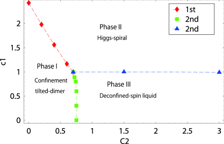
Figure 3: Phase diagram of the $Z_{2}$ gauge theory of CP¹ spinons. There are three phases.

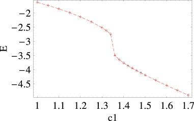
Figure 4: $E$ for $c_{2}=0.5$. There is sharp discontinuity at $c_{1}\simeq 1.35$ that indicates a first-order phase transition. System size is $L=24$.

III.1 $Z_{2}$ lattice gauge model of $Z_{2}$CP¹ spinon

We first study the $Z_{2}$ gauge model coupled with the field $v_{x}$ that corresponds to the limit $c_{3}\rightarrow\infty$ of the model (2.12). It is known that $Z_{2}$ gauge model coupled with single component Higgs boson describes nematic phase transition, and its phase structure was studied by both analytical and numerical methodsnematic . In these studies, importance of topological line defects (world lines of vison) was emphasized.

In order to investigate the phase structure of the $Z_{2}$ gauge model, we defined the model on the cubic lattice of size $L^{3}$ with the periodic boundary condition and calculated the “internal energy” $E=\langle A(\infty)\rangle/L^{3}$, the “specific heat” $C=\langle(A(\infty)-E)^{2}\rangle/L^{3}$, etc. We used the standard Metropolis algorithm for the MC simulationsMC . The typical statistics used was $10^{5}$ MC steps for each sample, and the averages and errors were estimated over $10\sim 20$ samples. Average acceptance probability was about $40\sim 50\%$.

The obtained phase diagram is shown in Fig.3. There are three phases, and calculation of various physical quantities gives the following identifications.

1. In the phase I, there is no AF long-range order and the gauge dynamics is realized in the confined phase. Low-energy excitations are spin-triplet bound states of the spinor $v_{x}$ (triplon), i.e., $\vec{n}_{1}(x),\;\vec{n}_{2}(x)$ in Eq.(2.11). We call this phase tilted dimer state.

2. In the phase II, there exists the magnetic long-range order of $v_{x}$, which corresponds to the spiral order of $\vec{S}(x)$, i.e., $\langle\vec{n}_{1}\rangle\neq 0,\;\langle\vec{n}_{2}\rangle\neq 0$. The gauge dynamics is in the Higgs phase because of the condensation of $v_{x}$. Low-energy excitations are gapless spin wave described by uncondensed component of $v_{x}$.

3. Phase III represents the paramagnetic spin liquid state. As for gauge dynamics, a deconfined “Coulomb phase” is realized, and the number of topological vortices is conserved. Low-energy excitations are massive spinon $v_{x}$.

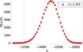
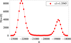
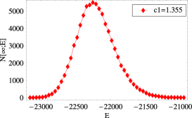
Figure 5: Distribution of $A(\infty)$ for $c_{2}=0.5$ and $c_{1}$ close to the phase transition point. The double-peak structure at $c_{1}=1.3545$ confirms the existence of the first-order phase transition. System size $L=24$.

We first show the numerical calculations of $E$ and $C$ for establishing the above phase diagram in Fig.3. We first focus on the transition from phase I to II. In Fig.4, we show calculation of $E$ as a function of $c_{1}$ with $c_{2}=0.5$. It is obvious that there exists a sharp discontinuity at $c_{1}\simeq 1.35$, which indicates a first-order phase transition. In order to verify it, we measured distribution of values of $A(\infty)$ generated in the MC steps, ${\cal N}[\infty;E]$, which is defined as

$$Z_{\rm Gauge} = \int dE\int[D\bar{z}Dz]_{{\rm CP}^{1}}[D\bar{U}DU]\;e^{A(\infty)}\delta(A(\infty)-E)$$ (3.14)

$$= \int dE\;{\cal N}[\infty;E].$$

We show the result near the critical point in Fig.5. At $c_{1}=1.3545$, ${\cal N}[\infty;E]$ has a double-peak structure, whereas the others have a single peak. From this result, we judge that the first-order phase transition takes place at $c_{1}=1.3545$.

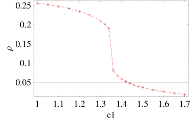
Figure 6: Instanton density for $c_{2}=0.5$ as a function of $c_{1}$. At the phase transition point $c_{1}\simeq 1.35$, it changes its behavior. System size $L=24$.

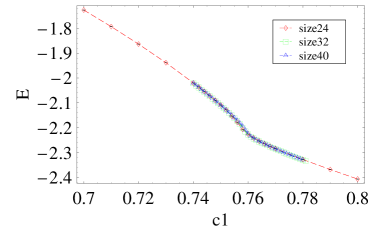
Figure 7: $E$ for $c_{1}=0.3$ as a function of $c_{2}$. System size $L=24,\;32,\;40$. There is almost no system-size dependence.

We also measured the instanton density $\rho(x)$ for $c_{2}=0.5$ as a function of $c_{1}$. $\rho(x)$ is defined as follows for the gauge field configuration $U_{x,\mu}=e^{i\theta_{x,\mu}},\;\theta_{x,\mu}=0,\;\pi$Inst-1 ; CPN-2 . First we consider the magnetic flux $\Theta_{x,\mu\nu}$ penetrating plaquette $(x,x+\mu,x+\mu+\nu,x+\nu)$

$$\Theta_{x,\mu\nu} = \theta_{x,\mu}+\theta_{x+\mu,\nu}-\theta_{x+\nu,\mu}-\theta_{x,\nu},$$ (3.15)

$$(-2\pi\leq\Theta_{x,\mu\nu}\leq 2\pi).$$

We decompose $\Theta_{x,\mu\nu}$ into its integer part $n_{x,\mu\nu}$, which represents the Dirac string (vortex line), and the remaining part $\tilde{\Theta}_{x,\mu\nu}$,

$$\Theta_{x,\mu\nu}=2\pi n_{x,\mu\nu}+\tilde{\Theta}_{x,\mu\nu},\;\;(-\pi\leq\tilde{\Theta}_{x,\mu\nu}\leq\pi).$$ (3.16)

Then instanton density $\rho(x)$ at the cube around the site $x+{\hat{0}\over 2}+{\hat{1}\over 2}+{\hat{2}\over 2}$ of the dual lattice is defined as

$$\begin{split}\rho(x)&=-{1\over 2}\sum_{\mu\nu\lambda}\epsilon_{\mu\nu\lambda}(n_{x+\mu,\nu\lambda}-n_{x,\nu\lambda})\\ &={1\over 4\pi}\sum_{\mu\nu\lambda}\epsilon_{\mu\nu\lambda}(\tilde{\Theta}_{x+\mu,\nu\lambda}-\tilde{\Theta}_{x,\nu\lambda}),\end{split}$$ (3.17)

where $\epsilon_{\mu\nu\lambda}$ is the antisymmetric tensor. From the above definition, it is obvious that $\rho\equiv\langle|\rho(x)|\rangle$ measures probability of creation/annihilation of magnetic vortex. In $3D$ $Z_{2}$ gauge theory, magnetic vortices in $3D$ can be regarded as world lines of flux quanta dubbed vison. Nonvanishing value of $\rho$ means that the number of visons is not conserved, and therefore condensation of the vison. The result of calculation of $\rho$ is shown in Fig.6. There is a sharp discontinuity at the phase transition $c_{1}\simeq 1.35$. In phase I, finite value of $\rho$ means large fluctuations of the gauge field and spinon $v_{x}$ is confined to gauge-invariant composites, $\vec{n}_{i}\;(i=1,2,3)$. This phenomenon is sometimes called dual Meissner effect. On the other hand in phase II, $\rho$ is strongly suppressed and the topological order exists. Later study on the spin correlation function reveals that this suppression is due to Higgs mechanism by the condensation of $v_{x}$.

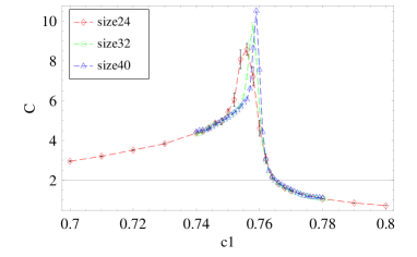
Figure 8: $C$ for $c_{1}=0.3$ as a function of $c_{2}$ with $L=24,\;32,\;40$. Its system-size dependence indicates that the phase transition is of second order. In addition to the standard MC simulations, we used multi-histogram methods to obtain reliable values of $C$ near the phase transition pointMHM .

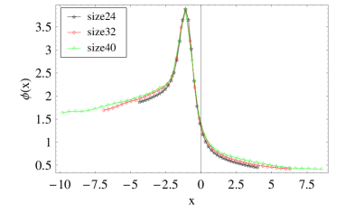
Figure 9: FSS for $c_{1}=0.3$. All data for $L=24,\;32,\;40$ can be fit by single function $\phi(x)$.

Next we consider the phase transition from phase I to III. We show $E$ and $C$ for $c_{1}=0.3$ in Figs.7 and 8. The results indicate that there exists a second-order phase transition at $c_{2}\simeq 0.76$. By the finite-size scaling (FSS) hypothesis for $C$,

$$C_{L}(\epsilon)=L^{\sigma/\nu}\phi(L^{1/\nu}\epsilon),$$ (3.18)

where $C_{L}$ is the “specific heat” of system size $L$, and $\epsilon\equiv(c_{2}-c_{2\infty})/c_{2\infty}$ with $c_{2\infty}$ (the critical coupling for $L\rightarrow\infty$), we estimated the critical exponents $\nu,\;\sigma$ by using the FSS (3.18) and obtained $\nu=0.63,\;\sigma=0.17$ and the critical coupling $c_{2\infty}=0.76$. The obtained scaling function $\phi(x)$ is shown in Fig.9. These values are very close to those of the pure $Z_{2}$ gauge model that are obtained from the data of the $3D$ Ising model by dualitydual .

We also measured instanton density $\rho$ and show the result in Fig.10. $\rho$ is a decreasing function of $c_{2}$ and changes its behavior at the phase transition point $c_{2}\simeq 0.76$.

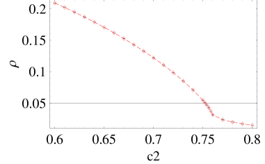
Figure 10: Instanton density for $c_{1}=0.3$ as a function of $c_{2}$. At the phase transition point $c_{2}\simeq 0.76$, it changes its behavior. System size $L=24$.

Finally, let us consider the phase transition from the phases II to III. Obtained $E$ has no system-size dependence. System-size dependence of $C$ is shown in Fig.11, from which we judge that the phase transition is of second order. By the FSS, the critical exponents are estimated as $\nu=0.65,\;\sigma=0.156,\;c_{2\infty}=0.93$. This value of $\nu$ should be compared with that of the $O(4)$ nonlinear sigma model in $3D$, $\nu_{O(4)}=0.75$. At present, it is not clear for us if the above two phase transitions belong to the same universality class.

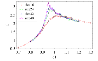
Figure 11: $C$ for $c_{2}=1.5$ as a function of $c_{1}$ with $L=16,\;24,\;32,\;40$. Its system-size dependence indicates that the phase transition is of second order.

In order to see (non)existence of the magnetic long-range order (LRO), we measured correlation functions of the spins $\vec{n}_{1}(x),\;\vec{n}_{2}(x)$ and $\vec{n}_{3}(x)$. They are defined as,

$$G_{i}(r)={1\over L^{3}}\sum_{x}\langle\vec{n}_{i}(x+r)\cdot\vec{n}_{i}(x)\rangle,\;\;\;i=1,2,3.$$ (3.19)

We exhibit the results in Figs.12, 13 and 14. It is obvious that only in phase II, they have the LRO. This LRO indicates a nonvanishing expectation value of $v_{x}$, $\langle v_{x}\rangle\neq 0$, in phase II. This understanding is supported by the measure of $\rho$, which shows that the gauge dynamics is in the Higgs phase in phase II.

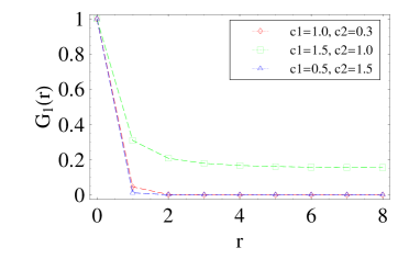
Figure 12: Correlation function of the spin field $\vec{n}_{1}(x)$. It has a long-range order only in phase II.

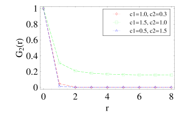
Figure 13: Correlation function of the spin field $\vec{n}_{2}(x)$. It has a long-range order only in phase II.

Figure 14: Correlation function of the spin-nematic field $\vec{n}_{3}(x)$. It has a long-range order only in phase II.

Figure 15: Spin gap as a function of $c_{1}$ for $c_{2}=1.5$.

We also calculated the spin gap as a function $c_{1}$ for $c_{2}=1.5$, i.e., from the spin liquid to spiral state. It is difficult to estimate the spin gap directly from the spin correlation functions $G_{i}(r)$. Then as in the previous studiesCPN-2 , we employ a Fourier transformation of the spin field, e.g., $\vec{n}_{3}(x)$,

$$\tilde{\vec{n}}_{3}(x_{0};p_{1},p_{2})=\sum_{x_{1},x_{2}}e^{ip_{1}x_{1}+ip_{2}x_{2}}\vec{n}_{3}(x).$$ (3.20)

In the continuum limit, the correlator of $\tilde{\vec{n}}_{3}(x_{0};p_{1},p_{2})$ behaves as

$$\langle\tilde{\vec{n}}_{3}(x_{0};p_{1},p_{2})\cdot\tilde{\vec{n}}_{3}(0;p_{1},p_{2})\rangle$$

$$\hskip 14.22636pt=\int\;dp_{0}{e^{ip_{0}x_{0}}\over\vec{p}^{2}+M^{2}_{s}}\propto e^{-\sqrt{p^{2}_{1}+p^{2}_{2}+M^{2}_{s}}x_{0}},$$ (3.21)

where $\vec{p}^{2}=\sum_{i=1,2,3}p^{2}_{i}$. In the practical calculation on the lattice, we put $p_{1}=p_{2}=2\pi/L$, and measured $\sqrt{p^{2}_{1}+p^{2}_{2}+M^{2}_{s}}$ from the correlation function of $\tilde{\vec{n}}_{3}(x_{0};p_{1},p_{2})$. We show the result $M_{s}$ as a function of $c_{1}$ in Fig.15. It is obvious that the spin gap $M_{s}$ is a continuous decreasing function of $c_{1}$ and is vanishing for $c_{1}>c_{1c}\simeq 1$. This result means that the spin excitation has a finite gap in the $Z_{2}$ spin liquid, whereas the spin wave in the spiral state is gapless.

From all the above calculations, we obtain the phase diagram shown in Fig.3.

III.2 U(1) gauge field coupled to $Z_{2}$CP¹ spinon: $c_{3}=0$ case

Let us consider the case $c_{3}=0$ of the system (2.12). The system with $c_{1}=0$ is nothing but the pure compact U(1) gauge model in $3D$. It is well-known that there is no phase transition and the system is always in the confined phase, though there is a crossover from dense-instanton to dilute-instanton regimes as the parameter $c_{2}$ is increased.

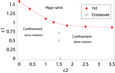
Figure 16: Phase diagram of the U(1) gauge theory of CP¹ spinons with $c_{3}=0$. There are two phases.

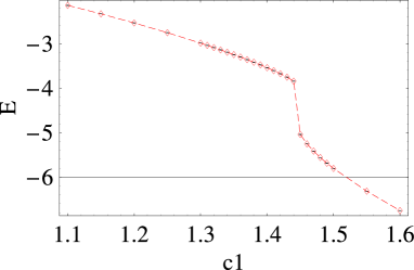
Figure 17: $E$ for $c_{2}=0.4$. There is sharp discontinuity at $c_{1}=1.44$ that indicates a first-order phase transition. System size is $L=24$.

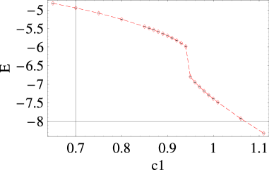
Figure 18: $E$ for $c_{2}=1.8$. There is sharp discontinuity at $c_{1}=0.95$ that indicates a first-order phase transition. System size is $L=24$.

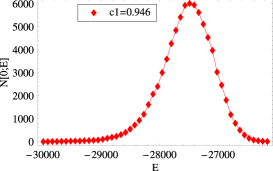
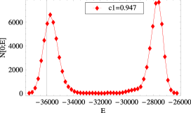
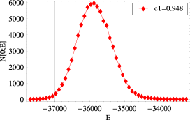
Figure 19: Distribution of $A(0)$ for $c_{2}=1.8$ and $c_{1}$ close to the phase transition point. The double-peak structure at $c_{1}=0.947$ confirms the existence of the first-order phase transition. System size $L=24$.

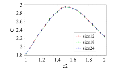
Figure 20: $C$ for $c_{1}=0.5$. System size $L=12,\;18,\;24$. There is no system-size dependence, i.e., the second-order phase transition in the $Z_{2}$ gauge model reduces to a crossover. The deconfined spin-liquid phase does not exists in the model with $c_{3}=0$.

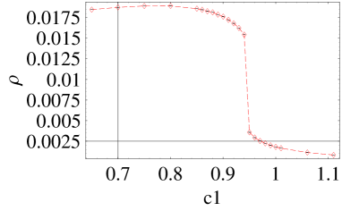
Figure 21: Instanton density for $c_{2}=1.8$ as a function of $c_{1}$. At the phase transition point $c_{1}\simeq 0.95$, there is a sharp discontinuity. System size $L=24$.

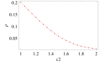
Figure 22: Instanton density for $c_{1}=0.5$ as a function of $c_{2}$. There is no anomalous behavior at the crossover $c_{2}\simeq 1.5$. System size $L=24$.

We show the obtained phase diagram of the system (2.12) with $c_{3}=0$ in Fig.16. There are two phases, (i) phase I is the dimer phase with confinement of spinons and without any long-range order, (ii) phase II is the spiral state with the condensation of $v_{x}$. Phase transitions separating these two phases are of first order as the calculations of $E$ in Figs.17 and 18 indicates. In order to verify this observation, we measured the distribution of $A(0)$, ${\cal N}[0;E]$, in the MC steps. From Fig.19, it is obvious that on the critical line ${\cal N}[0;E]$ has a double-peak structure whereas it does not off the critical line.

The second-order phase transition that exists in the $Z_{2}$ gauge model of spinons from the confined to deconfined phases disappears in the system with $c_{3}=0$. There is a crossover line emanating from the crossover point of the pure compact U(1) gauge model in $3D$. See Fig.20. This fact strongly influences structure of the ground state and low-energy excitations of the original spin system. Absence of the deconfined phase means that the spin liquid phase does not exist in the present case. We measured the instanton density$\rho$ to verify the above conclusion. In particular in the dilute-instanton regime $c_{2}>1.5$, the instanton density $\rho$ is small even in the confined phase $c_{1}<c_{1c}(c_{2})$, but it decreases rapidly at the phase transition $c_{1}=c_{1c}(c_{2})$ to the Higgs phase. See Fig.21. On the other hand for $c_{1}=0.5$, $\rho$ is a decreasing function of $c_{2}$ but does not exhibit any anomalous behavior at the crossover $c_{2}\simeq 1.5$. See Fig.22.

We calculated the spin correlation functions in each phase and verified that the spin LRO exists only in the Higgs phase $c_{1}>c_{1c}$.

III.3 Massive U(1) gauge field coupled with $Z_{2}$CP¹ spinon: $c_{3}=1.0$ case

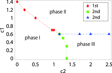
Figure 23: Phase diagram of the U(1) gauge theory of CP¹ spinons with $c_{3}=1.0$. There are three phases as in the $Z_{2}$ gauge model.

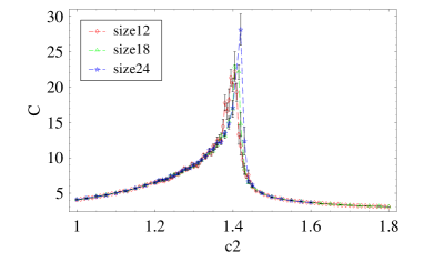
Figure 24: $C$ for $c_{1}=0.3$. System size $L=12,\;18,\;24$.

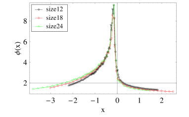
Figure 25: FSS for $c_{1}=0.3$. All data for $L=12,\;18,\;24$ can be fit by single function $\phi(x)$.

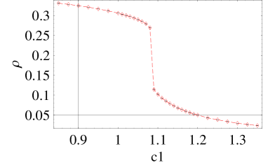
Figure 26: Instanton density for $c_{2}=0.5$ as a function of $c_{1}$. At $c_{1}\simeq 1.1$, there is sharp discontinuity corresponding to the first-order phase transition. System size $L=24$.

Figure 27: Instanton density for $c_{1}=0.3$ as a function of $c_{2}$. At $c_{2}\simeq 1.4$, $\rho$ changes its behavior. System size $L=24$.

Finally let us consider the case $c_{3}=1.0$. We also investigated the case $c_{3}=2.0$ and obtained similar results. In the present case $c_{3}>0$, the gauge field $U_{x,\mu}$ is a $U(1)$ variable, but local U(1) gauge symmetry is explicitly broken down to $Z_{2}$ by both the hopping term of $v_{x}$ and the mass term of the gauge field, i.e., $U_{x,\mu}^{2}+\mbox{c.c.}$ It is expected that the mass term of the gauge field is a relevant perturbation and therefore the phase structure of the system $c_{3}>0$ is qualitatively the same with that of the $Z_{2}$ gauge theory studied in Sec.III.A.

We show the obtained phase diagram in Fig.23. There are three phases similarly to the $Z_{2}$ gauge theory of spinons, as it is expected. In Figs.24 and 25, we show $C$ as a function of $c_{2}$ for $c_{1}=0.3$ and the FSS scaling function obtained from these data. Critical exponents are estimated as $\nu=1.26,\;\sigma=0.43$ and $c_{2\infty}=1.44$. From the above result, we think that the present phase transition does not belong to the universality class of the $3D$ Ising model. At phase transitions from the tilted-dimer to spiral phases, $E$, the distribution of ${\cal N}[1;E]$ and the instanton density $\rho$ have similar behaviors to those in the previous cases of the first-order phase transition. In Figs.26 and 27, we show the result of the instanton density.

IV Conclusion and discussion

In the present paper, we derived effective gauge models that describe low-energy properties of antiferromagnets with frustrations in $2D$, and studied their phase structure mostly by means of MC simulations. We found that generally there are three phases in the models, (i) phase of the tilted dimer state with spin-triplet excitations, (ii) the spiral state with gapless spin wave, (iii) the spin liquid with weakly interacting spinons. We identified the order of the phase transitions and estimated values of the critical exponents of the second-order phase transitions. The investigation suggests that for the spin liquid to appear, multi-spin and nonlocal interactions are necessary in the original spin systems.

In order to verify the validity of the above results, it is important and also possible to study spin systems on layered $3D$ triangular lattice at finite temperature ($T$) by means of the Schwinger boson (CP¹) representations. In this case, the systems can be studied directly with the spatial lattice as a regularization. In the path-integral representation of the partition function $Z$ in (2.5) at finite $T$, the $\tau$-dependence of $z_{i}$ is ignored. Then the path-integral over CP¹ variables $z_{i}$’s in $Z$ can be performed without any difficulties by the MC simulations. At present we are studying these systems, and have obtained preliminary results that support the conclusion in the present paperNKIM .

In the present paper, we mostly focus on the (short-range) spiral state with $\langle\Lambda_{ij}\rangle\propto\langle z_{i}\cdot\bar{\tilde{z}}_{j}\rangle=\Lambda_{0}\neq 0$. There is another possibility of canted state like $\langle\Lambda_{i,i+\hat{1}}\rangle=(-)^{i}\Lambda_{0}\neq 0$. This state can be regarded as a state with a ferromagnetic order in the AF background. This state also breaks the U(1) gauge invariance down to the $Z_{2}$ as the (short-range) spiral state does, and therefore results obtained in the present paper are expected to be applicable to the canted state.

Finally let us comment on effects of the Berry phase. As we explained in Sec.II, the Berry phase appears after integrating out the high-energy modes in the path integral in order to derive the effective field theory of AF magnets. The Berry phase may play an important role though qualitative phase structure is not changed by its existenceFNBerry1 . Whether the suppression of the instantons occurs by the Berry phase strongly depends on its coefficient. For example in the inhomogeneous AF Heisenberg model on a square lattice, the coefficient depends on the magnitude of the inhomogeneity and is generally an irrationalYoshi . Suppression of instantons does not occur in that case and the Néel-dimer phase transition belongs to the universality class of the classical $3D\;O(3)$ nonlinear sigma model, which is equivalent to the CP¹ gauge model (2.6) without the Berry phase. This result was verified by the numerical study of the inhomogeneous SU(2) AF Heisenberg model. We expect that nonvanishing frustration coupling $J^{\prime}$ gives a similar effect on the Berry phase’s coefficient because the most dominant NN spin pair configuration is shifted from $z_{ia}=\epsilon_{ab}\bar{z}_{jb}$ ($i,j=$ site, $a,b=$ spinor indices) on path-integrating out high-energy modes. If this is the case, the Berry phase gives only negligible effects on critical behavior of the systems under study, and the FSS used in the present paper gives reliable estimation of the critical exponentsFNBerry2 .