SpicyMKL

Abstract

We propose a new optimization algorithm for Multiple Kernel Learning (MKL) called SpicyMKL, which is applicable to general convex loss functions and general types of regularization. The proposed SpicyMKL iteratively solves smooth minimization problems. Thus, there is no need of solving SVM, LP, or QP internally. SpicyMKL can be viewed as a proximal minimization method and converges super-linearly. The cost of inner minimization is roughly proportional to the number of active kernels. Therefore, when we aim for a sparse kernel combination, our algorithm scales well against increasing number of kernels. Moreover, we give a general block-norm formulation of MKL that includes non-sparse regularizations, such as elastic-net and $\ell_{p}$ -norm regularizations. Extending SpicyMKL, we propose an efficient optimization method for the general regularization framework. Experimental results show that our algorithm is faster than existing methods especially when the number of kernels is large ($>$ 1000).

1 Introduction

Kernel methods are powerful nonparametric methods in machine learning and data analysis. Typically a kernel method fits a decision function that lies in some Reproducing Kernel Hilbert Space (RKHS) (Aronszajn, 1950; Schölkopf and Smola, 2002). In such a learning framework, the choice of a kernel function can strongly influence the performance. Instead of using a fixed kernel, Multiple Kernel Learning (MKL) (Lanckriet et al., 2004; Bach et al., 2004; Micchelli and Pontil, 2005) aims to find an optimal combination of multiple candidate kernels.

More specifically, we assume that a data point $x\in{\mathcal{X}}$ lies in a space $\mathcal{X}$ and we are given $M$ candidate kernel functions $k_{m}:{\mathcal{X}}\times{\mathcal{X}}\rightarrow{\mathbb{R}}$ ($m=1,\ldots,M$). Each kernel function corresponds to one data source. A conical combination of $k_{m}$ ($m=1,\ldots,M$) gives the combined kernel function $\bar{k}=\sum_{m=1}^{M}d_{m}k_{m}$, where $d_{m}$ is a nonnegative weight. Our goal is to find a good set of kernel weights based on some training examples.

While the MKL framework has opened up a possibility to combine multiple heterogeneous data sources (numerical features, texts, links) in a principled manner, it is also posing an optimization challenge: the number of kernels can be very large. Instead of arguing whether polynomial kernel or Gaussian kernel fits a given problem better, we can simply put both of them into an MKL algorithm; instead of evaluating which band-width parameter to choose, we can simply generate kernels from all the possible combinations of parameter values and feed them to an MKL algorithm. See Gehler and Nowozin (2009); Tomioka and Suzuki (2009).

Various optimization algorithms have been proposed in the context of MKL. In the pioneering work of Lanckriet et al. (2004), MKL was formulated as a semi-definite programming (SDP) problem. Bach et al. (2004) showed that the SDP can be reduced to a second order conic programming (SOCP) problem. However solving SDP or SOCP via general convex optimization solver can be quite heavy especially for large number of samples.

More recently, wrapper methods have been proposed. A wrapper method iteratively solves a single kernel learning problem (e.g., SVM), for a given kernel combination and then updates the kernel weights. A nice property of this type of methods is that it can make use of existing well-tuned solvers for SVM. Semi-Infinite Linear Program (SILP) approach proposed by Sonnenburg et al. (2006) utilizes a cutting plane method for the update of the kernel weights. SILP often suffers from instability of the solution sequence especially when the number of kernels is large, i.e. the intermediate solution oscillates around the optimal one (Rakotomamonjy et al., 2008). SimpleMKL proposed by Rakotomamonjy et al. (2008) performs a reduced gradient descent on the kernel weights. Simple MKL resolves the drawback of SILP, but still it is a first order method. Xu et al. (2009) proposed a novel Level Method (which we call LevelMKL) as an improvement of SILP and SimpleMKL. LevelMKL is rather efficient than SimpleMKL and scales well against the number of kernels by utilizing sparsity but it shows unstable behavior as the algorithm proceeds because LevelMKL solves Linear Programming (LP) and Quadratic Programming (QP) of increasingly large size as its iteration proceeds. HessianMKL proposed by Chapelle and Rakotomamonjy (2008) replaced the gradient descent update of SimpleMKL with a Newton update. At each iteration, HessianMKL solves a QP problem with the size of the number of kernels to obtain the Newton update direction. HessianMKL shows second order convergence, but scales badly against the number of kernels because the size of the QP grows as the number of kernels grows.

The first contribution of this article is an efficient optimization algorithm for MKL based on the block 1-norm formulation introduced in Bach et al. (2005) (see also Bach et al. (2004)); see Eq. (4). The block 1-norm formulation can be viewed as a kernelized version of group lasso (Yuan and Lin, 2006; Bach, 2008). For group lasso, or more generally sparse estimation, efficient optimization algorithms have recently been studied intensively, boosted by the development of compressive sensing theory (Candes et al., 2006). Based on this view, we extend the dual augmented-Lagrangian (DAL) algorithm (Tomioka and Sugiyama, 2009) recently proposed in the context of sparse estimation to kernel-based learning. DAL is efficient when the number of unknown variables is much larger than the number of samples. This enables us to scale the proposed algorithm, which we call SpicyMKL, to thousands of kernels.

Compared to the original DAL algorithm (Tomioka and Sugiyama, 2009), our presentation is based on an application of proximal minimization framework (Rockafellar, 1976) to the primal MKL problem. We believe that the current formulation is more transparent compared to the dual based formulation in Tomioka and Sugiyama (2009), because we are not necessarily interested in solving the dual problem. Moreover, we present a theorem on the rate of convergence.

SpicyMKL does not need to solve SVM, LP or QP internally as previous approaches. Instead, it minimizes a smooth function at every step. The cost of inner minimization is proportional to the number of active kernels. Therefore, when we aim for a sparse kernel combination, the proposed algorithm is efficient even when thousands of candidate kernels are used. In fact, we show numerically that we are able to train a classifier with 3000 kernels in less than 10 seconds.

Learning combination of kernels, however, has recently recognized as a more complex task than initially thought. Cortes (2009) pointed out that learning convex kernel combination with an $\ell_{1}$-constraint on the kernel weights (see Section 2) produces an overly sparse (many kernel weights are zero) solution, and it is often outperformed by a simple uniform combination of kernels; accordingly they proposed to use an $\ell_{2}$-constraint instead (Cortes et al., 2009). In order to search for the best trade-off between the sparse $\ell_{1}$-MKL and the uniform weight combination, Kloft et al. (2009) proposed a general $\ell_{p}$-norm constraint and Tomioka and Suzuki (2009) proposed an elastic-net regularization, both of which smoothly connect the 1-norm MKL and uniform weight combination.

The second contribution of this paper is to extend the block-norm formulation that allows us to view these generalized MKL models in a unified way, and provide an efficient optimization algorithm. We note that while this paper was under review, Kloft et al. (2010) presented a slightly different approach that results in a similar optimization algorithm. However, our formulation provides clearer relationship between the block-norm formulation and kernel-combination weights and is more general.

This article is organized as follows. In Section 2, we introduce the framework of block 1-norm MKL through Tikhonov regularization on the kernel weights. In Section 3, we propose an extension of DAL algorithm to kernel-learning setting. Our formulation of DAL algorithm is based on a primal application of the proximal minimization framework (Rockafellar, 1976), which also sheds a new light on DAL algorithm itself. Furthermore, we discuss how we can carry out the inner minimization efficiently exploiting the sparsity of the 1-norm MKL. In Section 4, we extend our framework to general class of regularizers including the $\ell_{p}$-norm MKL (Kloft et al., 2009) and Elastic-net MKL (Tomioka and Suzuki, 2009). We extend the proposed SpicyMKL algorithm for the generalized formulation and also present a simple one-step optimization procedure for some special cases that include Elastic-net MKL and $\ell_{p}$-norm MKL. In Section 5, we discuss the relations between the existing methods and the proposed method. In Section 6, we show the results of numerical experiments. The experiments show that SpicyMKL is efficient for block 1-norm regularization especially when the number of kernels is large. Moreover the one-step optimization procedure for elastic-net regularization shows quite fast convergence. In fact, it is faster than those methods with block 1-norm regularization. Finally, we summarize our contribution in Section 7. The proof of super-linear convergence of the proposed SpicyMKL is given in Appendix A.

A Matlab^\tiny{R}⃝ implementation of SpicyMKL is available at the following URL:

http://www.simplex.t.u-tokyo.ac.jp/~s-taiji/software/SpicyMKL

2 Framework of MKL

In this section, we first consider a learning problem with fixed kernel weights in Section 2.1. Next in Section 2.2, using Tikhonov regularization on the kernel weights, we derive a block 1-norm formulation of MKL, which can be considered as a direct extension of group lasso in the kernel-based learning setting. In addition, we discuss the connection between the current block 1-norm formulation and the squared block 1-norm formulation. In Section 2.3, we present a finite dimensional version of the proposed formulation and prepare notations for the later sections.

2.1 Fixed kernel combination

We assume that we are given $N$ samples $(x_{i},y_{i})_{i=1}^{N}$ where $x_{i}$ belongs to an input space ${\mathcal{X}}$ and $y_{i}$ belongs to an output space ${\mathcal{Y}}$ (usual settings are ${\mathcal{Y}}=\{\pm 1\}$ for classification and ${\mathcal{Y}}={\mathbb{R}}$ for regression). We define the Gram matrix with respect to the kernel function $k_{m}$ as $K_{m}=(k_{m}(x_{i},x_{j}))_{i,j}$. We assume that the Gram matrix $K_{m}$ is positive definite.

We first consider a learning problem with fixed kernel weights. More specifically, we fix non-negative kernel weights $d_{1},d_{2},\ldots,d_{M}$ and consider the RKHS $\bar{{\mathcal{H}}}$ corresponding to the combined kernel function $\bar{k}=\sum_{m=1}^{M}d_{m}k_{m}$. The (squared) RKHS norm of a function $\bar{f}$ in $\bar{{\mathcal{H}}}$ is written as follows (see Sec 6 in Aronszajn (1950), and also Micchelli and Pontil (2005)):

$$\|\bar{f}\|_{\bar{{\mathcal{H}}}}^{2}:=\min_{f_{1}\in{\mathcal{H}}_{1},\ldots,f_{M}\in{\mathcal{H}}_{M}}\sum_{m=1}^{M}\frac{\|f_{m}\|_{{\mathcal{H}}_{m}}^{2}}{d_{m}}\quad{\rm s.t.}\quad\bar{f}=\sum_{m=1}^{M}f_{m},$$ (1)

where ${\mathcal{H}}_{m}$ is the RKHS that corresponds to the kernel function $k_{m}$. Accordingly, with a fixed kernel combination, a supervised learning problem can be written as follows:

$$\mathop{\mathrm{minimize}}_{f_{1}\in{\mathcal{H}}_{1},\ldots,f_{M}\in{\mathcal{H}}_{M},b\in{\mathbb{R}}} \sum_{i=1}^{N}\ell\left(y_{i},\textstyle\sum_{m=1}^{M}f_{m}(x_{i})+b\right)+\frac{C}{2}\sum_{m=1}^{M}\frac{\|f_{m}\|_{{\mathcal{H}}_{m}}^{2}}{d_{m}},$$ (2)

where $b$ is a bias term and $\ell(y,f)$ is a loss function, which can be the hinge loss $\max(1-yf,0)$ or the logistic loss $\log(1+\exp(-yf))$ for a classification problem, or the squared loss $(y-f)^{2}$ or the SVR loss $\max(|y-f|-\epsilon,0)$ for a regression problem. The above formulation may not be so useful in practice, because we can compute the combined kernel function $\bar{k}$ and optimize over $\bar{f}$ instead of optimizing $M$ functions $f_{1},\ldots,f_{M}$. However, explicitly handling the kernel weights allows us to consider various generalizations of MKL in a unified manner.

2.2 Learning kernel weights

In order to learn the kernel weights $d_{m}$ through the objective (2), there is clearly a need for regularization, because the objective is a decreasing function of the kernel weights $d_{m}$. Roughly speaking, the kernel weight $d_{m}$ corresponds to the complexity allowed for the $m$th classifier component $f_{m}$, without regularization, we can get a serious over-fitting.

One way to prevent such overfitting is to penalize the increase of the kernel weight $d_{m}$ by adding a penalty term. Adding a linear penalty term, we have the following optimization problem.

$$\mathop{\mathrm{minimize}}_{\begin{subarray}{c}f_{1}\in{\mathcal{H}}_{1},\ldots,f_{M}\in{\mathcal{H}}_{M},\\ b\in{\mathbb{R}},\\ d_{1}\geq 0,\ldots,d_{M}\geq 0\end{subarray}} \sum_{i=1}^{N}\ell\left(y_{i},\textstyle\sum_{m=1}^{M}f_{m}(x_{i})+b\right)+\frac{C}{2}\sum_{m=1}^{M}\left(\frac{\|f_{m}\|_{{\mathcal{H}}_{m}}^{2}}{d_{m}}+d_{m}\right).$$ (3)

The above formulation reduces to the block 1-norm introduced in Bach et al. (2005) by explicitly minimizing over $d_{m}$ as follows:

$$\mathop{\mathrm{minimize}}_{\begin{subarray}{c}f_{1}\in{\mathcal{H}}_{1},\ldots,f_{M}\in{\mathcal{H}}_{M},\\ b\in{\mathbb{R}}\end{subarray}} \sum_{i=1}^{N}\ell\left(y_{i},\textstyle\sum_{m=1}^{M}f_{m}(x_{i})+b\right)+C\sum_{m=1}^{M}\|f_{m}\|_{{\mathcal{H}}_{m}},$$ (4)

where we used the inequality of arithmetic and geometric means; the minimum with respect to $d_{m}$ is obtained by taking $d_{m}=\|f_{m}\|_{{\mathcal{H}}_{m}}$.

The regularization term in the above block 1-norm formulation is the linear sum of RKHS norms. This formulation can be seen as a direct generalization of group lasso (Yuan and Lin, 2006) to the kernel-based learning setting, and motivates us to extend an efficient algorithm for sparse estimation to MKL.

The block 1-norm formulation (4) is related to the following squared block 1-norm formulation considered in Bach et al. (2004); Sonnenburg et al. (2006); Zien and Ong (2007); Rakotomamonjy et al. (2008):

$$\mathop{\mathrm{minimize}}_{f_{1}\in{\mathcal{H}}_{1},\ldots,f_{M}\in{\mathcal{H}}_{M},b\in{\mathbb{R}}} \sum_{i=1}^{N}\ell\left(y_{i},\textstyle\sum_{m=1}^{M}f_{m}(x_{i})+b\right)+\frac{\tilde{C}}{2}\left(\sum_{m=1}^{M}\|f_{m}\|_{{\mathcal{H}}_{m}}\right)^{2},$$ (5)

which is obtained by considering a simplex constraint on the kernel weights (Kloft et al., 2009) instead of penalizing them as in (3).

The solution of the two problems (4) and (5) can be mapped to each other. In fact, let $\{f_{m}^{\star}\}_{m=1}^{M}$ be the minimizer of the block 1-norm formulation (4) with the regularization parameter $C$ and let $\tilde{C}$ be

$$\textstyle\tilde{C}=C(\sum_{m=1}^{M}\|f_{m}^{\star}\|_{{\mathcal{H}}_{m}}).$$ (6)

Then $\{f_{m}^{\star}\}$ also minimizes the squared block 1-norm formulation (5) with the regularization parameter $\tilde{C}$ because of the relation

$$\partial_{f_{m}}\frac{1}{2}\left(\sum_{m=1}^{M}\|f_{m}\|_{{\mathcal{H}}_{m}}\right)^{2}=\left(\sum_{m=1}^{M}\|f_{m}\|_{{\mathcal{H}}_{m}}\right)\partial_{f_{m}}\|f_{m}\|_{{\mathcal{H}}_{m}},$$

where $\partial_{f_{m}}$ is a subdifferential with respect to $f_{m}$.

2.3 Representer theorem

In this subsection, we convert the block 1-norm MKL formulation (4) into a finite dimensional optimization problem via the representer theorem and prepare notation for later sections.

The optimal solution of (4) is attained in the form of $f_{m}(x)=\sum_{i=1}^{N}k_{m}(x,x_{i})\alpha_{m,i}$ due to the representer theorem (Kimeldorf and Wahba, 1971). Thus, the optimization problem (4) is reduced to the following finite dimensional optimization problem:

$$\mathop{\mathrm{minimize}}\limits_{\alpha\in{\mathbb{R}}^{NM},b\in{\mathbb{R}}}\quad\sum\limits_{i=1}^{N}\ell(y_{i},\textstyle\sum_{m=1}^{M}\sum_{j=1}^{N}k_{m}(x_{i},x_{j})\alpha_{m,j}+b)+C\sum\limits_{m=1}^{M}\|\alpha_{m}\|_{K_{m}}$$

where $\alpha_{m}=(\alpha_{m,1},\dots,\alpha_{m,N})^{\top}$, $\alpha=(\alpha_{1}^{\top},\dots,\alpha_{M}^{\top})^{\top}\in{\mathbb{R}}^{NM}$, and the norm $\|\cdot\|_{K_{m}}$ is defined through the inner product $\langle\alpha_{m},\beta_{m}\rangle_{K_{m}}:=\alpha_{m}^{\top}K_{m}\beta_{m}$ for $\alpha_{m},\beta_{m}\in{\mathbb{R}}^{N}$. We also define the norm $\|\cdot\|_{\bar{K}}$ through the inner product $\langle\alpha,\beta\rangle_{\bar{K}}:=\sum_{m=1}^{M}\langle\alpha_{m},\beta_{m}\rangle_{K_{m}}$ for $\alpha,\beta\in{\mathbb{R}}^{NM}$.

For simplicity we rewrite the above problem as

$$\mathop{\mathrm{minimize}}_{\alpha\in{\mathbb{R}}^{NM},b\in{\mathbb{R}}}\quad\underbrace{L(\bar{K}\alpha+b\mathbf{1})+\phi_{C}(\alpha)}_{=:L_{C}(\alpha,b)},$$ (7)

where $\bar{K}=(K_{1},\dots,K_{M})\in{\mathbb{R}}^{N\times NM}$, $\mathbf{1}=(1,\dots,1)^{\top}$ and

$$L(z)=\sum_{i=1}^{N}\ell(y_{i},z_{i}),~{}~{}~{}~{}~{}$$

$$\phi_{C}(\alpha)=\sum\limits_{m=1}^{M}\phi_{C}^{(m)}(\alpha_{m})=C\sum\limits_{m=1}^{M}\|\alpha_{m}\|_{K_{m}}.$$

3 A dual augmented-Lagrangian method for MKL

In this section, we first present an extension of dual augmented-Lagrangian (DAL) algorithm to kernel-learning problem through a new approach based on the proximal minimization framework (Rockafellar, 1976). Second, assuming that the loss function is twice differentiable, we discuss how we can compute each minimization step efficiently in Section 3.3. Finally, the method is extended to the situation where the loss function is not differentiable in Section 3.4.

3.1 MKL optimization via proximal minimization

Starting from some initial solution $(\alpha^{(1)},b^{(1)})$, the proximal minimization algorithm (Rockafellar, 1976) iteratively minimizes the objective (7) together with proximity terms as follows:

$$(\alpha^{(t+1)}\!,b^{(t+1)})\!=\!\!\!\!\mathop{\mathrm{argmin}}_{\alpha\in{\mathbb{R}}^{MN},b\in{\mathbb{R}}}\!\!\Biggl{(}L_{C}(\alpha,b)+\!\!\frac{1}{2\gamma^{(t)}}\Bigl{(}\|\alpha-\alpha^{(t)}\|_{\bar{K}}^{2}+(b-b^{(t)})^{2}\Bigr{)}\Biggr{)},$$ (8)

where $0<\gamma^{(1)}\leq\gamma^{(2)}\leq\gamma^{(3)}\leq\ldots$ is a nondecreasing sequence of proximity parameters and $(\alpha^{(t)},b^{(t)})$ is an approximate minimizer at the $t$th iteration; $L_{C}$ is the (regularized) objective function (7). The last two terms in the right-hand side are proximity terms that tries to keep the next solution $(\alpha^{(t+1)},b^{(t+1)})$ close to the current solution $(\alpha^{(t)},b^{(t)})$. Thus, we call the minimization problem (8) a proximal MKL problem. Solving the proximal MKL problem (8) seems as difficult as solving the original MKL problem in the primal. However, when we consider the dual problems, solving the dual of proximal MKL problem (8) is a smooth minimization problem and can be minimized efficiently, whereas solving the dual of the original MKL problem (7) is a non-smooth minimization problem and not necessarily easier than solving the primal.

The update equation can be interpreted as an implicit gradient method on the objective function $L_{C}(\alpha,b)$. In fact, by taking the subgradient of the update equation (8) and equating it to zero, we have

$$\alpha_{m}^{(t+1)} \in\alpha_{m}^{(t)}-\gamma^{(t)}K_{m}^{-1}\partial_{\alpha_{m}}L_{C}(\alpha^{(t+1)},b^{(t+1)}),$$

$$b^{(t+1)} \in b^{(t)}-\gamma^{(t)}\partial_{b}L_{C}(\alpha^{(t+1)},b^{(t+1)}).$$

This implies the $t$th update step is a subgradient of the original objective function $L_{C}$ at the next solution $(\alpha_{m}^{(t+1)},b^{(t+1)})$.

The super-linear convergence of proximal minimization algorithm (Rockafellar, 1976; Bertsekas, 1982; Tomioka et al., 2011) can also be extended to kernel-based learning setting as in the following theorem.

Theorem 1.

Suppose the problem (7) has a unique optimal solution $\alpha^{\ast}$, $b^{\ast}$, and there exist a scalar $\sigma>0$ and a $\delta$-neighborhood ($\delta>0$) of the optimal solution such that

$$L_{C}(\alpha,b)\geq L_{C}(\alpha^{\ast},b^{\ast})+\sigma(\|\alpha-\alpha^{\ast}\|_{\bar{K}}^{2}+(b-b^{\ast})^{2}),$$ (9)

for all $(\alpha,b)\in{\mathbb{R}}^{MN}\times{\mathbb{R}}$ satisfying $\|\alpha-\alpha^{\ast}\|_{\bar{K}}^{2}+(b-b^{\ast})^{2}\leq\delta^{2}$. Then for all sufficiently large $t$ we have

$$\frac{\|\alpha^{(t+1)}-\alpha^{\ast}\|_{\bar{K}}^{2}+(b^{(t+1)}-b^{\ast})^{2}}{\|\alpha^{(t)}-\alpha^{\ast}\|_{\bar{K}}^{2}+(b^{(t)}-b^{\ast})^{2}}\leq\frac{1}{(1+\sigma\gamma^{(t)})^{2}}.$$

Therefore if $\displaystyle\lim_{t\to\infty}\gamma^{(t)}=\infty$, the solution $(\alpha^{(t)},b^{(t)})$ converges to the optimal solution super-linearly.

Proof.

The proof is given in Appendix A. ∎

3.2 Derivation of SpicyMKL

Although directly minimizing the proximal MKL problem (8) is not a trivial task, its dual problem can efficiently be solved. Once we solve the dual of the proximal minimization update (8), we can update the primal variables $(\alpha^{(t)},b^{(t)})$. The resulting iteration can be written as follows:

$$\rho^{(t)} :=\mathop{\mathrm{argmin}}_{\rho\in{\mathbb{R}}^{N}}\varphi_{\gamma^{(t)}}(\rho;\alpha^{(t)},b^{(t)}),$$ (10)

$$\alpha_{m}^{(t+1)} ={\rm prox}(\alpha_{m}^{(t)}+\gamma^{(t)}\rho^{(t)}|\phi_{\gamma^{(t)}C}^{(m)})\qquad(m=1,\ldots,M),$$ (11)

$$b^{(t+1)} =b^{(t)}+\gamma^{(t)}\sum_{i=1}^{N}\rho_{i}^{(t)},$$ (12)

where $\varphi_{\gamma}$ is the dual objective, which we derive in the sequel, and the proximity operator ${\rm prox}(\cdot|\phi_{C}^{(m)})$ corresponding to the regularizer $\phi_{C}^{(m)}$ is defined as follows:

$${\rm prox}(v_{m}|\phi_{C}^{(m)}) =\mathop{\mathrm{argmin}}_{v_{m}^{\prime}\in{\mathbb{R}}^{N}}\left(\phi_{C}^{(m)}(v_{m}^{\prime})+\frac{1}{2}\|v_{m}^{\prime}-v_{m}\|_{K_{m}}^{2}\right)$$

$$=\begin{cases}0&(\textrm{if $\|v_{m}\|_{K_{m}}\leq C$}),\\ \frac{\|v_{m}\|_{K_{m}}-C}{\|v_{m}\|_{K_{m}}}v_{m}&(\textrm{otherwise}).\end{cases}$$ (13)

The above operation is known as the soft-thresholding function in the field of sparse estimation (see Figueiredo and Nowak (2003); Daubechies et al. (2004)) and it has been applied to MKL earlier in Mosci et al. (2008). Intuitively speaking, it thresholds a vector smaller than $C$ in norm to zero but also shrinks a vector whose norm is larger than $C$ so that the transition at $\|v_{m}\|_{K_{m}}=C$ is continuous (soft); see Figure 1 for a one dimensional illustration.

At every iteration we minimize the inner objective $\varphi_{\gamma}$ (the dual of the proximal MKL problem (8)), and use the minimizer $\rho^{(t)}$ to update the primal variables $(\alpha^{(t)},b^{(t)})$. The overall algorithm is shown in Table 1.

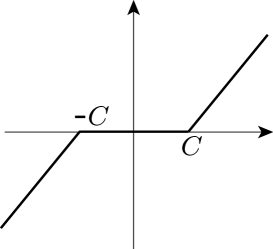
Figure 1: Illustration of soft thresholding function ${\rm prox}(\cdot|\phi_{C}^{(m)})$.

Table 1: Algorithm of SpicyMKL for block 1-norm MKL

1. Choose a sequence $\gamma^{(t)}\to\infty$ as $t\to\infty$. 2. Minimize the augmented Lagrangian with respect to $\rho$:   2. $\rho^{(t)}\!=\!\mathop{\mathop{\mathrm{argmin}}}_{\rho}\left(\!L^{\ast}(-\rho)\!+\!\!\frac{1}{2\gamma^{(t)}}\sum_{m}\|{\rm prox}(\alpha_{m}^{(t)}+\gamma^{(t)}\rho^{(t)}|\phi_{\gamma^{(t)}C}^{(m)})\|_{K_{m}}^{2}\!\!+\frac{1}{2\gamma^{(t)}}(b^{(t)}+\gamma^{(t)}\sum_{i}\rho_{i})^{2}\right).$ 3. Update $\alpha_{m}^{(t+1)}\leftarrow{\rm prox}(\alpha_{m}^{(t)}+\gamma^{(t)}\rho^{(t)}|\phi_{\gamma^{(t)}C}^{(m)}),~{}b^{(t+1)}\leftarrow b^{(t)}+\gamma^{(t)}\sum_{i}\rho_{i}^{(t)}.$ 4. Repeat 2. and 3. until the stopping criterion is satisfied.

Quick overview of the derivation of the iteration (10)-(12).

Consider the following Lagrangian of the proximal MKL problem (8):

$$\mathcal{L} =L(z)+\phi_{C}(\alpha)+\frac{\|\alpha-\alpha^{(t)}\|_{\bar{K}}^{2}}{2\gamma^{(t)}}+\frac{(b-b^{(t)})^{2}}{2\gamma^{(t)}}+\rho^{\top}(z-\bar{K}\alpha-b\mathbf{1}),$$ (14)

where $\rho\in{\mathbb{R}}^{N}$ is the Lagrangian multiplier corresponding to the equality constraint $z=\bar{K}\alpha+b\mathbf{1}$. The vector $\rho^{(t)}$ in the first step (10) is the optimal Lagrangian multiplier that maximizes the dual of the proximal MKL problem (8) (see Eq. (25)). The remaining steps (11)–(12) can be obtained by minimizing the above Lagrangian with respect to $\alpha$ and $b$ for $\rho=\rho^{(t)}$, respectively.

Detailed derivation of the iteration (10)-(12).

Let’s consider the constraint reformulation of the proximal MKL problem (8) as follows:

$$\mathop{\mathrm{minimize}}_{\begin{subarray}{l}\alpha\in{\mathbb{R}}^{MN},b\in{\mathbb{R}}\\ z\in{\mathbb{R}}^{N}\end{subarray}}\quad L(z)+\phi_{C}(\alpha)+\frac{\|\alpha-\alpha^{(t)}\|_{\bar{K}}^{2}}{2\gamma^{(t)}}+\frac{(b-b^{(t)})^{2}}{2\gamma^{(t)}},$$

subject to $$z=\bar{K}\alpha+b\mathbf{1}.$$

The Lagrangian of the above constrained minimization problem can be written as in Eq. (14).

The dual problem can be derived by minimizing the Lagrangian (14) with respect to the primal variables $(z,\alpha,b)$. See Eq. (25) for the final expression. Note that the minimization is separable into minimization with respect to $z$ (Eq. (15)), $\alpha$ (Eq. (20)), and $b$ (Eq. (24)).

First, minimizing the Lagrangian with respect to $z$ gives

$$\min_{z\in{\mathbb{R}}^{N}}\left(L(z)+\rho^{\top}z\right)=-L^{\ast}(-\rho),$$ (15)

where $L^{\ast}$ is the convex conjugate of the loss function $L$ as follows:

$$L^{\ast}(-\rho) :=\sup_{z\in{\mathbb{R}}^{N}}\left((-\rho)^{\top}z-L(z)\right)$$

$$=\sum_{i=1}^{N}\left(-\rho_{i}z_{i}-\ell(y_{i},z_{i})\right)$$

$$=\sum_{i=1}^{N}\ell^{\ast}(y_{i},-\rho_{i}),$$

where $\ell^{\ast}$ is the convex conjugate of the loss $\ell$ with respect to the second argument.

For example, the conjugate loss $\ell_{L}^{\ast}$ for the logistic loss $\ell_{L}$ is the negative entropy function as follows:

$$\ell_{L}^{\ast}(y,-\rho) =\begin{cases}(y\rho)\log(y\rho)+(1-y\rho)\log(1-y\rho)&(\textrm{if $0\leq y\rho\leq 1$}),\\ +\infty&(\textrm{otherwise}).\end{cases}$$ (16)

The conjugate loss $\ell_{H}^{\ast}$ for the hinge loss $\ell_{H}$ is given as follows:

$$\ell_{H}^{\ast}(y,-\rho) =\begin{cases}-y\rho&(\textrm{if $0\leq y\rho\leq 1$}),\\ +\infty&(\textrm{otherwise}).\end{cases}$$ (17)

Second, minimizing the Lagrangian (14) with respect to $\alpha$, we obtain

$$\min_{\alpha\in{\mathbb{R}}^{MN}}\left(\phi_{C}(\alpha)+\frac{\|\alpha-\alpha^{(t)}\|_{\bar{K}}^{2}}{2\gamma^{(t)}}-\rho^{\top}\bar{K}\alpha\right)$$

$$=\min_{\alpha\in{\mathbb{R}}^{MN}}\left(\phi_{C}(\alpha)+\frac{\|\alpha-\alpha^{(t)}-\gamma^{(t)}\rho\|_{\bar{K}}^{2}}{2\gamma^{(t)}}\right)-\frac{\|\alpha^{(t)}+\gamma^{(t)}\rho\|_{\bar{K}}^{2}}{2\gamma^{(t)}}+{\rm const}$$ (18)

$$\mathop{=}^{\eqref{eq:Aphistar},\eqref{eq:MoreauConvolution}}-\frac{1}{\gamma^{(t)}}\min_{u\in{\mathbb{R}}^{MN}}\left(\delta_{\gamma^{(t)}C}(u)+\frac{\|u-\alpha^{(t)}-\gamma^{(t)}\rho\|_{\bar{K}}^{2}}{2}\right)+{\rm const}$$ (19)

$$\mathop{=}^{\eqref{eq:Phi-l1}}-\frac{1}{\gamma^{(t)}}\sum_{m=1}^{M}\Phi_{\gamma^{(t)}C}^{(m)}(\alpha_{m}+\gamma^{(t)}\rho)+{\rm const.},$$ (20)

where ${\rm const}$ is a term that only depends on $\alpha^{(t)}$ and $\gamma^{(t)}$; the function $\delta_{C}:{\mathbb{R}}^{MN}\rightarrow{\mathbb{R}}$ is the convex conjugate of the regularization term $\phi_{C}^{(m)}(\alpha_{m})=C\|\alpha_{m}\|_{K_{m}}$ as follows:

$$\delta_{C}(u) :=\sum_{m=1}^{M}\delta_{C}^{(m)}(u_{m}),$$

where

$$\delta_{C}^{(m)}(u_{m}) :=\sup_{\alpha_{m}\in{\mathbb{R}}^{N}}\left(\left\langle u_{m},\alpha_{m}\right\rangle_{K_{m}}-\phi_{C}^{(m)}(\alpha_{m})\right)$$

$$=\sup_{\alpha_{m}\in{\mathbb{R}}^{N}}\left(\|u_{m}\|_{K_{m}}\|\alpha_{m}\|_{K_{m}}-C\|\alpha_{m}\|_{K_{m}}\right)$$

$$=\begin{cases}0&(\textrm{if $\|u_{m}\|_{K_{m}}\leq C$}),\\ +\infty&(\textrm{otherwise}).\end{cases}$$ (21)

See Fig. 2 for a one dimensional illustration of the conjugate regularizer $\delta_{C}^{(m)}$. In addition, the function $\Phi_{C}^{(m)}$ in the last line is Moreau’s envelope function (see Fig. 2):

$$\Phi_{C}^{(m)}(v_{m}) :=\min\limits_{v^{\prime}_{m}\in{\mathbb{R}}^{N}}\left(\delta_{C}^{(m)}(v^{\prime}_{m})+\frac{1}{2}\|v^{\prime}_{m}-v_{m}\|_{K_{m}}^{2}\right),$$

$$=\left\|{\rm prox}(v_{m}|\phi_{C}^{(m)})\right\|_{K_{m}}^{2}.$$ (22)

See Eq. (13) and Figure 1 for the definition of the soft-threshold operation ${\rm prox}(\cdot|\phi_{C}^{(m)})$. Furthermore, we used the following proposition and some algebra to derive Eq. (19) from Eq. (18).

Proposition 1.

Let $f:{\mathbb{R}}^{n}\rightarrow{\mathbb{R}}$ be a closed proper convex function and $f^{\ast}$ be the convex conjugate of $f$ defined as

$$f^{\ast}(y) =\sup_{x\in{\mathbb{R}}^{n}}\left(\left\langle y,x\right\rangle_{K}-f(x)\right),$$

where $K\in{\mathbb{R}}^{n\times n}$ is a positive semidefinite matrix. Then

$$\min_{x\in{\mathbb{R}}^{n}}\left(f(x)+\frac{\|x-z\|_{K}^{2}}{2}\right)+\min_{y\in{\mathbb{R}}^{n}}\left(f^{\ast}(y)+\frac{\|y-z\|_{K}^{2}}{2}\right) =\frac{\|z\|_{K}^{2}}{2}.$$ (23)

Proof.

It is a straightforward generalization of Moreau’s theorem. See Rockafellar (1970, Theorem 31.5) and Tomioka et al. (2011). ∎

Finally, minimizing the Lagrangian (14) with respect to $b$, we obtain

$$\min_{b\in{\mathbb{R}}}\left(\frac{(b-b^{(t)})^{2}}{2\gamma^{(t)}}-b\rho^{\top}\mathbf{1}\right) =-\frac{(b^{(t)}+\gamma^{(t)}\rho^{\top}\mathbf{1})^{2}}{2\gamma^{(t)}}+{\rm const},$$ (24)

where const is a term that only depends on $b^{(t)}$ and $\gamma^{(t)}$.

Combining Eqs. (15), (20), and (24), the dual of the proximal MKL problem (8) can be obtained as follows:

$$\mathop{\mathrm{maximize}}_{\rho\in{\mathbb{R}}^{N}}\quad -L^{\ast}(-\rho)-\frac{1}{2\gamma^{(t)}}\sum_{m=1}^{M}\left\|{\rm prox}(\alpha_{m}^{(t)}+\gamma^{(t)}\rho|\phi_{\gamma C}^{(m)})\right\|_{K_{m}}^{2}-\frac{1}{2\gamma^{(t)}}\left(b^{(t)}+\gamma^{(t)}\textstyle\sum_{i=1}^{N}\rho_{i}\right)^{2},$$ (25)

where the constant terms are ignored. We denote the maximand in the above dual problem by $-\varphi_{\gamma^{(t)}}(\rho;\alpha^{(t)},b^{(t)})$; see Eq. (10).

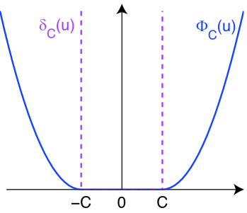
Figure 2: Comparison of the conjugate regularizer $\delta_{C}^{(m)}$ and the corresponding Moreau’s envelope function $\Phi_{C}^{(m)}$ in one dimension. The conjugate regularizer $\delta_{C}^{(m)}$ (21) is nondifferentiable at the boundary of its domain, whereas its envelope function $\Phi_{C}^{(m)}$ is smooth.

3.3 Minimizing the inner objective function

The inner objective function (25) that we need to minimize at every iteration is convex and differentiable when $L^{\ast}$ is differentiable. In fact, the gradient and the Hessian of the inner objective $\varphi_{\gamma}$ can be written as follows:

$$\nabla_{\rho}\varphi_{\gamma}(\rho;\alpha,b)=-\nabla_{\rho}L^{\ast}(-\rho)+(b+\gamma\sum_{i}\rho_{i}){\bm{1}}+\sum_{m\in M_{+}}K_{m}{\rm prox}\left(\alpha_{m}+\gamma\rho\Big{|}\phi_{\gamma C}^{(m)}\right),$$ (26)

$$\nabla^{2}_{\rho}\varphi_{\gamma}(\rho;\alpha,b)=\nabla^{2}_{\rho}L^{\ast}(-\rho)+\gamma{\bm{1}}{\bm{1}}^{\top}+\gamma\!\!\!\!\sum_{m\in M_{+}}\!\!\!\!\left((1-q_{m})K_{m}\!\!+\!q_{m}K_{m}\tilde{v}_{m}\tilde{v}_{m}^{\top}K_{m}\right),$$ (27)

where $M_{+}$ is the set of indices corresponding to the active kernels; i.e., $M_{+}=\{m\in\{1,\ldots,M\}\mid\|\alpha_{m}+\gamma\rho\|_{K_{m}}>\gamma C\}$; for $m\in M_{+}$, a scalar $q_{m}$ and a vector $\tilde{v}_{m}\in{\mathbb{R}}^{N}$ are defined as $q_{m}:=\frac{\gamma C}{\|\alpha_{m}+\gamma\rho\|_{K_{m}}}$ and $\tilde{v}_{m}:=(\alpha_{m}+\gamma\rho)/\|\alpha_{m}+\gamma\rho\|_{K_{m}}$.

Remark 1.

The computation of the objective $\varphi_{\gamma}(\rho;\alpha,b)$ (25), the gradient (26), and the Hessian (27) is efficient because they require only the terms corresponding to the active kernels $\{k_{m}\mid m\in M_{+}\}$.

The above sparsity, which makes the proposed algorithm efficient, comes from our dual formulation. By taking the dual, there appears flat region (see Fig. 2); i.e. the region $\{\rho\mid{\rm prox}(\alpha_{m}^{(t)}+\gamma^{(t)}\rho|\phi_{\gamma^{(t)}C}^{(m)})=0\}$ is not a single point but has its interior.

Since the inner objective function (25) is differentiable, and the sparsity of the intermediate solution can be exploited to evaluate the gradient and Hessian of the inner objective, the inner minimization can efficiently be carried out. We call the proposed algorithm Sparse Iterative MKL (SpicyMKL). The update equations (11)-(12) exactly correspond to the augmented Lagrangian method for the dual of the problem (7) (see Tomioka and Sugiyama (2009)) but derived in more general way using the techniques from Rockafellar (1976).

We use the Newton method with line search for the minimization of the inner objective (25). The line search is used to keep $\rho$ inside the domain of the dual loss $L^{\ast}$. This works when the gradient of the dual loss $L^{\ast}$ is unbounded at the boundary of its domain, for example the logistic loss (16), in which case the minimum is never attained at the boundary. On the other hand, for the hinge loss (17), the solution lies typically at the boundary of the domain $0\leq y\rho\leq 1$. This situation is handled separately in the next subsection.

3.4 Explicitly handling boundary constraints

The Newton method with line search described in the last section is unsuitable when the conjugate loss function $\ell^{\ast}(y,\cdot)$ has a non-differentiable point in the interior of its domain or it has finite gradient at the boundary of its domain. We use the same augmented Lagrangian technique for these cases. More specifically we introduce additional primal variables so that the AL function $\varphi_{\gamma}(\cdot;\alpha,b)$ becomes differentiable. First we explain this in the case of hinge loss for classification. Next we discuss a generalization to other cases.

3.4.1 Optimization for hinge loss

Here we explain how the augmented Lagrangian technique is applied to the hinge loss. To this end, we introduce two sets of slack variables $\xi=(\xi_{1},\ldots,\xi_{N})^{\top}\geq 0,\zeta=(\zeta_{1},\ldots,\zeta_{N})^{\top}\geq 0$ as in standard SVM literature (see e.g., Schölkopf and Smola (2002)). The basic update equation (Eq. (8)) is rewritten as follows:

$$(\alpha^{(t+1)},b^{(t+1)},\xi^{(t+1)},\zeta^{(t+1)})=\!\!\!\!\!\!$$

$$\mathop{\mathrm{argmin}}\limits_{\begin{subarray}{l}\alpha\in{\mathbb{R}}^{(MN)},b\in{\mathbb{R}}\\ \xi\in\mathbb{R}_{+}^{N},\zeta\in\mathbb{R}_{+}^{N}\end{subarray}}\Biggl{\{}H_{C}(\alpha,b,\xi,\zeta)+\frac{1}{2\gamma^{(t)}}\left(\|\alpha-\alpha^{(t)}\|_{\bar{K}}^{2}+(b-b^{(t)})^{2}+\|\xi-\xi^{(t)}\|^{2}+\|\zeta-\zeta^{(t)}\|^{2}\right)\Biggr{\}},$$

where

$$H_{C}(\alpha,b,\xi,\zeta)=\begin{cases}\sum_{i=1}^{N}\xi_{i}+\phi_{C}(\alpha)&\Big{(}\textrm{if }y_{i}(\displaystyle(\sum_{m=1}^{M}K_{m}\alpha_{m})_{i}+b)=1-\xi_{i}+\zeta_{i},~{}\xi_{i}\geq 0,~{}\zeta_{i}\geq 0,\forall i\Big{)},\\ \textstyle+\infty&\textrm{(otherwise).}\end{cases}$$

This function $$H_{C} \rho\in{\mathbb{R}}^{N} u\in{\mathbb{R}}^{MN}$$ can again be expressed in terms of maximum over , as follows:

$$H_{C}(\alpha,b,\xi,\zeta)$$

$$=\max_{\rho\in{\mathbb{R}}^{N},u\in{\mathbb{R}}^{MN}}\Biggl{\{}-\sum_{i=1}^{N}(-y_{i}\rho_{i})-b\sum_{i=1}^{N}\rho_{i}-\sum_{m=1}^{M}\delta_{C}^{m}(u_{m})-\sum_{m=1}^{M}\langle\alpha_{m},\rho-u_{m}\rangle_{K_{m}}$$

$$~{}~{}~{}~{}~{}~{}~{}~{}~{}~{}~{}~{}~{}~{}~{}~{}~{}~{}~{}~{}~{}~{}+\sum_{i=1}^{N}\xi_{i}(1-y_{i}\rho_{i})+\sum_{i=1}^{N}\zeta_{i}(y_{i}\rho_{i})\Biggr{\}}.$$

We exchange the order of minimization and maximization as before and remove $\alpha,b,\xi,\zeta$, and $u_{m}$ by explicitly minimizing or maximizing over them (see also Section 3.2). Finally we obtain the following update equations.

$$\textstyle\alpha_{m}^{(t+1)} \textstyle={\rm prox}(\alpha_{m}^{(t)}+\gamma^{(t)}\rho^{(t)}|\phi_{\gamma^{(t)}C}^{(m)}),$$ (28)

$$\textstyle b^{(t+1)} =b^{(t)}+\gamma^{(t)}\sum_{i=1}^{N}\rho_{i}^{(t)},$$ (29)

$$\textstyle\xi_{i}^{(t+1)} \textstyle=\max(0,\xi_{i}^{(t)}-\gamma_{\xi}^{(t)}(1-y_{i}\rho_{i}^{(t)})),$$ (30)

$$~{}~{}~{}~{}\textstyle\zeta_{i}^{(t+1)}\textstyle =\max(0,\zeta_{i}^{(t)}-\gamma_{\zeta}^{(t)}y_{i}\rho_{i}^{(t)}).$$ (31)

and $\rho^{(t)}\in{\mathbb{R}}^{N}$ is the minimizer of the function $\varphi_{\gamma^{(t)}}(\rho;\alpha^{(t)},b^{(t)},\xi^{(t)},\zeta^{(t)})$ defined as follows:

$$\textstyle\varphi_{\gamma}(\rho;\alpha,b,\xi,\zeta)= \textstyle-\sum\limits_{i=1}^{N}y_{i}\rho_{i}+\frac{1}{2\gamma}(b+\gamma\sum\limits_{i=1}^{N}\rho_{i})^{2}+\sum\limits_{m=1}^{M}\frac{1}{2\gamma}\|{\rm prox}(\alpha_{m}+\gamma\rho|\phi_{\gamma C}^{(m)})\|$$

$$\textstyle+\frac{1}{2\gamma}\sum\limits_{i=1}^{N}\max(0,\xi_{i}-\gamma(1-y_{i}\rho_{i}))^{2}+\frac{1}{2\gamma}\sum\limits_{i=1}^{N}\max(0,\zeta_{i}-\gamma y_{i}\rho_{i})^{2},$$ (32)

and $\gamma\in\mathbb{R}_{+}$. The gradient and the Hessian of $\varphi_{\gamma}$ with respect to $\rho$ can be obtained in a similar way to Eqs. (26) and (27). Thus we use the Newton method for the minimization (32). The overall algorithm is analogous to Table 1 with update equations (28)-(32).

3.4.2 Optimization for general loss functions with constraints

Here we generalize the above argument to a broader class of loss functions. We assume that the dual of the loss function can be written by using twice differentiable convex functions $\ell_{0}$ and $h_{j}$ as

$$\ell^{\ast}(y_{i},\rho_{i})=\min_{\tilde{\rho}}\{\ell_{0}^{\ast}(y_{i},(\rho_{i},\tilde{\rho}_{i}))\mid h_{j}(y_{i},(\rho_{i},\tilde{\rho}_{i}))\leq 0~{}(1\leq j\leq B)\},.$$ (33)

where $\tilde{\rho}_{i}\in{\mathbb{R}}^{B^{\prime}}$ is an auxiliary variable. An example is $\epsilon$-sensitive loss for regression that is defined as

$$\ell(y,f)=\begin{cases}|f-y|-\epsilon&(\text{if}~{}|f-y|\geq\epsilon)\\ 0&(\text{otherwise})\end{cases}.$$

By simple calculation, the dual function of the $\epsilon$-sensitive loss is given as

$$\ell^{*}(y,\rho)=\begin{cases}y\rho+|\rho|\epsilon&(\text{if}~{}|\rho|\leq 1)\\ \infty&(\text{otherwise})\\ \end{cases},$$ (34)

This is not differentiable, but is written as

$$\ell^{*}(y,\rho)=\min_{\tilde{\rho}}\{y\rho+(\rho+2\tilde{\rho})\epsilon\mid\rho-1\leq 0,~{}-1-\rho\leq 0,~{}-\tilde{\rho}\leq 0,~{}-\rho-\tilde{\rho}\leq 0\}.$$ (35)

Thus in this example, $\ell_{0}^{\ast}(y,(\rho,\tilde{\rho}))=y\rho+(\rho+2\tilde{\rho})$, $h_{1}(y,(\rho,\tilde{\rho}))=\rho-1$, $h_{2}(y,(\rho,\tilde{\rho}))=-1-\rho$, $h_{3}(y,(\rho,\tilde{\rho}))=-\tilde{\rho}$, and $h_{4}(y,(\rho,\tilde{\rho}))=-\rho-\tilde{\rho}$ in the formulation of Eq. (33).

The update equation becomes as following:

$$(\alpha^{(t+1)},b^{(t+1)},\xi^{(t+1)})=\!\!\!\!\!\!$$ (36)

$$\mathop{\mathrm{argmin}}\limits_{\begin{subarray}{l}\alpha\in{\mathbb{R}}^{(MN)},b\in{\mathbb{R}}\\ \xi\in\mathbb{R}_{+}^{NB}\end{subarray}}\Biggl{\{}H_{C}(\alpha,b,\xi)+\frac{1}{2\gamma^{(t)}}\left(\|\alpha-\alpha^{(t)}\|_{\bar{K}}^{2}+(b-b^{(t)})^{2}+\|\xi-\xi^{(t)}\|^{2}\right)\Biggr{\}},$$ (37)

where $H_{C}$ is expressed in terms of maximum over $\rho\in{\mathbb{R}}^{N}$, $\tilde{\rho}\in{\mathbb{R}}^{NB^{\prime}}$, $u\in{\mathbb{R}}^{MN}$ as follows:

$$H_{C}(\alpha,b,\xi)$$

$$=\max_{\rho\in{\mathbb{R}}^{N},\tilde{\rho}\in{\mathbb{R}}^{NB^{\prime}},u\in{\mathbb{R}}^{MN}}\Biggl{\{}-\sum_{i=1}^{N}\ell_{0}^{\ast}(y_{i},(-\rho_{i},\tilde{\rho}_{i}))-\sum_{m=1}^{M}\delta_{C}^{m}(u_{m})-\sum_{m=1}^{M}\langle\alpha_{m},\rho-u_{m}\rangle_{K_{m}}-b\sum_{i=1}^{N}\rho_{i}$$

$$~{}~{}~{}~{}~{}~{}~{}~{}~{}~{}~{}~{}~{}~{}~{}~{}~{}~{}~{}~{}~{}~{}-\sum_{i=1}^{N}\sum_{j=1}^{B}\xi_{i,j}h_{j}(y_{i},(-\rho_{i},\tilde{\rho}_{i}))\Biggr{\}}.$$

Note that the minimum of $H_{C}(\alpha,b,\xi)$ with respect to $\xi$ is the primal objective function $L(\bar{K}\alpha+b{\bm{1}})+\phi_{C}(\alpha)$ because by exchanging $\min$ and $\max$ we have

$$\min_{\xi\in\mathbb{R}_{+}^{NB}}H_{C}(\alpha,b,\xi)$$

$$=\max_{\begin{subarray}{c}\rho\in{\mathbb{R}}^{N}\\ \tilde{\rho}\in{\mathbb{R}}^{NB^{\prime}},u\in{\mathbb{R}}^{MN}~{}~{}\end{subarray}}\inf_{\xi\in\mathbb{R}_{+}^{NB}}\Biggl{\{}-\sum_{i=1}^{N}\ell_{0}^{\ast}(y_{i},(-\rho_{i},\tilde{\rho}_{i}))-\sum_{m=1}^{M}\delta_{C}^{m}(u_{m})-\sum_{m=1}^{M}\langle\alpha_{m},\rho-u_{m}\rangle_{K_{m}}-b\sum_{i=1}^{N}\rho_{i}$$

$$~{}~{}~{}~{}~{}~{}~{}~{}~{}~{}~{}~{}~{}~{}~{}~{}~{}~{}~{}~{}~{}~{}~{}~{}~{}~{}~{}~{}-\sum_{i=1}^{N}\sum_{j=1}^{B}\xi_{i,j}h_{j}(y_{i},(-\rho_{i},\tilde{\rho}_{i}))\Biggr{\}}$$

$$=\max_{\rho\in{\mathbb{R}}^{N}\tilde{\rho}\in{\mathbb{R}}^{NB^{\prime}}}\Biggl{\{}-\sum_{i=1}^{N}\ell_{0}^{\ast}(y_{i},(-\rho_{i},\tilde{\rho}_{i}))+\rho^{\top}(\bar{K}\alpha+b{\bm{1}})\mid h_{j}(y_{i},(-\rho_{i},\tilde{\rho}_{i}))\leq 0~{}(\forall i,j)\Biggr{\}}$$

$$~{}~{}~{}~{}~{}~{}+\max_{u\in{\mathbb{R}}^{MN}}\left\{-\sum_{m=1}^{M}\delta_{C}^{m}(u_{m})+\sum_{m=1}^{M}\langle\alpha_{m},u_{m}\rangle_{K_{m}}\right\}$$

$$=L(\bar{K}\alpha+b{\bm{1}})+\phi_{C}(\alpha).$$

However it is difficult to directly optimize the primal objective. Therefore we add the penalty term as in Eq. (37) and solve its dual problem. We exchange the order of minimization and maximization as in the last section (see also Section 3.2) and remove $\alpha,b,\xi$, and $u_{m}$ by explicitly minimizing or maximizing over them. Finally we obtain the following update equations.

$$\textstyle\alpha_{m}^{(t+1)} \textstyle={\rm prox}(\alpha_{m}^{(t)}+\gamma^{(t)}\rho^{(t)}|\phi_{\gamma^{(t)}C}^{(m)}),$$ (38)

$$\textstyle b^{(t+1)} =b^{(t)}+\gamma^{(t)}\sum_{i=1}^{N}\rho_{i}^{(t)}$$ (39)

$$\textstyle\xi_{i,j}^{(t+1)} \textstyle=\max(0,\xi_{i,j}^{(t)}-\gamma^{(t)}h_{j}(y_{i},(-\rho_{i}^{(t)},\tilde{\rho}_{i}^{(t)}))).$$ (40)

where $(\rho^{(t)},\tilde{\rho}^{(t)})\in{\mathbb{R}}^{N}\times{\mathbb{R}}^{NB^{\prime}}$ is the minimizer of the function $\varphi_{\gamma^{(t)}}(\rho,\tilde{\rho};\alpha^{(t)},b^{(t)},\xi^{(t)})$ defined as follows:

$$\textstyle\varphi_{\gamma}(\rho,\tilde{\rho};\alpha,b,\xi)= \textstyle\sum\limits_{i=1}^{N}\ell_{0}^{\ast}(y_{i},(-\rho_{i},\tilde{\rho}_{i}))+\frac{1}{2\gamma}(b+\gamma\sum\limits_{i=1}^{N}\rho_{i})^{2}+\sum\limits_{m=1}^{M}\frac{1}{2\gamma}\|{\rm prox}(\alpha_{m}+\gamma\rho|\phi_{\gamma C}^{(m)})\|_{K_{m}}^{2}$$

$$\textstyle+\frac{1}{2\gamma}\sum\limits_{i=1}^{N}\sum\limits_{j=1}^{B}\max(0,\xi_{i,j}-\gamma h_{j}(y_{i},(-\rho_{i},\tilde{\rho}_{i})))^{2},$$ (41)

and $\gamma\in\mathbb{R}_{+}$. The gradient and the Hessian of $\varphi_{\gamma}$ with respect to $(\rho,\tilde{\rho})$ can be obtained in a similar way to Eqs. (26) and (27). Thus we use the Newton method for the minimization (32). The overall algorithm is summarized in Table 2.

Table 2: Algorithm of SpicyMKL for a general regularization term and a general loss function

1. Choose a sequence $\gamma^{(t)}\to\infty$ as $t\to\infty$. 2. Minimize the augmented Lagrangian with respect to $\rho$ and $\tilde{\rho}$:   2. $(\rho^{(t)},\tilde{\rho}^{(t)})\!=\!\mathop{\mathop{\mathrm{argmin}}}_{\rho,\tilde{\rho}}\Big{(}\!\sum_{i}\ell_{0}^{\ast}(y_{i},(-\rho_{i},\tilde{\rho}_{i}))\!+\!\frac{1}{2\gamma^{(t)}}\sum_{m}\|{\rm prox}(\alpha_{m}^{(t)}+\gamma^{(t)}\rho|\phi_{\gamma^{(t)}C}^{(m)})\|_{K_{m}}^{2}\!\!$                     $+\frac{1}{2\gamma^{(t)}}\sum\limits_{i=1}^{N}\sum\limits_{j=1}^{B}\max(0,\xi_{i,j}^{(t)}-\gamma h_{j}(y_{i},(-\rho_{i},\tilde{\rho}_{i})))^{2}+\frac{1}{2\gamma^{(t)}}(b^{(t)}+\gamma^{(t)}\sum_{i}\rho_{i})^{2}\Big{)}.$ 3. Update $\alpha_{m}^{(t+1)}\leftarrow{\rm prox}(\alpha_{m}^{(t)}+\gamma^{(t)}\rho^{(t)}|\phi_{\gamma^{(t)}C}^{m}),~{}b^{(t+1)}\leftarrow b^{(t)}+\gamma^{(t)}\sum_{i}\rho_{i}^{(t)},$        $\xi_{i,j}^{(t+1)}\leftarrow\max(0,\xi_{i,j}^{(t)}-\gamma^{(t)}h_{j}(y_{i},(\rho_{i}^{(t)},\tilde{\rho}_{i}^{(t)}))).$ 4. Repeat 2. and 3. until the stopping criterion is satisfied.

3.5 Technical details of computations

3.5.1 Back-tracking in the Newton update

We use back-tracking line search with Armijo’s rule to find a step size of the Newton method. During the back-tracking, the computational bottle-neck is the computation of the norm $\|\rho+c\Delta\rho+\frac{\alpha_{m}}{\gamma_{m}}\|_{K_{m}}$ $(m=1,\dots,M)$ where $\Delta\rho$ is the Newton update direction and $0<c\leq 1$ is a step size. However, the above computation is necessary only for the active kernels $M_{+}$; for example, the active kernels $M_{+}$ is included in $\{m\mid\|\rho+\frac{\alpha_{m}}{\gamma_{m}}\|_{K_{m}}>C$ or $\|\rho+\Delta\rho+\frac{\alpha_{m}}{\gamma_{m}}\|_{K_{m}}>C\}$ for block 1-norm MKL and $\{m\mid\|\rho\|_{K_{m}}>(1-\lambda)C$ or $\|\rho+\Delta\rho\|_{K_{m}}>(1-\lambda)C\}$ for Elastic-net MKL because of the convexity of $\|\cdot\|_{K_{m}}$. This reduces the computation time considerably.

3.5.2 Parallelization in the computation of $\big{\|}\alpha_{m}^{(t)}+\frac{\rho^{(t)}}{\gamma^{(t)}_{m}}\big{\|}_{K_{m}}$

The computation of $\big{\|}\alpha_{m}^{(t)}+\frac{\rho^{(t)}}{\gamma^{(t)}_{m}}\big{\|}_{K_{m}}$ for $m=1,\dots,M$ is necessary at every outer iteration. Thus when the number of kernels is large, its cost cannot be ignored. Fortunately, the computation with respect to the $m$-th kernel is independent of the others and the outer loop is easily parallelizable. In our experiments, we implemented the parallel computing by OpenMP in mex-files of our Matlab^\tiny{R}⃝ code. We observed twenty or thirty percent improvement of overall computational time by the parallelization.

4 Generalized block-norm formulation

Motivated by the recent interest in non-sparse regularization for MKL, we consider a generalized block norm formulation in this section. The proposed formulation uses a concave function $g$ and it subsumes previously proposed MKL models, such as $\ell_{p}$-norm MKL (Kloft et al., 2009) and Elastic-net MKL (Tomioka and Suzuki, 2009), as different choices of the concave function $g$. Moreover, using a convex upper-bounding technique (Palmer et al., 2006) we show that the proposed formulation can be written also as a Tikhonov regularization problem (3). Thus the solution can be easily mapped to kernel weights as in previous approaches. We extend SpicyMKL algorithm for the generalized formulation in Section 4.2. Furthermore we preset an efficient one-step optimization procedure for Elastic-net MKL and $\ell_{p}$-norm MKL in Section 4.3.

4.1 Proposed formulation

We consider the following generalized block-norm formulation:

$$\mathop{\mathrm{minimize}}_{f_{1}\in{\mathcal{H}}_{1},\ldots,f_{M}\in{\mathcal{H}}_{M},b\in{\mathbb{R}}} \sum_{i=1}^{N}\ell\left(y_{i},\textstyle\sum_{m=1}^{M}f_{m}(x_{i})+b\right)+C\sum_{m=1}^{M}g(\|f_{m}\|_{{\mathcal{H}}_{m}}^{2}),$$ (42)

where $g$ is a non-decreasing concave function defined on the nonnegative reals, and we assume that $\tilde{g}(x)=g(x^{2})$ is a convex function of $x$. For example, taking $g(x)=\sqrt{x}$ gives the block 1-norm MKL in Eq. (4) and taking $g(x)=x^{q/2}/q$ gives the block $q$-norm MKL (Kloft et al., 2009; Nath et al., 2009). Moreover by choosing $g(x)=(1-\lambda)\sqrt{x}+\frac{\lambda}{2}x$, we obtain the following Elastic-net MKL (Tomioka and Suzuki, 2009):

$$\mathop{\mathrm{minimize}}_{f_{1}\in{\mathcal{H}}_{1},\ldots,f_{M}\in{\mathcal{H}}_{M},b\in{\mathbb{R}}} \sum_{i=1}^{N}\ell\left(y_{i},\textstyle\sum_{m=1}^{M}f_{m}(x_{i})+b\right)+C\sum_{m=1}^{M}\left((1-\lambda)\|f_{m}\|_{{\mathcal{H}}_{m}}+\frac{\lambda}{2}\|f_{m}\|_{{\mathcal{H}}_{m}}^{2}\right),$$ (43)

which reduces to the block 1-norm regularization (4) for $\lambda=0$ and the uniform-weight combination ($d_{m}=1$ ($\forall m$) in Eq. (2)) for $\lambda=1$.

Note that the generalized regularization term in the above formulation (42) is separable into each kernel component; thus it can be more efficiently handled than the squared regularization used in previous studies (Kloft et al., 2009, 2010).

The first question we need to answer is how the generalized block-norm formulation (42) is related to the Tikhonov regularization formulation (3). This can be shown using a convex upper-bounding technique; see (Palmer et al., 2006). For any given concave function $g$, the concave conjugate $g^{\ast}$ of $g$ is defined as follows:

$$g^{\ast}(y)=\inf_{x\geq 0}\left(xy-g(x)\right).$$

The definition of concave conjugate immediately implies that the following inequality is true:

$$g\left(\|f_{m}\|_{{\mathcal{H}}_{m}}^{2}\right) \leq\frac{\|f_{m}\|_{{\mathcal{H}}_{m}}^{2}}{2d_{m}}-g^{\ast}\left(\frac{1}{2d_{m}}\right).$$

Note that the equality is obtained by taking $d_{m}=1/(2g^{\prime}(\|f_{m}\|_{{\mathcal{H}}_{m}}^{2}))$, where $g^{\prime}$ is the derivative of $g$. Therefore, the generalized block-norm formulation (42) is equivalent to the following Tikhonov regularization problem:

$$\mathop{\mathrm{minimize}}_{\begin{subarray}{c}f_{1}\in{\mathcal{H}}_{1},\ldots,f_{M}\in{\mathcal{H}}_{M},\\ b\in{\mathbb{R}},\\ d_{1}\geq 0,\ldots,d_{M}\geq 0\end{subarray}} \sum_{i=1}^{N}\ell\left(y_{i},\textstyle\sum_{m=1}^{M}f_{m}(x_{i})+b\right)+\frac{C}{2}\sum_{m=1}^{M}\left(\frac{\|f_{m}\|_{{\mathcal{H}}_{m}}^{2}}{d_{m}}+h(d_{m})\right),$$ (44)

where we define the regularizer $h(d_{m})=-2g^{\ast}(1/(2d_{m}))$. It is easy to obtain the regularizer $h$ corresponding to the block 1-norm MKL, block $q$-norm MKL, and the Elastic-net MKL, and it is shown in Table 3. See Tomioka and Suzuki (2011) for more detailed and generalized discussions about the relations between the regularizations on the RKHS norm $\{\|f_{m}\|_{{\mathcal{H}}_{m}}\}_{m}$ and the kernel weight $\{d_{m}\}_{m}$.

Once we obtain the optimizer $\{f^{*}_{m}\}_{m}$ for the generalized block-norm formulation (42), then we can easily recover the corresponding kernel weight by the relation

$$d_{m}=\frac{1}{2g^{\prime}(\|f_{m}^{*}\|_{{\mathcal{H}}_{m}}^{2})}=\frac{1}{2g^{\prime}(\|\alpha_{m}^{*}\|_{K_{m}}^{2})},$$

where $\alpha_{m}^{*}$ is the optimal coefficient vector corresponding to $f^{*}_{m}$. For the Elastic-net MKL, for example, the kernel weight is recovered as

$$d_{m}=\begin{cases}0,&(\|\alpha_{m}^{*}\|_{K_{m}}=0),\\ \frac{\|\alpha_{m}^{*}\|_{K_{m}}}{1-\lambda+\lambda\|\alpha_{m}^{*}\|_{K_{m}}},&(\text{otherwise}).\end{cases}$$

Note that we have a freedom of a constant multiplication for the kernel weight.

Table 3: Correspondence of the concave function $g$ in Eq. (42) and the regularizer $h$ in Eq. (44). For block $q$-norm MKL, the exponent $q$ in the block norm formulation and the exponent $p$ in the Tikhonov regularization problem correspond as $p:=q/(q-2)$. $I_{[0,1]}$ denotes the indicator function of the interval $[0,1]$; i.e., $I_{[0,1]}(x)=0$ (if $x\in[0,1]$), and $I_{[0,1]}(x)=\infty$ (otherwise).

MKL model	$g(x)$	$h(d_{m})$
block 1-norm MKL	$\sqrt{x}$	$d_{m}$
block $q$-norm MKL	$\frac{1}{q}x^{q/2}$	$\frac{1}{p}d_{m}^{p}$
Elastic-net MKL	$(1-\lambda)\sqrt{x}+\frac{\lambda}{2}x$	$\frac{(1-\lambda)^{2}d_{m}}{1-\lambda d_{m}}$
Uniform-weight MKL	$x/2$	$I_{[0,1]}(d_{m})$

4.2 SpicyMKL for generalized block-norm formulation

Now we are ready to extend SpicyMKL algorithm to the generalized block-norm formulation (42). The original iteration (10)-(12) needs three modifications, namely the proximity operator ${\rm prox}(\cdot|\phi_{C}^{(m)})$, the conjugate regularizer $\delta_{C}^{(m)}$, and Moreau’s envelope function $\Phi_{C}^{(m)}$.

First the proximity operator ${\rm prox}(\cdot|\phi_{C}^{(m)})$ is redefined using the generalized regularization term $g(\|\cdot\|_{K_{m}}^{2})$ as follows:

$${\rm prox}(v_{m}|\phi_{C}^{(m)}) :=\mathop{\mathrm{argmin}}_{v_{m}^{\prime}\in{\mathbb{R}}^{N}}\left(Cg(\|v_{m}^{\prime}\|_{K_{m}}^{2})+\frac{1}{2}\|v_{m}^{\prime}-v_{m}\|_{K_{m}}^{2}\right).$$

Note that the above minimization reduces to a one-dimensional minimization along $v_{m}^{\prime}=cv_{m}$. Let $\tilde{g}_{C}(x)=Cg(x^{2})$. In fact, due to the Cauchy-Schwarz inequality, we have

$$\tilde{g}_{C}(\|v_{m}^{\prime}\|_{K_{m}})+\frac{1}{2}\|v_{m}^{\prime}-v_{m}\|_{K_{m}}^{2} \geq\tilde{g}_{C}(\|v_{m}^{\prime}\|_{K_{m}})+\frac{1}{2}(\|v_{m}^{\prime}\|_{K_{m}}-\|v_{m}\|_{K_{m}})^{2}.$$

The minimum is obtained when

$$\|v_{m}^{\prime}\| ={\rm prox}(\|v_{m}\|_{K_{m}}|\tilde{g}_{C})$$

$$=\mathop{\mathrm{argmin}}_{x\geq 0}\left(\tilde{g}_{C}(x)+\frac{1}{2}(x-\|v_{m}\|_{K_{m}})^{2}\right).$$

For example, for Elastic-net MKL, the regularizer $\tilde{g}$ is written as $\tilde{g}(x)=(1-\lambda)x+\lambda x^{2}/2$, and the one dimensional proximity operator ${\rm prox}(\cdot|\tilde{g}_{C})$ is obtained as follows:

$${\rm prox}(x|\tilde{g}_{C}) =\begin{cases}0&(\textrm{if $0\leq x\leq C(1-\lambda)$}),\\ \frac{x-C(1-\lambda)}{C\lambda+1}&(\textrm{otherwise}).\end{cases}$$

Therefore, the proximity operator ${\rm prox}(v_{m}|\phi_{C}^{(m)})$ is obtained as follows:

$${\rm prox}(v_{m}|\phi_{C}^{(m)}) =\begin{cases}0&(\textrm{if $\|v_{m}\|_{K_{m}}\leq C(1-\lambda)$}),\\ \frac{\|v_{m}\|_{K_{m}}-C(1-\lambda)}{(C\lambda+1)\|v_{m}\|_{K_{m}}}v_{m}&(\textrm{otherwise}).\end{cases}$$

Second, the convex conjugate of the regularizer $\delta_{C}^{(m)}$ is redefined as follows:

$$\delta_{C}^{(m)}(u_{m}) :=\sup_{\alpha_{m}\in{\mathbb{R}}^{N}}\left(\left\langle u_{m},\alpha_{m}\right\rangle_{K_{m}}-\tilde{g}_{C}(\|\alpha_{m}\|_{K_{m}})\right)$$

$$=\sup_{\alpha_{m}\in{\mathbb{R}}^{N}}\left(\|u_{m}\|_{K_{m}}\|\alpha_{m}\|_{K_{m}}-\tilde{g}_{C}(\|\alpha_{m}\|_{K_{m}})\right)$$

$$=\tilde{g}_{C}^{\ast}(\|u_{m}\|_{K_{m}}).$$ (45)

For example, for the same Elastic-net regularizer, the convex conjugate $\tilde{g}_{C}^{\ast}(y)$ is obtained as follows:

$$\tilde{g}_{C}^{\ast}(y) =\sup_{x\geq 0}\left(xy-C(1-\lambda)x-\frac{C\lambda}{2}x^{2}\right)$$

$$=\begin{cases}0&(\textrm{if $0\leq y\leq C(1-\lambda)$}),\\ \frac{(y-C(1-\lambda))^{2}}{2C\lambda}&(\textrm{otherwise}).\end{cases}$$ (46)

Third the envelope function $\Phi_{C}^{(m)}$ is redefined in terms of the above new conjugate regularizer $\delta_{C}^{(m)}$ as follows:

$$\Phi_{C}^{(m)}(v_{m}) :=\min_{v_{m}^{\prime}\in{\mathbb{R}}^{N}}\left(\tilde{g}^{\ast}_{C}(\|v_{m}^{\prime}\|_{K_{m}})+\frac{1}{2}\|v_{m}^{\prime}-v_{m}\|_{K_{m}}^{2}\right)$$

$$=\min_{v_{m}^{\prime}\in{\mathbb{R}}^{N}}\left(\tilde{g}^{\ast}_{C}(\|v_{m}^{\prime}\|_{K_{m}})+\frac{1}{2}(\|v_{m}^{\prime}\|_{K_{m}}-\|v_{m}\|_{K_{m}})^{2}\right)$$

$$=\widehat{\tilde{g}_{C}^{\ast}}(\|v_{m}\|_{K_{m}}),$$

where we again used Cauchy-Schwarz inequality in the second line, and $\widehat{\tilde{g}_{C}^{\ast}}$ is the Moreau’s envelope function of $\tilde{g}^{\ast}_{C}$ as follows:

$$\widehat{\tilde{g}_{C}^{\ast}}(y)=\min_{y^{\prime}\geq 0}\left(\tilde{g}_{C}^{\ast}(y^{\prime})+\frac{1}{2}(y^{\prime}-y)^{2}\right).$$

With the above three modifications, the SpicyMKL iteration is rewritten as follows:

$$\rho^{(t)} :=\mathop{\mathrm{argmin}}_{\rho\in{\mathbb{R}}^{N}}\left(L^{\ast}(-\rho)+\frac{1}{\gamma^{(t)}}\sum_{m=1}^{M}\widehat{\tilde{g}^{\ast}_{C}}(\|\alpha_{m}+\gamma^{(t)}\rho\|_{K_{m}})+\frac{1}{2\gamma^{(t)}}(b+\gamma^{(t)}\textstyle\sum\limits_{i=1}^{N}\rho_{i})^{2}\right),$$ (47)

$$\alpha_{m}^{(t+1)} ={\rm prox}\left(\alpha_{m}^{(t)}+\gamma^{(t)}\rho^{(t)}\Big{|}\phi_{\gamma^{(t)}C}^{(m)}\right)\qquad(m=1,\ldots,M),$$

$$b^{(t+1)} =b^{(t)}+\gamma^{(t)}\sum_{i=1}^{N}\rho_{i}^{(t)}.$$

Note that if $\tilde{g}_{C}^{\ast}(0)=0$ (this is the case if $\tilde{g}_{C}(0)=0$), the envelope function $\widehat{\tilde{g}_{C}^{\ast}}(\cdot)$ in (47) becomes zero whenever the norm $\|\alpha_{m}+\gamma^{(t)}\rho\|_{K_{m}}$ is zero. Thus the inner objective (47) inherits the computational advantage provided by sparsity of the 1-norm SpicyMKL presented in Section 3.3. Moreover, the gradient and Hessian of the generalized inner objective (47) can be computed in a similar manner as (26) and (27).

A generalization to the general loss functions with constraints is also straightforward; we only need to replace $\|{\rm prox}(\alpha_{m}+\gamma\rho|\phi_{\gamma C}^{(m)})\|_{K_{m}}^{2}$ in Eq. (41) (the definition of $\varphi_{\gamma}(\rho,\tilde{\rho};\alpha,b,\xi)$) with $\widehat{\tilde{g}^{\ast}_{C}}(\|\alpha_{m}+\gamma\rho\|_{K_{m}})$.

Implementation of general loss and regularization

Our Matlab implementation is suited to general loss and block-norm regularization functions. The code runs under general settings if one plugs in scripts of the following information: the primal and dual functions of the loss, the gradient and Hessian of the dual loss, the primal and dual of the regularization function, the corresponding proximity operator and the derivative of the proximity operator.

4.3 One step optimization for a regularization function with smooth dual

When the convex conjugate $\delta_{C}^{(m)}$ of the regularization term $\phi_{C}^{(m)}$ is smooth (twice differentiable), the optimization needs only one step iteration of the outer loop. We illustrate the optimization method for smooth dual function in a generalized formulation and show two useful examples, Elastic-net MKL for $\lambda>0$ and block $q$-norm MKL for $q>1$.

The primal problem Eq. (7) is equivalent to the following dual problem by Fenchel’s duality theorem (Rockafellar, 1970, Theorem 31.2):

$$\textstyle\mathop{\mathrm{maximize}}\limits_{\begin{subarray}{c}\rho\in{\mathbb{R}}^{N}\\ {\bm{1}}^{\top}\rho=0\end{subarray}}\textstyle\bigg{(} -L^{\ast}(-\rho)-\sum\limits_{m=1}^{M}{\delta_{C}^{(m)}}(\rho)\bigg{)},$$ (48)

where $L^{\ast}$ and $\delta_{C}^{(m)}$ are the convex conjugate of $L$ and $\phi_{C}^{(m)}$. Note that the constraint ${\bm{1}}^{\top}\rho=0$ is due to the bias term $b$ so that if there is no bias term this constraint is removed. Using the expression for the convex conjugate $\delta_{C}^{(m)}$ in (45), Eq. (48) is rewritten as follows:

$$\textstyle\mathop{\mathrm{maximize}}\limits_{\begin{subarray}{c}\rho\in{\mathbb{R}}^{N}\\ {\bm{1}}^{\top}\rho=0\end{subarray}}\textstyle\bigg{(} -L^{\ast}(-\rho)-\sum\limits_{m=1}^{M}\tilde{g}_{C}^{\ast}(\|\rho\|_{K_{m}})\bigg{)}.$$

Thus if $L^{\ast}$ and $\tilde{g}^{\ast}$ are differentiable, the optimization problem can be easily solved by gradient descent or Newton method with the constraint ${\bm{1}}^{\top}\rho=0$. By a simple calculation, we obtain the gradient and Hessian of the dual regularization term as

$$\nabla_{\rho}\tilde{g}_{C}^{\ast}\left(\|\rho\|_{K_{m}}\right)=\frac{K_{m}\rho}{\|\rho\|_{K_{m}}}\frac{\mathrm{d}\tilde{g}_{C}^{\ast}(y)}{\mathrm{d}y}\Bigg{|}_{y=\|\rho\|_{K_{m}}},$$ (49)

$$\nabla\nabla^{\top}_{\rho}\tilde{g}_{C}^{\ast}\left(\|\rho\|_{K_{m}}\right)=\left(\frac{K_{m}}{\|\rho\|_{K_{m}}}-\frac{K_{m}\rho\rho^{\top}K_{m}}{\|\rho\|_{K_{m}}^{3}}\right)\frac{\mathrm{d}\tilde{g}_{C}^{\ast}(y)}{\mathrm{d}y}\Bigg{|}_{y=\|\rho\|_{K_{m}}}+\frac{K_{m}\rho\rho^{\top}K_{m}}{\|\rho\|_{K_{m}}^{2}}\frac{\mathrm{d}^{2}\tilde{g}_{C}^{\ast}(y)}{\mathrm{d}y^{2}}\Bigg{|}_{y=\|\rho\|_{K_{m}}}.$$ (50)

To deal with the constraint ${\bm{1}}^{\top}\rho=0$, we added a penalty function $C_{b}({\bm{1}}^{\top}\rho)^{2}$ to the objective function in our numerical experiments with large $C_{b}$ (in our experiments we used $C_{b}=10^{5}$).

The primal optimal solution can be computed from the dual optimal solution as follows. Given the dual optimal solution $\rho^{\star}$, the primal optimal solution $\alpha^{\star}=(\alpha_{1}^{\star\top},\dots,\alpha_{M}^{\star\top})^{\top}$ and $b^{\star}$ satisfy

$$\bar{K}\alpha^{\star}+{\bm{1}}b^{\star}=\nabla_{\rho}L^{\ast}(\rho^{\star}),$$

see (Rockafellar, 1970, Theorem 31.3). By KKT-condition, there is a real number $c$ such that

$$\nabla_{\rho}L^{\ast}(\rho^{\star}) =-\sum_{m=1}^{M}\nabla_{\rho}\tilde{g}_{C}^{\ast}(\|\rho\|_{K_{m}})\Big{|}_{\rho=\rho^{\star}}+c{\bm{1}}$$

$$=-\sum_{m=1}^{M}\frac{K_{m}\rho^{\star}}{\|\rho^{\star}\|_{K_{m}}}\frac{\mathrm{d}\tilde{g}_{C}^{\ast}(y)}{\mathrm{d}y}\Bigg{|}_{y=\|\rho^{\star}\|_{K_{m}}}+c{\bm{1}}.$$

Therefore the primal optimal solution is given as

$$\alpha_{m}^{\star}=\frac{\rho^{\star}}{\|\rho^{\star}\|_{K_{m}}}\frac{\mathrm{d}\tilde{g}_{C}^{\ast}(y)}{\mathrm{d}y}\Bigg{|}_{y=\|\rho^{\star}\|_{K_{m}}},~{}~{}~{}b^{\star}=c.$$

When $L^{\ast}$ is not differentiable (e.g., hinge loss), combination of the techniques of this subsection and Section 3.4 can resolve the non-differentiability of $L^{\ast}$.

In the following we give two examples; Elastic-net and the block $q$-norm regularization ($q>1$).

4.3.1 Efficient optimization of Elastic-net MKL

In Elastic-net MKL, the regularization term is $\tilde{g}_{C}(x)=C(1-\lambda)x+\frac{C\lambda}{2}x^{2}$. The convex conjugate of $\tilde{g}_{C}$ is given in Eq. (46). Therefore

$$\frac{\mathrm{d}\tilde{g}_{C}^{\ast}(y)}{\mathrm{d}y}=\begin{cases}0&(|y|\leq C(1-\lambda)),\\ \frac{y-C(1-\lambda)}{C\lambda}&(\text{otherwise}),\end{cases}~{}~{}~{}~{}~{}~{}~{}\frac{\mathrm{d}^{2}\tilde{g}^{\ast}(y)}{\mathrm{d}y^{2}}=\begin{cases}0&(|y|\leq C(1-\lambda)),\\ \frac{1}{C\lambda}&(\text{otherwise}).\end{cases}$$

Substituting the gradient and the Hessian to Eq. (49) and Eq. (50), we obtain the Newton method for the dual of Elastic-net MKL. It should be noted that the gradient and Hessian need to be computed only on active kernels as in Section 3.3, i.e. $\nabla_{\rho}\tilde{g}^{\ast}(\|\rho\|_{K_{m}})=0,~{}\nabla\nabla_{\rho}^{\top}\tilde{g}^{\ast}(\|\rho\|_{K_{m}})=0$ for all $m$ such that $\|\rho\|_{K_{m}}\leq C(1-\lambda)$.

4.3.2 Efficient optimization of block $q$-norm MKL

When $q>1$, block $q$-norm MKL can be solved in one outer step. The regularization term of the block $q$-norm MKL is written as $\tilde{g}_{C}(x)=\frac{C}{q}x^{q}.$ By a simple calculation, we obtain the convex conjugate $\tilde{g}_{C}^{\ast}$ as:

$$\tilde{g}_{C}^{\ast}(y)=C^{1-r}\frac{1}{r}y^{r},$$

where $r=\frac{q}{q-1}$. Note that $r>1$ when $q>1$. Then we have

$$\frac{\mathrm{d}\tilde{g}^{\ast}(y)}{\mathrm{d}y}=C^{1-r}y^{r-1},~{}~{}~{}~{}~{}~{}~{}\frac{\mathrm{d}^{2}\tilde{g}^{\ast}(y)}{\mathrm{d}y^{2}}=C^{1-r}(r-1)y^{r-2}.$$

Therefore we can apply the Newton method to the dual of $\ell_{p}$-norm MKL using the formulae (49) and (50).

5 Relations with the existing methods

We briefly illustrate the relations between our approach and the existing methods. Basically the existing methods (such as SILP (Sonnenburg et al., 2006), SimpleMKL (Rakotomamonjy et al., 2008), LevelMKL (Xu et al., 2009), and HessianMKL (Chapelle and Rakotomamonjy, 2008)) rely on the equation (Micchelli and Pontil, 2005):

$$\left(\sum_{m=1}^{M}\|f_{m}\|_{{\mathcal{H}}_{m}}\right)^{2}=\inf_{d_{m}\geq 0,\sum_{m}d_{m}=1}\left\{\sum_{m=1}^{M}\frac{\|f_{m}\|_{{\mathcal{H}}_{m}}^{2}}{d_{m}}\right\}.$$

An advantage of this formulation is that we have a smooth upper bound $\sum_{m=1}^{M}\frac{\|f_{m}\|_{{\mathcal{H}}_{m}}^{2}}{d_{m}}$ of the non-smooth $\ell_{1}$ regularization. Moreover Eq. (1) says that minimizing this upper bound with respect to $\{f_{m}\}_{m=1}^{M}$ under the constraint $f=\sum_{m=1}^{M}f_{m}$ for a given function $f$, the upper bound becomes the RKHS norm of the function $f$ in the RKHS ${\mathcal{H}}_{\bar{k}(d)}$ corresponding to the averaged kernel $\bar{k}(d)=\sum_{m=1}^{M}d_{m}k_{m}$, i.e.,

$$\|f\|_{{\mathcal{H}}_{\bar{k}(d)}}^{2}=\inf_{f=\sum_{m=1}^{M}f_{m}}\left\{\sum_{m=1}^{M}\frac{\|f_{m}\|_{{\mathcal{H}}_{m}}^{2}}{d_{m}}\right\},$$

(see Aronszajn (1950) for the proof). Thus we don’t need to consider $M$ functions $\{f_{m}\}_{m=1}^{M}$, instead we only need to deal with one function $f$ on the averaged kernel function $\bar{k}(d)$. That is, the MKL learning scheme can be converted to

$$\inf_{f_{1}\in{\mathcal{H}}_{1},\ldots,f_{M}\in{\mathcal{H}}_{M}}\sum_{i=1}^{N}\ell\left(y_{i},\textstyle\sum_{m=1}^{M}f_{m}(x_{i})\right)+C\left(\sum_{m=1}^{M}\|f_{m}\|_{{\mathcal{H}}_{m}}\right)^{2}$$

$$= \inf_{d_{m}\geq 0,\sum_{m}d_{m}=1}~{}\left\{\inf_{f\in{\mathcal{H}}_{\bar{k}(d)}}\sum_{i=1}^{N}\ell\left(y_{i},f(x_{i})\right)+C\|f\|_{{\mathcal{H}}_{\bar{k}(d)}}^{2}\right\}.$$

One notes that fixing $\{d_{m}\}_{m=1}^{M}$ the problem of the inner minimization is a standard single kernel learning. Thus the inner minimization is easily solved by using publicly available efficient solvers for a single kernel learning. Based on these relations, the existing methods consist of the following two parts, the single kernel learning part and the updating part of $\{d_{m}\}_{m}$:

1. Minimize $L(\tilde{K}\alpha)+C\alpha^{\top}\tilde{K}\alpha$ where $\tilde{K}=\sum_{m=1}^{M}d_{m}K_{m}$,

2. Update $\{d_{m}\}_{m=1}^{M}$ so that the objective function decreases,

where the update step differs depending on methods.

On the other hand, our approach is totally different from the existing approaches. We don’t utilize the kernel weight to obtain a smoothed approximation of the objective problem. Our approach utilize the proximal minimization update (8) that can be interpreted as a gradient descent of the Moreau’s envelope of the objective function. In general, for a convex function $f$, the Moreau’s envelope $\hat{f}$ defined below is differentiable:

$$\hat{f}(x):=\min_{y}\left\{f(y)+\frac{1}{2\gamma}\|y-x\|^{2}\right\},$$

$$\nabla\hat{f}(x)=\frac{1}{\gamma}(x-y^{*}(x))\in\nabla f(y^{*}(x))~{}~{}~{}~{}~{}\text{where $y^{*}(x)=\mathop{\arg\min}_{y}\left\{f(y)+\frac{1}{2\gamma}\|y-x\|^{2}\right\}.$}$$ (51)

One can check that $\min\hat{f}=\min f$ and $\arg\min\hat{f}=\arg\min f$ because $f(x^{*})\leq f(y^{*}(x^{*}))+\frac{1}{2\gamma}\|y^{*}(x^{*})-x^{*}\|^{2}=\hat{f}(x^{*})\leq f(x^{*})+\frac{1}{2\gamma}\|x^{*}-x^{*}\|^{2}=f(x^{*})$ for all $x$ and $x^{*}\in\arg\min f$, and if $x\notin\arg\min f$, we have $f(x^{*})<\hat{f}(x)$. Thus the minimization of $\hat{f}$ leads to the minimization of $f$. Using the relation Eq. (51), the proximal minimization update (8) corresponds to

$$x^{(t+1)}\leftarrow y^{*}(x^{(t)})=x^{(t)}-\gamma\nabla\hat{f}(x^{(t)})\in x^{(t)}-\gamma\nabla f(x^{(t+1)}).$$

Therefore the updating rule is a gradient descent of the Moreau’s envelope of the objective function (and the increment is also the subgradient of $f$ at the next solution $x^{(t+1)}$). Fortunately the minimization required to obtain the Moreau’s envelope is obtained by a smooth optimization procedure as described in Section 3.3. More general and detailed discussions about the use of the Moreau’s envelope for machine learning settings can be found in Tomioka et al. (2011).

Regarding the optimization of block $q$-norm MKL, Kloft et al. (2010) considered a unifying regularization including block $q$-norm MKL where the regularization term is

$$C_{1}\left(\sum_{m=1}^{M}\|f_{m}\|_{{\mathcal{H}}_{m}}^{q}\right)^{\frac{2}{q}}+C_{2}\sum_{m=1}^{M}\|f_{m}\|_{{\mathcal{H}}_{m}}^{2},$$

(there is additional operation $(\cdot)^{\frac{2}{q}}$ at the $q$-norm term compared with our block $q$-norm MKL formulation, however there is one-to-one correspondence between both formulations as in the same reason described in the end of Section 2.2). They also noticed that the dual of the above unifying regularization is smooth unless $C_{2}=0$ and $q=1$, and suggest to utilize L-BFGS to solve the dual problem. This corresponds to the special case of our setting $g(x)=(1-\lambda)x^{q/2}+\lambda x$ with $0\leq\lambda\leq 1$. As shown in Section 4.3, we can solve the MKL problem with this regularization by one step outer iteration because of the smoothness of its dual.

6 Numerical experiments

In this section, we experimentally confirm the efficiency of the proposed SpicyMKL on several binary classification tasks from UCI and IDA machine learning repository . We compared our algorithm SpicyMKL to four state-of-the-art algorithms namely SILP (Sonnenburg et al., 2006), SimpleMKL (Rakotomamonjy et al., 2008), LevelMKL (Xu et al., 2009) and HessianMKL (Chapelle and Rakotomamonjy, 2008). As for SpicyMKL, we report the results of hinge and logistic losses with block 1-norm regularization. We also report the result of the one step optimization method for elastic-net regularization (the method described in Section 4.3.1) with hinge and logistic losses. To distinguish the iterative method and the one step method, we call the one step optimization method for elastic-net regularization as ElastMKL.

6.1 Performances on UCI benchmark datasets

We used 5 datasets from the UCI repository (Asuncion and Newman, 2007): ‘Liver’, ‘Pima’, ‘Ionospher’, ‘Wpbc’, ‘Sonar’. The candidate kernels were Gaussian kernels with 24 different bandwidths (0.1 0.25 0.5 0.75 1 2 3 4 $\cdots$ 19 20) and polynomial kernels of degree 1 to 3. All of 27 different kernel functions (24 Gaussian kernels and 3 polynomial kernels) were applied to individual variables as well as jointly over all the variables; i.e., in total we have $27\times(n+1)$ candidate kernels, where $n$ is the number of variables. All kernel matrices were normalized to unit trace ($K_{m}\leftarrow K_{m}/\mathrm{trace(}K_{m})$), and were precomputed prior to running the algorithms. These experimental settings were borrowed from the paper (Rakotomamonjy et al., 2008) of SimpleMKL, but we used a larger number of kernels.

For each dataset, we randomly chose 80% of samples for training and the remaining 20% for testing. This procedure was repeated 10 times. Experiments were run on 3 different regularization parameters $C=0.005$, $0.05$ and $0.5$; for SimpleMKL, LevelMKL and HessianMKL, the regularization parameter was converted by Eq. (6). We employed the relative duality gap, $(\text{primal obj}-\text{dual obj})/\text{primal obj}$ with tolerance 0.01 as the stopping criterion for all algorithms. The primal objective for SpicyMKL and ElastMKL can be computed by using $\alpha^{(t)}$ and $b^{(t)}$. In order to compute the dual objective of SpicyMKL and ElastMKL, we project the multiplier vector $\rho$ to the equality constraint $\tilde{\rho}=\rho-{\bm{1}}(\sum{\rho_{i}})/N$ and in addition, for SpicyMKL with block 1-norm regularization, we project $\tilde{\rho}$ to the domain of $\delta_{C}^{(m)}$ (Eq. (21)) by $\tilde{\rho}^{\prime}=\tilde{\rho}/\max\{\max_{m}\{\|\tilde{\rho}\|_{K_{m}}/C\},1\}$. Then we compute the dual objective function as $-L^{\ast}(-\tilde{\rho})$. The same technique can be found in Tomioka and Sugiyama (2009) and Wright et al. (2009). The primal objective of SILP, SimpleMKL, HessianMKL and LevelMKL is computed as $\sum_{i}\alpha_{i}-\frac{1}{2}\sum_{i,j}\alpha_{i}\alpha_{j}\sum_{m}d_{m}K_{m}(x_{i},x_{j})$ and the dual objective as $\sum_{i}\alpha_{i}-\frac{1}{2}\max_{m}\sum_{i,j}\alpha_{i}\alpha_{j}K_{m}(x_{i},x_{j})$ where $\alpha_{i}$ is the dual variable of SVM solved at each iteration and $d_{m}$ is the kernel weight (see Sonnenburg et al. (2006) and Rakotomamonjy et al. (2008)).

For SpicyMKL and ElastMKL, we report the result from two loss functions; the hinge loss and the logistic loss. We used $\lambda=0.5$ for ElastMKL. For SILP, SimpleMKL, LevelMKL and HessianMKL, we used the hinge loss. For SILP, we used Shogun implementation written in C++, and for SimpleMKL, LevelMKL and HessianMKL, we used publicly available Matlab^\tiny{R}⃝ codes. We replaced the Mosek^\tiny{R}⃝ solver with the CPLEX^\tiny{R}⃝ solver for the linear programming and the quadratic programming required inside LevelMKL.

The performance of each method is summarized in Figure 3. The average CPU time, test accuracy, and final number of active kernels, are shown from top to bottom. In addition, standard deviations are also shown. We can see that SpicyMKL tends to be faster than SILP (by factors of 4 to 670) and SimpleMKL (by factors of 6 to 60) and LevelMKL (by factors of 3 to 50), and faster than HessianMKL when the number of kernels $M$ is large (Ionospher, Wpbc & Sonar). In all datasets, SpicyMKL becomes faster as the regularization parameter $C$ increases. This is because the larger $C$ becomes, the smaller the number of active kernels during the optimization. ElastMKL is even faster than SpicyMKL in all datasets. In particular, ElastMKL with the logistic loss shows the best performance among all methods. This is because the one step optimization method explained in Section 4.3 does not require iterative procedure for logistic loss. Accuracies of all methods for block 1-norm regularization are nearly identical. Thus from the classification accuracy, the block 1-norm MKL using logistic and hinge loss seem to perform similarly. The accuracy for elastic-net regularization varies slightly depending on problems.

SpicyMKL using the logistic loss tends to be faster than that using the hinge loss. This could be explained by the strong convexity of the conjugate of the logistic loss, which is not the case for the hinge loss. In fact, when $L^{\ast}$ is strongly convex, the inner Newton method (minimization of $\varphi_{\gamma}$ with respect to $\rho$) converges rapidly. Although the logistic loss is often faster to train, yet the accuracy is nearly identical to that of the hinge loss.

When the regularization is elastic-net, the hinge loss gives sparser solution than the logistic loss. The number of kernels selected under elastic-net regularization is much lager than that under block 1-norm regularization as expected, and decreases as the strength of regularization $C$ increases. Under block 1-norm regularization, the number of kernels slightly decreases as $C$ increases.

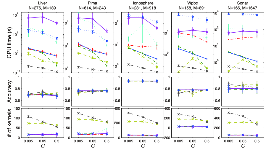
Figure 3: Mean and standard deviation of performance measures for each MKL method for UCI datasets.

In Table 4, a comparison of the average numbers of outer iterations and SVM evaluations on the UCI datasets is reported. The existing methods (HessianMKL, LevelMKL, SimpleMKL, SILP) iterate the update of the kernel weight $\{d_{m}\}_{m=1}^{M}$ and the SVM evaluation of the objective function at the current weight as illustrated in Section 5. We refer to the combination of these two steps as one outer iteration. Since SimpleMKL requires several SVM evaluations during the line search in gradient descent, the number of outer iterations and that of SVM evaluations are different. As for the other methods, both quantities are same. Obviously ElastMKL requires only one outer iteration, thus the result for ElastMKL is not reported in the table. We can see that in all methods the number of outer iterations decreases as the regularization parameter $C$ increases. This is because as the regularization becomes strong, the required number of kernels becomes small and accordingly the intrinsic problem size becomes small. SpicyMKL and HessianMKL require much smaller number of iterations than others. This shows that these methods have fast convergence rate and thus the solution drastically approaches to the optimal one at each iteration. Comparing the CPU time required by SpicyMKL and HessianMKL, SpicyMKL tends to require light computation per iteration especially for large number of kernels while HessianMKL requires QP to derive the update direction that is heavy for large number of kernels.

Table 4: Average number of outer iterations. Average number of SVM evaluations is also shown in the brace for SimpleMKL.

Dataset	$C$	Spicy	Spicy	Simple	Hessian	Level	SILP
		(hinge)	(logit)
	0.005	22.6	20.1	200.3(3770.2)	13.2	171.6	718.8
Liver	0.05	14.1	14.5	222.2(4800.0)	11.8	138.0	517.2
	0.5	6.7	3.3	134.2(2200.5)	9.4	50.1	237.8
	0.005	31.5	21.5	76.2(1488.9)	15.4	290.7	1020.1
Pima	0.05	13.6	13.9	74.9(1511.7)	12.2	197.9	727.1
	0.5	7.9	3.2	24.6( 470.9)	10.2	30.9	258.0
	0.005	38.0	24.6	184.5(2864.1)	11.3	100.9	1810.3
Ionosphere	0.05	18.3	17.1	188.6(2983.1)	10.3	135.6	1580.1
	0.5	7.8	5.4	57.8(1374.4)	14.4	65.5	972.0
	0.005	24.0	24.4	45.4(1014.2)	11.6	61.3	683.6
Wpbc	0.05	13.2	14.4	49.1(1134.7)	10.7	60.8	514.2
	0.5	6.0	2.0	40.9( 964.4)	7.2	55.4	367.0
	0.005	35.2	27.2	158.3(2736.8)	10.3	193.0	4484.6
Sonar	0.05	16.6	16.8	204.8(3535.3)	10.6	194.2	4356.4
	0.5	7.7	4.2	173.3(3511.4)	19.6	154.4	3862.3

In Figure 4(a), we plot the relative duality gaps against CPU time for a single run of SpicyMKL (with logistic loss and block 1-norm regularization), HessianMKL, LevelMKL and SimpleMKL on the ‘Wpbc’ dataset. We can see that the duality gap of SpicyMKL drops rapidly and it is faster than linear. That supports the super-linear convergence of our method. HessianMKL decreases the duality gap quickly because HessianMKL is a second order method. The duality gap of LevelMKL gradually drops in the early stage, but after several steps, the behavior of duality gap becomes unstable. After all, the duality gap of LevelMKL did not drop below $10^{-2}$ in 500 iteration steps. This is because the size of QP required in LevelMKL increases as the algorithm proceeds so that it gets hard to obtain a precise solution. SILP shows fluctuations of the duality gap so that the duality gap does not decrease monotonically. This is because the sequence of the solutions generated by cutting plane method shows oscillation behavior. Figure 4(b) shows the number of active kernels as a function of the CPU time spent by the algorithm. Here we again observe rapid decrease in the number of kernels for SpicyMKL. This reduces huge amount of computation per iteration. We see a relation between the speed of convergence and the number of kernels in SpicyMKL; as the number of kernels decreases, the time spent per iteration becomes small.

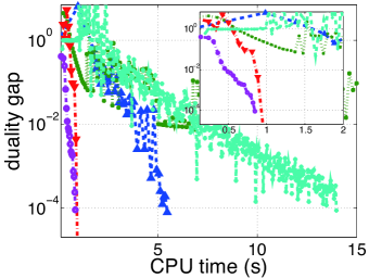
(a) Evolution of Duality Gap

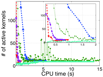
(b) Evolution of # of Active Kernels

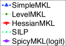
Figure 4: Duality gap and # of active kernels against CPU time

6.2 Scaling against the sample size and the number of kernels

Here we investigate the dependency of CPU time on the number of kernels and the sample size. We used 4 datasets from IDA benchmark repository (Rätsch et al., 2001): ‘Ringnorm’, ‘Splice’, ‘Twonorm’ and ‘Waveform’. The same relative duality gap criterion with tolerance 0.01 was used. We generated a set of basis kernels by randomly selecting subsets of features and applying a Gaussian kernels with random width $\sigma=5\chi^{2}+0.1$, where $\chi^{2}$ is a chi-squared random variable. Here we report ElastMKL with $\lambda=0.1,0.5$ with hinge and logistic loss in addition to SpicyMKL with block 1-norm regularization with hinge and logistic loss, SimpleMKL, HessianMKL, LevelMKL and SILP.

Figure 5 the number of kernels is increased from 50 to 6000. The graph shows the median of CPU times with 25 and 75 percentiles over 10 random train-test splitting where the size of training set was fixed to 200. We observe that for small number of kernels the CPU time of HessianMKL is the fastest among all methods with block 1-norm regularization. However when the number of kernels is greater than 1000, our method SpicyMKL is clearly the fastest among the methods with block 1-norm regularization. In fact, SpicyMKL is roughly 100 times faster than SimpleMKL, HessianMKL and SILP when the number of kernels is 6000. LevelMKL scales almost same as SpicyMKL, but shows unstable performances in Splice dataset. One reason is that LevelMKL shows the oscillation behavior found in Figure 4(a). In particular, the quadratic programming required in LevelMKL often does not converge until the maximum number of iterations available in CPLEX. The scaling property of SILP against the number of kernels is similar to that of SimpleMKL. Those methods do not have as good scaling property as SpicyMKL against the number of kernels. Here again we observe that ElastMKL regularization is even faster than that with block 1-norm regularization, and shows the best performance among all methods.

In Figure 6 the number of training samples is increased from 500 to 3000. The number of kernels is fixed to 20. SILP shows fairly good computational efficiency among the methods with block 1-norm regularization. Comparing the result of Figure 5, while SILP is not fast for a large number of kernels, SILP converges relatively fast for a small number of kernels and scales well against the number of samples. The CPU time of SpicyMKL and ElastMKL is comparable to that of other methods. In particular, ElastMKL shows the best performance in Splice, Twonorm and Waveform.

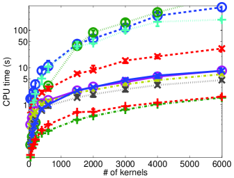
(a) Ringnorm

(b) Splice

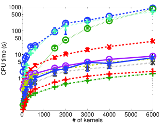
(c) Twonorm

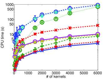
(d) Waveform

Figure 5: CPU time as a function of the number of kernels

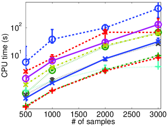
(a) Ringnorm

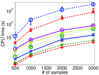
(b) Splice

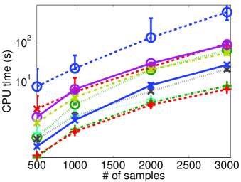
(c) Twonorm

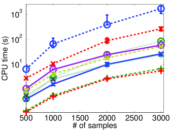
(d) Waveform

Figure 6: CPU time as a function of the sample size

7 Conclusion and future direction

In this article, we have proposed a new efficient training algorithm for MKL with general convex loss functions and general regularizations. The proposed SpicyMKL algorithm generates a sequence of primal variables by iteratively optimizing a sequence of smooth minimization problems. The outer loop of SpicyMKL is a proximal minimization method and it converges super-linearly. The inner minimization is efficiently carried out by the Newton method. We introduced a generalized block norm formulation of MKL regularization that includes non-sparse regularizations such as Elastic-net MKL and block $q$-norm MKL, and derived the connections between our block norm formulation and the kernel weights. Then we derived a general optimization method that is applicable to the general block norm framework. We also gave an efficient one step optimization method for regularizations with smooth dual (e.g., elastic-net and block $q$-norm).

We have shown through numerical experiments that SpicyMKL scales well with increasing number of kernels and it has similar scaling behavior against the number of samples to conventional methods. It is worth noting that SpicyMKL does not rely on solving LP or QP problems, which itself can be a challenging task; accordingly SpicyMKL can reliably obtain a precise solution. SpicyMKL with the logistic loss and elastic-net regularization has shown the best performance while showing fairly good accuracies.

Future work includes a second order modification of the update rule of the primal variables, and combination of the techniques developed in SpicyMKL and wrapper methods (Sonnenburg et al., 2006; Rakotomamonjy et al., 2008; Chapelle and Rakotomamonjy, 2008).

It would also be interesting to develop an efficient decomposition method to deal with a large sample size problem. Since the dual problem (25) of the inner loop is an $N$ dimensional optimization problem, when the number of samples $N$ is large, the naive Newton method or other gradient descent type methods might be hard to be applied. In such a situation, the block-coordinate descent algorithm might be useful. That is, decompose $N$ variables $\{\rho_{i}\}_{i=1}^{N}$ into some groups (say $B$ groups $\{\rho_{I_{i}}\}_{i=1}^{B}$) and iteratively minimize the objective function with respect to one group with other groups fixed:

$$\rho_{I_{i}}^{k+1}\leftarrow\mathop{\arg\min}_{\rho_{I_{i}}}\varphi_{\gamma^{(t)}}((\rho_{I_{1}}^{k+1},\dots,\rho_{I_{i-1}}^{k+1},\rho_{I_{i}},\rho_{I_{i+1}}^{k},\dots,\rho_{I_{B}}^{k});\alpha^{(t)},b^{(t)}).$$

(see Section 5.4.3 of Zangwill (1969) and Proposition 2.7.1 of Bertsekas (1999)). In a similar sense, Sequential Minimal Optimization (SMO) algorithm (Platt, 1999) might be useful for some loss function classes such as the hinge loss. We leave these important issues for future work.

Appendix A Proof of Theorem 1

Combining Eqs. (15), (19), and (24), we can rewrite the dual of the proximal MKL problem (8) as follows:

$$\mathop{\mathrm{minimize}}_{\begin{subarray}{c}\rho\in{\mathbb{R}}^{N}\\ u\in{\mathbb{R}}^{MN}\end{subarray}}\quad\biggl{\{}\textstyle L^{\ast}(-\rho)+\sum\limits_{m=1}^{M}\delta_{C}^{(m)}(u_{m})$$

$$+\sum\limits_{m=1}^{M}\bigl{(}{\alpha_{m}^{(t)}}^{\top}K_{m}(\rho-u_{m})+\frac{\gamma^{(t)}}{2}\|\rho-u_{m}\|_{K_{m}}^{2}\bigr{)}+\!b^{(t)}{\bm{1}}^{\top}\rho\!-\!\frac{\gamma^{(t)}}{2}\!\!\bigl{(}\textstyle{\bm{1}}^{\top}\rho\bigr{)}^{2}\!\biggr{\}},$$

where the maximization is turned into minimization and we redefined $u_{m}/\gamma^{(t)}$ as $u_{m}$. This formulation is known as the augmented Lagrangian for the dual of the MKL optimization problem (7), which can be expressed as follows:

$$\mathop{\mathrm{minimize}}_{\begin{subarray}{c}\rho\in{\mathbb{R}}^{N},\\ u\in{\mathbb{R}}^{MN}\end{subarray}}\quad L^{\ast}(-\rho)+\sum_{m=1}^{M}\delta_{C}^{(m)}(u_{m}),$$

subject to $$K_{m}^{1/2}(\rho-u_{m})=0\quad(m=1,\ldots,M),$$

$$\mathbf{1}^{\top}\rho=0.$$

$K_{m}^{1/2}\alpha_{m}^{(t)}$ and $b^{(t)}$ are the Lagrangian multipliers corresponding to the above $M+1$ equality constraints (Hestenes, 1969; Powell, 1969; Tomioka and Sugiyama, 2009). We apply Proposition 5.11 of Bertsekas (1982) so that we obtain

$$\sum_{m=1}^{M}\|\alpha_{m}^{(t)}-\alpha_{m}^{\ast}\|_{K_{m}}^{2}+(b^{(t)}-b^{\ast})^{2}\to 0~{}~{}~{}~{}(\text{as}~{}t\to\infty).$$

Thus there is sufficiently large $T$ such that for all $t\geq T$, $(\alpha^{(t)},b^{(t)})$ is inside the $\delta$-neighborhood of $(\alpha^{\ast},b^{\ast})$. Therefore we can assume that Eq. (9) holds at $(\alpha^{(t)},b^{(t)})$ for all $t\geq T$. Finally Theorem 3 of Tomioka et al. (2011) (and its proof) gives the assertion (see also the proof of Proposition 5.22 of Bertsekas (1982) where $\phi(t)=t^{2}$ and $\nabla\phi(t)=t$ are substituted for our setting).

References

• Aronszajn (1950) N. Aronszajn. Theory of reproducing kernels. Transactions of the American Mathematical Society, 68:337–404, 1950.
• Asuncion and Newman (2007) A. Asuncion and D. Newman. UCI machine learning repository, 2007. URL http://www.ics.uci.edu/$\sim$mlearn/MLRepository.html.
• Bach (2008) F. R. Bach. Consistency of the group Lasso and multiple kernel learning. Journal of Machine Learning Research, 9:1179–1225, 2008.
• Bach et al. (2004) F. R. Bach, G. Lanckriet, and M. Jordan. Multiple kernel learning, conic duality, and the SMO algorithm. In Proceedings of the 21st International Conference on Machine Learning, pages 41–48, 2004.
• Bach et al. (2005) F. R. Bach, R. Thibaux, and M. I. Jordan. Computing regularization paths for learning multiple kernels. In Advances in Neural Information Processing Systems 17, pages 73–80, Cambridge, MA, 2005. MIT Press.
• Bertsekas (1982) D. P. Bertsekas. Constrained Optimization and Lagrange Multiplier Methods. Academic Press, New York, 1982.
• Bertsekas (1999) D. P. Bertsekas. Nonlinear Programming. Athena Scientific, 1999.
• Candes et al. (2006) E. J. Candes, J. Romberg, and T. Tao. Robust uncertainty principles: Exact signal reconstruction from highly incomplete frequency information. IEEE Transactions on Information Theory, 52(2):489–509, 2006.
• Chapelle and Rakotomamonjy (2008) O. Chapelle and A. Rakotomamonjy. Second order optimization of kernel parameters. In NIPS 2008 Workshop on Kernel Learning: Automatic Selection of Optimal Kernels, Whistler, 2008.
• Cortes (2009) C. Cortes. Can learning kernels help performance? Invited talk at International Conference on Machine Learning (ICML 2009). Montréal, Canada, 2009.
• Cortes et al. (2009) C. Cortes, M. Mohri, and A. Rostamizadeh. $L_{2}$ regularization for learning kernels. In Proceedings of the 25th Conference on Uncertainty in Artificial Intelligence (UAI 2009), 2009. Montréal, Canada.
• Daubechies et al. (2004) I. Daubechies, M. Defrise, and C. D. Mol. An iterative thresholding algorithm for linear inverse problems with a sparsity constraint. Communications on Pure and Applied Mathematics, LVII:1413–1457, 2004.
• Figueiredo and Nowak (2003) M. Figueiredo and R. Nowak. An EM algorithm for wavelet-based image restoration. IEEE Transactions on Image Processing, 12:906–916, 2003.
• Gehler and Nowozin (2009) P. V. Gehler and S. Nowozin. Let the kernel figure it out; principled learning of pre-processing for kernel classifiers. In Proceedings of the IEEE Computer Society Conference on Computer Vision and Pattern (CVPR2009), 2009.
• Hestenes (1969) M. Hestenes. Multiplier and gradient methods. Journal of Optimization Theory & Applications, 4:303–320, 1969.
• Kimeldorf and Wahba (1971) G. S. Kimeldorf and G. Wahba. Some results on Tchebycheffian spline functions. Journal of Mathematical Analysis and Applications, 33:82–95, 1971.
• Kloft et al. (2009) M. Kloft, U. Brefeld, S. Sonnenburg, P. Laskov, K.-R. Müller, and A. Zien. Efficient and accurate $\ell_{p}$-norm multiple kernel learning. In Y. Bengio, D. Schuurmans, J. Lafferty, C. K. I. Williams, and A. Culotta, editors, Advances in Neural Information Processing Systems 22, pages 997–1005, Cambridge, MA, 2009. MIT Press.
• Kloft et al. (2010) M. Kloft, U. Rückert, and P. L. Bartlett. A unifying view of multiple kernel learning, 2010. arXiv:1005.0437.
• Lanckriet et al. (2004) G. Lanckriet, N. Cristianini, L. E. Ghaoui, P. Bartlett, and M. Jordan. Learning the kernel matrix with semi-definite programming. Journal of Machine Learning Research, 5:27–72, 2004.
• Micchelli and Pontil (2005) C. A. Micchelli and M. Pontil. Learning the kernel function via regularization. Journal of Machine Learning Research, 6:1099–1125, 2005.
• Mosci et al. (2008) S. Mosci, M. Santoro, A. Verri, and S. Villa. A new algorithm to learn an optimal kernel based on Fenchel duality. In NIPS 2008 Workshop: Kernel Learning: Automatic Selection of Optimal Kernels, Whistler, 2008.
• Nath et al. (2009) J. S. Nath, G. Dinesh, S. Raman, C. Bhattacharyya, A. Ben-Tal, and K. R. Ramakrishnan. On the algorithmics and applications of a mixed-norm based kernel learning formulation. In Advances in Neural Information Processing Systems 22, pages 844–852, Cambridge, MA, 2009. MIT Press.
• Palmer et al. (2006) J. Palmer, D. Wipf, K. Kreutz-Delgado, and B. Rao. Variational EM algorithms for non-gaussian latent variable models. In Y. Weiss, B. Schölkopf, and J. Platt, editors, Advances in Neural Information Processing Systems 18, pages 1059–1066, Cambridge, MA, 2006. MIT Press.
• Platt (1999) J. C. Platt. Using sparseness and analytic QP to speed training of support vector machines. In Advances in Neural Information Processing Systems 11, pages 557–563. MIT Press, 1999.
• Powell (1969) M. Powell. A method for nonlinear constraints in minimization problems. In R. Fletcher, editor, Optimization, pages 283–298. Academic Press, London, New York, 1969.
• Rakotomamonjy et al. (2008) A. Rakotomamonjy, F. Bach, S. Canu, and G. Y. SimpleMKL. Journal of Machine Learning Research, 9:2491–2521, 2008.
• Rätsch et al. (2001) G. Rätsch, T. Onoda, and K. R. Müller. Soft margins for adaboost. Machine Learning, 42(3):287–320, 2001.
• Rockafellar (1970) R. T. Rockafellar. Convex Analysis. Princeton University Press, Princeton, 1970.
• Rockafellar (1976) R. T. Rockafellar. Augmented Lagrangians and applications of the proximal point algorithm in convex programming. Mathematics of Operations Research, 1:97–116, 1976.
• Schölkopf and Smola (2002) B. Schölkopf and A. J. Smola. Learning with Kernels. MIT Press, Cambridge, MA, 2002.
• Sonnenburg et al. (2006) S. Sonnenburg, G. Rätsch, C. Schäfer, and B. Schölkopf. Large scale multiple kernel learning. Journal of Machine Learning Research, 7:1531–1565, 2006.
• Tomioka and Sugiyama (2009) R. Tomioka and M. Sugiyama. Dual augmented lagrangian method for efficient sparse reconstruction. IEEE Signal Proccesing Letters, 16(12):1067–1070, 2009.
• Tomioka and Suzuki (2009) R. Tomioka and T. Suzuki. Sparsity-accuracy trade-off in MKL, 2009. arXiv:1001.2615.
• Tomioka and Suzuki (2011) R. Tomioka and T. Suzuki. Regularization strategies and empirical bayesian learning for MKL, 2011. arXiv:1011.3090.
• Tomioka et al. (2011) R. Tomioka, T. Suzuki, and M. Sugiyama. Super-linear convergence of dual augmented lagrangian algorithm for sparse learning. Journal of Machine Learning Research, page to appear, 2011.
• Wright et al. (2009) S. J. Wright, R. D. Nowak, and M. A. T. Figueiredo. Sparse reconstruction by separable approximation. IEEE Transactions on Signal Processing, 2009.
• Xu et al. (2009) Z. Xu, R. Jin, I. King, and M. R. Lyu. An extended level method for efficient multiple kernel learning. In Advances in Neural Information Processing Systems 21, pages 1825–1832, Cambridge, MA, 2009. MIT Press.
• Yuan and Lin (2006) M. Yuan and Y. Lin. Model selection and estimation in regression with grouped variables. Journal of The Royal Statistical Society Series B, 68(1):49–67, 2006.
• Zangwill (1969) W. I. Zangwill. Nonlinear Programming: A Unified Approach. Prentice Hall, 1969.
• Zien and Ong (2007) A. Zien and C. Ong. Multiclass multiple kernel learning. In Proceedings of the 24th international conference on machine learning, pages 11910–1198. ACM, 2007.