The cationic energy landscape in alkali silicate glasses: properties and relevance

Heiko Lammert

hlammert@ucsd.edu

Center for Theoretical Biological Physics, University of California San Diego, 9500 Gilman Dr., La Jolla, CA 92093-0374

Radha D. Banhatti

banhatt@uni-muenster.de

Andreas Heuer

andheuer@uni-muenster.de

Institute of Physical Chemistry and Sonderforschungsbereich 458, University of Münster, Corrensstr. 30, D-48149 Münster, Germany

Abstract

Individual cationic site–energies are explicitly determined from molecular dynamics simulations of alkali silicate glasses, and the properties and relevance of this local energetics to ion transport are studied. The absence of relaxations on the timescale of ion transport proves the validity of a static description of the energy landscape, as it is generally used in hopping models. The Coulomb interaction among the cations turns out essential to obtain an average energy landscape in agreement with typical simplified hopping models. Strong correlations exist both between neighboring sites and between different energetic contributions at one site, and they shape essential characteristics of the energy landscape. A model energy landscape with a single vacancy is used to demonstrate why average site–energies, including the full Coulomb interaction, are still insufficient to describe the site population of ions, or their dynamics. This model explains how the relationship between energetics and ion dynamics is weakened, and thus establishes conclusively that a hopping picture with static energies fails to capture all the relevant information. It is therefore suggested that alternative simplified models of ion conduction are needed.

1 Introduction

The transport of mobile modifier ions in silicate glasses below the glass transition takes place in a basically fixed environment provided by the glass structure. Besides the disordered structure of the network, the Coulomb interactions among the mobile ions add significantly to the complexity of the underlying energy landscape, because their contribution is both long–ranged and non–static.

A hopping picture of the dynamics has been widely accepted,¹ based on evidence for the existence of well defined ionic sites, from experiments^{3, 2, 5, 4, 6} and also from simulations^{7, 8, 9}. Basically hopping models describe the glass system by a representation of the effective energy landscape experienced by the ions. The conformational disorder of the network is typically represented by a distribution of site–energies. They are treated as static, relying on the separation of timescales between ion dynamics and structural relaxation.¹⁰ Energy values for individual sites and barriers are normally treated as independent of each other in realizations by lattice models; see, e.g., ¹. This common assumption is however not trivial, and it has been dropped in at least one case.¹¹ Numerical investigations of such simplified models have established that the Coulomb interaction between the mobile ions is required for a completely correct representation of the dynamics,¹² and a quantitative model of the ionic conductivity has been built with the interactions among the ions as the main element.¹³ Most other approaches however disregard the Coulomb interaction among the mobile ions.^{14, 8, 15, 12, 18, 6, 17, 16} This immediately raises the question whether the Coulomb interaction can be simply taken into account by a local modification of the energy landscape.

Recently a statistical method allowed us the identification of all ionic sites in realistic molecular dynamics $(\mbox{MD})$ simulations.¹⁹ Most of the conclusions have been confirmed by other groups. ^{21, 20}. By direct observation of the ion hopping dynamics, key predictions about the ion dynamics could be tested.²². Furthermore, different spatial aspects of the conduction paths have been reported ^{26, 27, 25, 23, 24}.

Most of the hopping models mentioned above use the concept of site–energies. However, typically the properties of these site–energies are postulated in an ad-hoc manner. In the present work we express the properties of the energy landscape via explicitly determined site-energies. These are obtained based on our $(\mbox{MD})$ simulations of alkali silicate systems, from time-averages of the particle energy of the ion residing in a site. Two key questions are addressed: What are the properties of the site–energies for a real ion conductor? Do these site–energies indeed determine thermodynamic or dynamic properties of the corresponding sites? In particular, since the Coulomb interaction between cations can be expected to be strong, it is not evident a priori that it can be taken into account as merely a contribution to single-particle or, equivalently, single–site energies. This aspect is discussed in detail by examining the correlation of site–energies to thermodynamical and dynamical observables.

2 Method

In our MD simulations the potential energy is given by pair interactions as $U_{\mathrm{sys}}=1/2\sum_{i,j\neq{}i}U_{ij}$. The interaction potential $U_{ij}(r_{ij})=q_{i}q_{j}/(4\pi\varepsilon_{0}r_{ij})-A_{ij}r_{ij}^{-6}+B_{ij}\exp(-C_{ij}r_{ij})$ consists of the Coulomb interaction for point charges $U^{\mathrm{Q}}_{ij}$ and of a short range part $U^{\mathrm{BM}}_{ij}$ of Born-Mayer type. The $q_{i,j}$ reflect appropriately chosen partial charges ⁸.

For a finite system, single-particle energies $U_{i}$ can be computed just like $U_{\mathrm{sys}}$ as the sum of all pair contributions $U_{ij}$ involving the particle $i$, $U_{i}=\sum_{j\neq i}U_{ij}$. While $\sum_{i}U_{i}=2U_{\mathrm{sys}}$, any change $\Delta U_{\mathrm{sys}}$ to the energy of the system resulting from a change of particle $i$ is directly given by $\Delta U_{i}$. Considering a cation as particle $i$, the contribution to $U_{i}$ only from interactions with e.g. other cations can furthermore be isolated simply by restricting the sum to the appropriate $j$.

The situation is complicated by the use of periodic boundary conditions: To avoid finite-size effects, the system is treated as an infinite repetition of periodic images of the simulation box.²⁸ Due to the long range nature of the Coulomb interaction, it cannot be computed by simple summation up to a finite cutoff in this case. Instead all periodic images of the simulation box must be taken into account. We use the Ewald method²⁸ for this purpose, where the Coulomb energy is broken into three formal contributions: Only the real part $U^{\mathrm{RE}}_{ij}$ is a pair term like $U^{\mathrm{BM}}_{ij}$; the Fourier part $U^{\mathrm{FO}}_{ij}$ relates to the infinite set of periodic images of particle $j$, and the self-correction $U^{\mathrm{SE}}_{i}$ is globally assigned to particle $i$ only.

Yet a deeper analysis shows that the Coulomb part $U^{\mathrm{Q}}_{i}$ of a single-particle energy can still be assembled from these terms, and that it can still be divided into contributions from groups of like particles. One can notably still separate the interaction of a cation with other cations $U^{\mathrm{cat}}_{i}$ from the interaction with network atoms $U^{\mathrm{net}}_{i}$, because $U^{\mathrm{SE}}_{i}$ can be traced exclusively to the cation part. A constant correction²⁹ for the nonzero charge of the partial systems under consideration is neglected, because it does not affect the results of this study, where energy differences are relevant.

As the locations and structural properties of the sites are stable on the time scale of alkali ion diffusion, the potential energy of cation $i$ is determined by the site $s(i)$ it occupies. A site–energy $E(s)$ can therefore be identified by taking the time average over the particle energy of the ions $i(s,t)$ residing in $s$ at any given time $t$, i.e. $E(s)=\left<U_{i(s,t)}(t)\right>_{t}$. Like the particle energies, the total value of the site–energy $E^{\mathrm{tot}}(s)$ is separated into the contributions $E^{\mathrm{cat}}(s)$ and $E^{\mathrm{net}}(s)$. Of course, with this construction $E(s)$ cannot be interpreted as a bare site–energy but reflects the site–energy under the condition that it is populated by an ion.

3 Systems

We analyzed the site–energies for the alkali disilicate systems $(\mathrm{Li}_{2}\mathrm{O})\cdot 2(\mathrm{SiO}_{2})$ and $(\mathrm{K}_{2}\mathrm{O})\cdot 2(\mathrm{SiO}_{2})$, named $\mathrm{LS\!\!-\!\!2}$ and $\mathrm{KS\!\!-\!\!2}$ respectively. These systems have already been described in our previous work²². They contain 270 cations among 1215 atoms, at experimental densities³⁰. Interactions are given by a potential by Habasaki et al.³¹. The systems were propagated with a timestep of 2 $\>{\rm fs}$ in the canonical ensemble, using a Nosé-Hoover thermostat³². Positions and energy contributions were stored every 0.1 $\>{\rm ps}$, with energies averaged over five values sampled 20 $\>{\rm fs}$ apart. Energy data was produced for 10 $\>{\rm ns}$ of simulations at 850 $\>{\rm K}$.

Our analysis identifies for these datasets 291 and 276 sites respectively in $\mathrm{LS\!\!-\!\!2}$ and $\mathrm{KS\!\!-\!\!2}$. Ions are in all cases residing in a site during more than $98\%$ of the times, according to our algorithm that drops excursions.¹⁹

4 Results

4.1 Properties of average site–energies

It turns out that the fundamental characteristics of the energy landscape are qualitatively identical in both systems. Note that these energies result from long time averages. Possible temporal fluctuations are discussed further below. Broad ranges of site–energies reflect the variation in the disordered structure. For $E^{\mathrm{tot}}$ the distributions can be fitted by Gaussians, with the parameters given in Tab. I. The properties of the distributions are compatible with earlier results, determined both for sites²⁰, and without reference to ion sites^{33, 34, 9, 35}.

System	$\mu[\>e\mathrm{V}]$	$\sigma_{dist}[\>e\mathrm{V}]$
$\mathrm{LS\!\!-\!\!2}$	-8.8	0.33
$\mathrm{KS\!\!-\!\!2}$	-5.6	0.24

Table I: Gaussian fits for the distribution of site energies $f(E^{\mathrm{tot}})$

The influence of interactions with both cations and network on the shape of the site–energy distributions is demonstrated in Fig. 1 for the system $\mathrm{LS\!\!-\!\!2}$. For each site the cation contribution $E^{\mathrm{cat}}(s)$ is plotted against the corresponding network energy $E^{\mathrm{net}}(s)$. Both sets of energies have standard deviations of 5 to 6 $\>e\mathrm{V}$ and cover ranges of more than 20 $\>e\mathrm{V}$. In the system $\mathrm{KS\!\!-\!\!2}$ standard deviations of 3 $\>e\mathrm{V}$ and ranges of 16 $\>e\mathrm{V}$ are found. In all cases the significantly narrower distributions for $E^{\mathrm{tot}}(s)$ are reached because a strong and clear anticorrelation between $E^{\mathrm{cat}}(s)$ and $E^{\mathrm{net}}(s)$, evident in Fig. 1, reduces the spread of values for the resulting total site–energies.

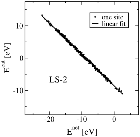
Figure 1: Contributions $E^{\mathrm{cat}}(s)$ and $E^{\mathrm{net}}(s)$ for each site $s$ in system $\mathrm{LS\!\!-\!\!2}$

Naturally, the strong variation of $E^{\mathrm{net}}$ can be interpreted as a consequence of the disordered network structure. The presence of non-bridging oxygens (NBO) gives rise to a negative partial charge. Thus, due to the strong Coulomb interaction, a minor variation in the distance between the site and the nearest NBO may result in a significant variation of the network energy. The typical distance between a $\mathrm{Li}$-ion and a NBO is 2Å. For example, variation of this distance by 0.1Å gives rise to an energy variation of $\pm 0.4\>e\mathrm{V}{}$, for the potential used in these simulations.

To test the assumption of many lattice models that the site–energies are uncorrelated, the energies of all sites were compared to those of their next neighbors, defined by the first nearest-neighbor shell of the alkali pair distribution. The results are shown in Fig. 2 for the glass $\mathrm{LS\!\!-\!\!2}$, whose behavior is again typical for all investigated systems. For each site $s$ the average energy of the neighbors of $s$ is plotted against the site–energy of $s$ itself. Data for the contribution $E^{\mathrm{net}}$ of the matrix alone is given by the open circles. They show a strong spatial correlation of the network energies between adjacent sites. The same correlation is found for the cation interactions $E^{\mathrm{cat}}$, as it may be expected when $E^{\mathrm{cat}}$ and $E^{\mathrm{net}}$ are anticorrelated themselves. The total energies are shown as squares in the inset. For them spatial correlations are much weaker (regression coefficient 0.26 $\pm$ 0.1), because the remaining imperfections in the cancelation of $E^{\mathrm{cat}}$ and $E^{\mathrm{net}}$ introduce sufficient fluctuations into $E^{\mathrm{tot}}$ to create a nearly uncorrelated disordered landscape.

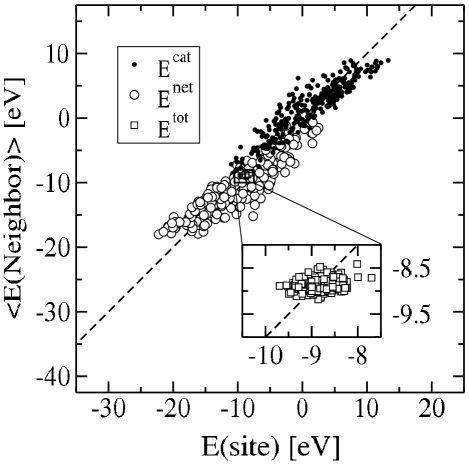
Figure 2: Correlation among the energies of neighboring sites in system $\mathrm{LS\!\!-\!\!2}$

4.2 Temporal variations of site–energies

Temporal variations of site–energies can occur as a consequence of different physical effects: (1) Gradual structural relaxation of the silicate glass, (2) Fluctuations due to motion of adjacent ions. Both aspects are analyzed in this part.

The long-time variation of $E(s)$, resulting from the structural relaxation, was estimated by comparing the mean energy values for each site from the first and from the second half of the available $10\>{\rm ns}$ of data. Judging from the width of the Gaussian distribution of these energy differences, the residual long-time fluctuations of a site–energy $E^{\mathrm{tot}}_{\mathrm{Li}}$ are $0.03\>e\mathrm{V}$ and $0.02\>e\mathrm{V}$ for the Lithium and Potassium glasses. These fluctuations, related to systematic drifts are small as compared to the overall width of the Gaussian distributions; see Tab. I.

As mentioned above the energy value for a single site results from an average over the whole simulation run. Random fluctuations in this site-energy can be observed by defining the energy value instead from very short averages. Two time scales have to be compared. First, the time scale $\tau_{fluct}$ characterizes the time where typical energy fluctuations of a site are explored. Second, $\tau_{res}$ describes typical residence times of an ion in a site. The distribution of $\tau_{res}$ has a median of a few hundred picoseconds (see below). Only if $\tau_{fluct}\ll\tau_{res}$ it is justified to characterize the properties of a site, as experienced by an ion, via the average $E(s)$. In the opposite limit one would have to introduce a time–dependent energy $E(s)$.

In order to check how stable and distinguishable the individual site–energies are, we plot in Fig. 3 the average growth of the standard deviation $\sigma_{E}(t)$ for the set of energy values that are incorporated into the mean site–energy. The variable $t$ denotes the width of the interval, used for calculating the average. The development of the total energy $E^{\mathrm{tot}}$ is shown in the upper part, the lower part treats the network contribution $E^{\mathrm{net}}$. The cation part $E^{\mathrm{cat}}$ is omitted, because its behavior is very similar to that of $E^{\mathrm{net}}$, due to the correlation demonstrated above.

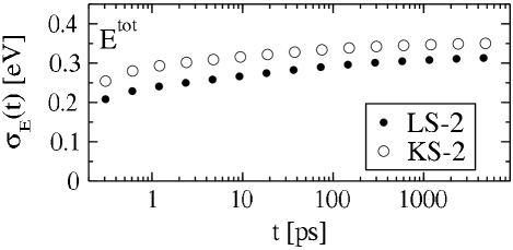
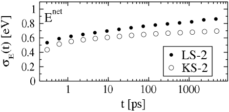
Figure 3: Growth of the standard deviation $\sigma_{E}$ of energies for a site with sampling time. The behavior of $E^{\mathrm{cat}}$ is similar to that for $E^{\mathrm{net}}$.

First, it turns out that for $\mathrm{LS\!\!-\!\!2}$ beyond 100 ps a nearly constant value of $\sigma_{E}(t)$ is observed. Thus, indeed, the typical fluctuation time $\tau_{fluct}$ is much shorter than $\tau_{res}$. The range of values sampled for the energy of a typical site has a considerable width. It reaches a value of $\sigma(t=4.6\>{\rm ns})=0.31\>e\mathrm{V}$ at the end of the plot for $E^{\mathrm{tot}}_{\mathrm{Li}}$ in $\mathrm{LS\!\!-\!\!2}$, and of $\sigma(t=4.6\>{\rm ns})=0.35\>e\mathrm{V}$ for $E^{\mathrm{tot}}_{\mathrm{K}}$ in $\mathrm{KS\!\!-\!\!2}$. The overall stability of the energies on a timescale of more than 5 $\>{\rm ns}$ is supported by the small errors for $E^{\mathrm{tot}}$ determined above.

The site–energies, introduced so far, provide an average view of the energy landscape, as it is adopted by most hopping models. In principle one might envisage a scenario where dynamical events induce systematic changes in the local configuration. Specifically the energy of a site might change as a consequence of an ionic jump. For example, in the MIGRATION concept ¹³ an ion, jumping to a site, is thought to be gradually stabilized by the subsequent adaption of the other ions to that jump. In this scenario one might expect a gradual decrease of the site–energy via a decrease of $E^{\mathrm{cat}}$. Of course, for reasons of time-reversal symmetry it has to increase correspondingly before the jump to the next site.

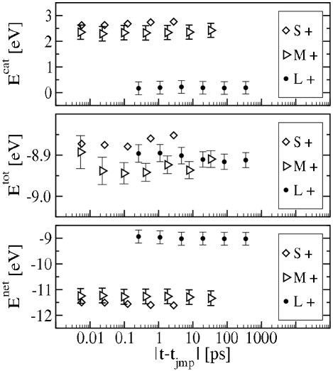
Figure 4: Development of the energy of an ion directly after the jump into a site, at $t=t_{\mathrm{jmp}}$. Three sets of residences with different duration are distinguished, designated Short, Medium and Long. Behavior at the end of a residence before the jump is equivalent.

To analyse a possible time-dependence we recorded the time-dependence of the energy during residences by the ions. Here we restrict ourselves to the system $\mathrm{LS\!\!-\!\!2}$. A possible time-dependence would naturally depend on the typical residence time of an ion in a site. Therefore, we have grouped the different residence times into bins, namely S: $\tau\in[10\>{\rm ps}{},100\>{\rm ps}{}]$, M: $\tau\in[100\>{\rm ps}{},1\>{\rm ns}{}]$, and L: $\tau\in[1\>{\rm ns}{},10\>{\rm ns}{}]$. The results are shown in Fig. 4. For groups S and M we performed additional simulations with a sampling interval of 2 $\>{\rm fs}$ (during 1 ns). For group L the data from our main simulations is shown, with a sampling interval of 100 $\>{\rm fs}$. Plotted times extend up to 10 % of the maximum duration, such that values are available from all residences in the group.

The time dependencies of the energies from the start and from the end of the residence were both investigated. The positive direction of time was defined in both cases away from the nearest jump, such that the plotted time increases always towards the middle of the residence. Only the development from the start of the residences is shown here. In all cases the data from the end of the residences is identical within the errors, given by either error bars or symbol size.

It is clearly seen that, if at all, $E^{\mathrm{cat}}$ and $E^{\mathrm{net}}$ slightly change with time for the shortest residences. After their addition to the total energy $E^{\mathrm{tot}}$ only unsystematic fluctuations remain. In conclusion no energetic relaxations are observed when an ion reaches a site, or before it leaves. The average site–energies are therefore the appropriate quantities for a deeper analysis of the behavior of the systems.

4.3 Site–energy vs. thermodynamics

The residence times are linked to the site–energies in an indirect way, via the height of the energy barrier between two sites. While it is probably not crucial, this complication is absent for the thermodynamic occupation probabilities of the sites, which should depend directly on their energies via a Fermi distribution.

In Fig. 5 this prediction is tested for the system $\mathrm{LS\!\!-\!\!2}$. A Fermi function with $\mu=-8.4\>e\mathrm{V}{}$ is given by the solid line. The value of $\mu$ was chosen such that the predicted total occupation of all sites from the MD simulation corresponds to the number of alkali ions. However the occupation data for the individual sites from the MD simulation, given by the solid circles, deviate fundamentally from a Fermi function. No clear dependence of the relative occupation on the site–energy can be observed. For comparison, a system with the same number of sites and ions and with the site–energies $E^{\mathrm{tot}}$ found in the MD system was propagated in a Monte Carlo simulation. The occupation data from this simulation, given by the open circles, nicely agrees with the theoretical Fermi function.

Some minor deviations in the MD data might occur from the fact that in disagreement with the derivation of the Fermi relationship³⁶ many sites may very rarely host two ions at the same time. However, as seen from Fig. 5 only 4 sites have an average number of hosted ions which is significantly larger than unity. Therefore this effect cannot be responsible for the significant deviations.

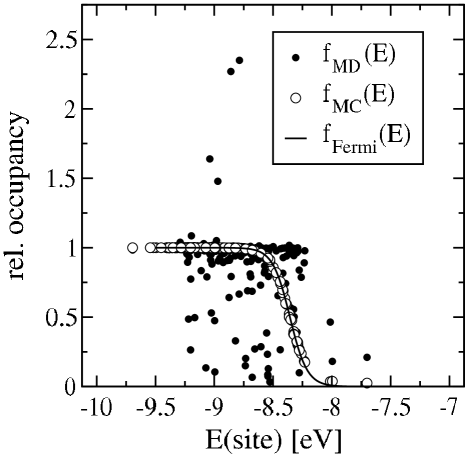
Figure 5: Mean relative occupation of the sites in $\mathrm{LS\!\!-\!\!2}$ plotted against $E^{\mathrm{tot}}$. The solid line is a Fermi-Dirac function with $\mu=8.4\>e\mathrm{V}{}$, the open symbols were generated from a Monte Carlo model that recreates the MD system (see text).

4.4 Site–energy vs. dynamics

Another interesting observation in Fig.4 is the correlation of $E^{\mathrm{cat}}$ and $E^{\mathrm{net}}$ with the residence time. For long residences, represented by $L$, $E^{\mathrm{cat}}$ is smaller whereas $E^{\mathrm{net}}$ displays the opposite trend. The data in Fig. 4 also suggest that a minor correlation along this line seems to remain for $E^{\mathrm{tot}}$. Sites with short residence times have somewhat higher total energies $E^{\mathrm{tot}}$. This has been systematically analyzed in Fig. 6 for the system $\mathrm{LS\!\!-\!\!2}$. For each site the mean residence time $\tau_{\mathrm{res}}$for ions in a site is plotted against the network energy $E^{\mathrm{net}}$ and against the site–energy $E^{\mathrm{tot}}$.

On average there is some increase of the residence time with increasing network energy. As directly indicated by the major scatter the correlation coefficient between $\log\tau_{\mathrm{res}}$ and $E^{\mathrm{net}}$ is relatively small (0.28). The dependence of $\log\tau_{\mathrm{res}}$ on $E^{\mathrm{tot}}$ is also present, but shows an even weaker correlation coefficient.(-0.18) A possible reason for these weak correlations is discussed below.

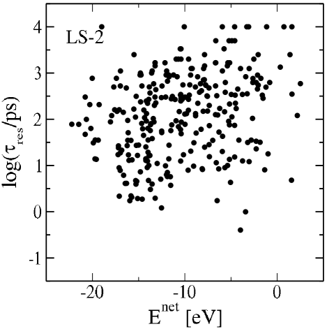
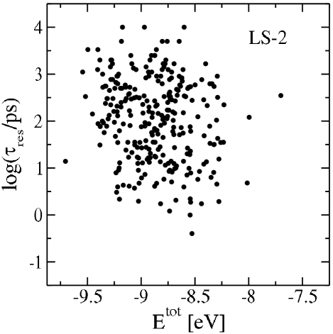
Figure 6: Mean residence times $\tau_{\mathrm{res}}$ plotted against the site–energies $E^{\mathrm{net}}$ and $E^{\mathrm{tot}}$.

5 Model energy landscape

The deviations of ion behavior from expectations based on the average energies, like the Fermi distribution for relative occupations, can be understood when considering the effect of ion-ion interactions. To visualize this effect we use a very simple model with $N$ sites and $N-1$ ions. This choice reflects the observed small number of free sites. Let $E^{\mathrm{net}}(s)$ denote the energy of an ion at site $s$ due to the interaction with the network. Furthermore, $E^{\mathrm{vac},t}(s)$ denotes the additional energy of an ion at site $s$ due to the interaction with the other ions under the condition that site $t$ ($t\neq s$) is empty. One expects a small but significant dependence of $E^{\mathrm{vac},t}(s)$ on $t$, e.g., via the distance of site $t$ to site $s$. Furthermore, this term also contains possible correction effects of the network energy because the network structure may also depend on the actual ionic configuration. The energy $E^{\mathrm{vac,total}}(t)=\sum_{s\neq t}[E^{\mathrm{net}}(s)+E^{\mathrm{vac},t}(s)]$ thus denotes the total energy of the system under the condition that site $t$ is vacant. Correspondingly, the equilibrium probability $p^{\mathrm{vac},t}$ that site $t$ is empty is proportional to $\exp(-\beta E^{\mathrm{vac,total}}(t))$.

For this model one can first calculate the average energy $E^{\mathrm{tot}}(s)$ related to site $s$. It is given by

$$E^{\mathrm{tot}}(s)=E^{\mathrm{net}}(s)+\frac{\sum_{t=1;t\neq s}^{N}E^{\mathrm{vac},t}(s)p^{\mathrm{vac},t}}{1-p^{\mathrm{vac},s}}.$$ (1)

Via the Boltzmann average this expression implies that the typical residence time is longer than the typical energy fluctuations via jumps of surrounding particles. This ansatz is compatible with the simulation results because the fluctuations of the energy are much faster than typical residence times ($\tau_{fluc}\ll\tau_{res}$. The probability that site $s$ is occupied by an ion can be calculated as

$$p^{\mathrm{ion}}(s)=1-p^{\mathrm{vac},s}.$$ (2)

In Fig. 7 $p^{\mathrm{ion}}(s)$ is compared to the Fermi distribution, based on the average site–energy $E^{\mathrm{tot}}(s)$ for the case that $E^{\mathrm{net}}(s)$ is drawn from a box distribution $[0,4k_{B}T]$. Without the additional contribution of $E^{\mathrm{vac},t}(s)$ the Fermi distribution is indeed very well reproduced. Actually, for just a single vacancy the Fermi distribution is only an approximation but the difference to the true distribution is small. The situation dramatically changes when the additional contributions $E^{\mathrm{vac},t}(s)$ are taken into account. They are considered as random numbers, drawn from a narrower box distribution $[0,0.5k_{B}T]$. One can clearly see that now significant deviations from the Fermi distribution are observed. Thus, even a small interaction among the ions significantly invalidates the applicability of the Fermi distribution and renders averaged total site–energies unsuitable for the prediction of the population of that site.

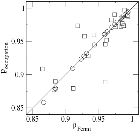
Figure 7: Comparison of the probability $p^{\mathrm{ion}}(s)$ for the ion population of site $s$ in a simple vacancy model (see text) with its Fermi estimate. In one case (circles) the ion-ion interaction does not depend on the position of the vacancy, in the other case (squares) a weak dependence has been taken into account (see text for details).

6 Discussion

The site–energies that are the basis for this investigation of the energy landscape for ionic transport can be determined with good precision as averages from long molecular dynamics simulations. While there are fast fluctuations, the mean value of the site–energy is stable on the timescale of the typical residence of alkali ions in a site. The observed stability of the site–energies and the absence of relevant relaxations on longer time scales, i.e. on the scale of ionic diffusion or beyond, are necessary conditions for our analysis.

A description of the energy landscape through a distribution of static site–energies, as it is used in most hopping models, is well justified by these results. Our analysis demonstrates that fundamental properties of the energy landscape assumed by these models depend on the Coulomb interaction among the cations. Strong correlations in the network energies of neighbor sites are canceled out by the cation interaction to yield a nearly random landscape. Both the spatial correlations in $E^{\mathrm{net}}$ and its anticorrelation with $E^{\mathrm{cat}}$ are reproduced by the counter ion model³⁷ by using full Coulomb interactions between mobile cations and fixed anions on a lattice. Arguably, any realistic energy landscape for a hopping model must at least implicitly incorporate effects of the cation interaction. One further example is the introduction of spatial correlations into the energy landscape of a model designed to reproduce the internal friction of mixed–alkali glasses.¹¹

Both observed correlations in the landscape can be tentatively explained by an argument similar to that used by Greaves in favor of conduction channels.² He stated that any non–bridging oxygen (NBO) in the structure has to be shared between several cations in order to fulfill all coordination requirements. Aided by the long range of the Coulomb interaction, the presence of an NBO can thus influence the energies of several neighboring sites alike. Higher numbers of available NBOs will similarly favor not a single site, but a region of the system. But such a region will be energetically favorable to the cations only just until their mutual repulsion balances the effect of the structure, giving rise to the observed anticorrelation.

The correlations between neighboring sites and between the different contributions at one site are in turn essential for features of the landscape that directly affect the dynamics. While barrier heights for jumps between sites were not determined, the difference between two site–energies gives a lower bound for the barrier for the transition between them. Although the correlations in $E^{\mathrm{net}}$ limit the occurring differences, the additional smoothing of the landscape by the anticorrelated $E^{\mathrm{cat}}$ is necessary to reach values as small as 0.33 eV for $\mathrm{LS\!\!-\!\!2}$. Interestingly, this value is significantly smaller than the macroscopic activation energy of 0.66 eV. Two reasons may play a role. One may expect that the barriers between the sites also make a significant contribution to the macroscopic activation energy. Moreover we have seen that the local dynamics is only weakly correlated with the local energy.

In Fig. 6 the correlations between site–energies and residence times are obscured by scatter that dominates the results for most sites. The larger values of $E^{\mathrm{net}}$ observed for slow sites suggest a low density of non-bridging oxygen (NBOs) atoms and, correspondingly, a high density of bridging oxygen (BOs) nearby. This is fully compatible with the previous observation that sites with long residence times are surrounded by a larger number of BOs³⁸. The physical reason is that the jump process of an ion is supplemented by an instantaneous local door-opening effect of oxygen atoms ^{40, 39}. In case where the neighborhood contains BOs the door-opening effect is reduced, giving rise to a longer residence time. This structural trend is however only sufficient to indicate very slow sites, just as the network energies support only a general relationship, but no clear prediction of the dynamics at any individual site. The even weaker dependence of the residence times on $E^{\mathrm{tot}}$ indicates that the average site energies do not capture all effects of the added cation interaction on the local dynamics.

But also considering equilibrium properties the full site–energies, with the cation interaction included, have still proven insufficient to determine the behavior of ions at the individual sites. The most fundamental test for the importance of the site–energies in our systems is shown in Fig. 5, where the influence of the site–energies on their occupation probability is investigated. The relative occupation of the sites deviates fundamentally from the expected Fermi dependence. These observations clearly indicate that average single–site–energies, as defined here (thus, taking into account the long-range interaction) and used in many of the models of ion conduction, do not contain the complete information.

The simple model analyzed in Fig. 7 suggests the reason: Coupling of the site–energies to other, distant parts of the system makes states of identical local occupation energetically non-equivalent. In consequence the statistics yielding e.g. the Fermi distribution are disrupted. In the glass simulated by the MD model, the fluctuations of the site–energy are fast compared to the duration of a residence. But for the case of only a few unoccupied sites the relaxation rate also strongly depends on the availability of free nearby sites. As jumps happen with delays much shorter than the total residence times once a free site is available, the effective timescale on which the site–energy acts on the occupation becomes comparable to the timescale of fast energy fluctuations. As a consequence only a weak correlation between residence time and site–energy is to be expected.

7 Conclusions

We have shown that it is possible to describe the energy landscape for ion conduction in a glass in terms of stable average site–energies. The analysis of site–energies has established a central influence of the cation interaction on the basic properties of the energy landscape. Yet average site–energies including cation interactions are still insufficient to predict the ion dynamics directly. The dependence of the site–energies on the ionic configuration, and the low number of free sites, which regulates the possibility for jumps independently from the energies, are demonstrated as the likely causes.

A direct description of the dynamics starting from site–energies will therefore not be able to capture the correlations among the ions. Instead the falsification of the single–energy picture suggests that alternative ways should be explored to build a description of the ion dynamics from information about the energy landscape.

In particular a treatment in terms of vacancies seems promising^{41, 19, 42} because due to their small concentration interaction effects can be expected to be negligible. They offer an equivalent description of the ion dynamics, without loss of microscopic detail, because every jump of an ion can be replaced by a corresponding jump of a vacancy. Work along this line will be published elsewhere.

References

- 1 S. D. Baranovskii and H. Cordes, J. Chem. Phys. 111, 7546 (1999).
- 2 G. N. Greaves, J. Non-Cryst. Solids 71, 203 (1985).
- 3 G. N. Greaves, A. Fontaine, P. Lagarde, D. Raoux, and S. J. Gurman, Nature 293, 611 (1981).
- 4 N. Kamijo, K. Handa, and N. Umesaki, Materials Transactions, JIM 37, 927 (1996).
- 5 G. B. Rouse, P. J. Miller, and W. M. Risen, J. Non-Cryst. Solids 28, 193 (1978).
- 6 J. Swenson et al., Phys. Rev. B 63, art. no. 132202 (2001).
- 7 S. Balasubramanian and K. J. Rao, J. Phys. Chem. 97, 8835 (1993).
- 8 J. Habasaki, I. Okada, and Y. Hiwatari, J. Non-Cryst. Solids 183, 12 (1995).
- 9 B. Park and A. N. Cormack, J. Non-Cryst. Solids 255, 112 (1999).
- 10 C. A. Angell, Solid State Ion. 9–10, 3 (1983).
- 11 R. Peibst, S. Schott, and P. Maass, Phys. Rev. Lett. 95, 115901 (2005).
- 12 P. Maass, J. Non-Cryst. Solids 255, 35 (1999).
- 13 K. Funke and R. D. Banhatti, Solid State Ionics 169, 1 (2004).
- 14 A. Bunde, M. D. Ingram, P. Maass, and other, J. Phys. A: Math. Gen. 24, L881 (1991).
- 15 A. G. Hunt, J. Non-Cryst. Solids 220, 1 (1997).
- 16 A. W. Imre, S. V. Divinski, S. Voss, F. Berkemeier, and H. Mehrer, Journal Of Non-Crystalline Solids 352, 783 (2006).
- 17 M. D. Ingram, C. T. Imrie, and I. Konidakis, Journal Of Non-Crystalline Solids 352, 3200 (2006).
- 18 R. Kirchheim and D. Paulmann, J. Non-Cryst. Solids 286, 210 (2001).
- 19 H. Lammert, M. Kunow, and A. Heuer, Phys. Rev. Lett. 90, 215901 (2003).
- 20 J. Habasaki and Y. Hiwatari, Phys. Rev. B 69, 144207 (2004).
- 21 M. Vogel, Phys. Rev. B 70, 094302 (2004).
- 22 H. Lammert and A. Heuer, Phys. Rev. B 72, 214202 (2005).
- 23 S. Adams and J. Swenson, Phys. Chem. Chem. Phys 4, 3179 (2002).
- 24 J. Habasaki and K. L. Ngai, Physical Chemistry Chemical Physics 9, 4673 (2007).
- 25 J. Horbach, W. Kob, and K. Binder, Phys. Rev. Lett. 88, 125502 (2002).
- 26 P. Jund, W. Kob, and R. Jullien, Phys. Rev. B 64, 134303 (2001).
- 27 A. Meyer, H. Schober, and D. B. Dingwell, Europhys. Lett. 59, 708 (2002).
- 28 D. Frenkel and B. Smit, Understanding Molecular Simulations, Academic Press, 2nd edition, 2002.
- 29 F. Figueirido, G. D. Del Buono, and R. M. Levy, J. Chem. Phys. 103, 6133 (1995).
- 30 N. P. Bansal and R. H. Doremus, Handbook of Glass Properties, Academic Press, Orlando, 1986.
- 31 J. Habasaki and I. Okada, Molec. Simul. 9, 319 (1992).
- 32 W. G. Hoover, Phys. Rev. A 31, 1695 (1985).
- 33 S. Balasubramanian and K. J. Rao, J. Non-Cryst. Solids 181, 157 (1995).
- 34 J. Habasaki, I. Okada, and Y. Hiwatari, J. Non-Cryst. Solids 208, 181 (1996).
- 35 E. Sunyer, P. Jund, and R. Jullien, Phys. Rev. B 65, 214203 (2002).
- 36 A. A. Gusev and U. W. Suter, Phys. Rev. A 43, 6488 (1991).
- 37 D. Knödler, P. Pendzig, and W. Dieterich, Solid State Ionics 86–88, 29 (1996).
- 38 H. Lammert and A. Heuer, Phys. Rev. B 70, 024204 (2004).
- 39 M. Kunow and A. Heuer, Phys. Chem. Chem. Phys 7, 2131 (2005).
- 40 E. Sunyer, P. Jund, and R. Jullien, J. Phys.: Condens. Matter 15, L431 (2003).
- 41 A. N. Cormack, J. Du, and T. R. Zeitler, Phys. Chem. Chem. Phys. 4, 3193 (2002).
- 42 J. C. Dyre, J. Non-Cryst. Solids 324, 192 (2003).