Magnetic order and dynamics of the charge-ordered antiferromagnet La_1.5Sr_0.5CoO₄

Abstract

We describe neutron scattering experiments performed to investigate the magnetic order and dynamics of half-doped La_1.5Sr_0.5CoO₄. This layered perovskite exhibits a near-ideal checkerboard pattern of Co²⁺/Co³⁺ charge order at temperatures below $\sim 800$ K. Magnetic correlations are observed at temperatures below $\sim 60$ K but static magnetic order only becomes established at $31$ K, a temperature at which a kink is observed in the susceptibility. On warming above $31$ K we observed a change in the magnetic correlations which we attribute either to a spin canting or to a change in the proportion of inequivalent magnetic domains. The magnetic excitation spectrum is dominated by an intense band extending above a gap of approximately 3 meV up to a maximum energy of 16 meV. A weaker band exists in the energy range 20–30 meV. We show that the excitation spectrum is in excellent quantitative agreement with the predictions of a spin-wave theory generalized to include the full magnetic degrees of freedom of high-spin Co²⁺ ions in an axially distorted crystal field, coupled by Heisenberg exchange interactions. The magnetic order is found to be stabilized by dominant antiferromagnetic Co²⁺–Co²⁺ interactions acting in a straight line through Co³⁺. No evidence is found for magnetic scattering from the Co³⁺ ions, supporting the view that Co³⁺ is in the $S=0$ state in this material.

I Introduction

Hole-doped transition-metal oxide antiferromagnets exhibit a range of intriguing phenomena, including unconventional superconductivity, metal–insulator transitions, magnetoelectric behavior and extreme sensitivity to external stimuli. Their more unusual properties are often found in association with electronically-ordered states with nano-scale periodicity arising from competition between electronic, magnetic and structural degrees of freedom. As well as being of fundamental interest, these highly correlated phases offer the possibility to tune the macroscopic properties of a material via selective control of its microscopic states.

At low doping levels, holes introduced into layered antiferromagnet insulators have a tendency to segregate into stripes, as observed for example in layered cupratesTranquada-Nature-1995 , nickelatesChen-PRL-1993 ; Tranquada-PRL-1994 ; Yamada-PhysicaC-1994 and, most recently, in layered cobaltatesCwik-PRL-2009 . Stripes are a form of complex electronic order in which the antiferromagnetic structure is modulated by periodic arrays of hole-rich antiphase boundaries. With increasing doping, stripe-ordered systems can evolve into metallic or charge-ordered insulating states depending on the relative importance of the electron kinetic energy, Coulomb interactions and associated lattice strain.

At half doping, many transition-metal oxides exhibit an insulating charge-ordered phase, the stability of which is generally assisted by cooperative Jahn–Teller distortions. For layered systems the charge order naturally takes the form of a checkerboard pattern. This ordering pattern has been reported in the isostructural “214” compounds La_1/2Sr_3/2MnO₄ (Ref. Mn-half-doped, ), La_3/2Sr_1/2CoO₄ (Ref. Zaliznyak-PRL-2000, ) and La_3/2Sr_1/2NiO₄ (Ref. Chen-PRL-1993, ). Previous investigations have revealed a number of interesting features in the order these compounds. For instance, electronic structure calculations for La_1/2Sr_3/2MnO₄ suggest that there is almost no charge separation between the two inequivalent Mn sites.No-Mn-charge-order In the half-doped nickelate, the checkerboard charge order rearranges itself spontaneously into a stripe-like phase at low temperatures due to spin–charge coupling.Kajimoto-PRB-2003 ; Freeman-PRB-2002 Finally, in La_3/2Sr_1/2CoO₄, there exists the possibility of spin-state transitionsMoritomo-PRB-1997 due to the near degeneracy of different terms of the $d$ electron configuration in octahedrally-coordinated Co³⁺. In short, these canonical half-doped perovskites with checkerboard order may not be as simple as they first appear.

In this paper we report the results of neutron scattering experiments carried out to study the static and dynamic magnetic properties of the half-doped cobaltate La_3/2Sr_1/2CoO₄. The measurements extend over the entire spectrum of cooperative magnetic excitations throughout the Brillouin zone, which enables us to characterize the magnetic excitations fully and to quantify the exchange interactions that stabilize the magnetic ground state. The work also sought to establish from the excitation spectrum whether both of the Co sites are magnetically active, or just one. To this end we carried out a rather detailed analysis of the data in terms of a generalized spin-wave model that includes the complete set of spin and orbital degrees of freedom. We find that the measured magnetic excitation spectrum is in excellent agreement with the spectrum calculated for the Co²⁺ site alone. There is no discernible signal in the spectrum from the Co³⁺ site.

The crystal structure of La_3/2Sr_1/2CoO₄ is described by the space group $I4/mmm$, with tetragonal unit cell constants $a=3.84$ Å and $c=12.5$ Å [see Fig. 1(a)]. The parent phase La₂CoO₄ is a Mott insulator which orders antiferromagnetically below $T_{\rm N}=275$ K. Yamada-PRB-1989 Doping with Sr introduces holes into the CoO₂ layers, and at half doping the 50:50 mixture of Co²⁺ and Co³⁺ ions crystallizes at $T_{\rm co}\simeq 825$ K into a checkerboard charge-ordering pattern,Zaliznyak-PRL-2000 ; Zaliznyak-PRB-2001 illustrated in Fig. 1(b). The signature of checkerboard charge order in neutron diffraction data is a set of peaks at wavevectors ${\bf Q}_{\rm co}=(h+0.5,k+0.5,l)$, with $h$, $k$ and $l$ integers (although in the $l$ direction the peaks are very broad). Since neutrons do not couple directly to charge order, these peaks actually originate from associated modulations in the shape of the oxygen octahedra.Zaliznyak-PRL-2000 ; Zaliznyak-PRB-2001

Magnetic order occurs in La_3/2Sr_1/2CoO₄ at a temperature well below the charge ordering temperature. Magnetic susceptibility measurements (Ref Moritomo-PRB-1997, , see also Fig. 4) revealed a broad maximum in the in-plane susceptibility at $\sim 60$ K indicative of a build-up of magnetic correlations. The data also show a large difference between the in-plane ($\chi_{ab}$) and out-of-plane ($\chi_{c}$) susceptibilities, with $\chi_{ab}$ greater than $\chi_{c}$ by at least a factor two, revealing strong planar anisotropy. Assuming the Co²⁺ ions are in the high-spin (HS) state with effective spin $S=3/2$, as foundYamada-PRB-1989 in La₂CoO₄, Moritomo et al.Moritomo-PRB-1997 concluded from the measured effective moment per Co that the Co³⁺ ions in La_3/2Sr_1/2CoO₄ are also in the HS state ($S=2$) and must therefore carry a moment. However, this analysis did not take into account the considerable unquenched orbital moment of Co²⁺ in the distorted octahedral field. Two recent studies, one in which the magnetic susceptibility was analysed with a full atomic multiplet calculationHollmann-NJP-2008 and the other employing soft x-ray absorption spectroscopy to probe the atomic levels directlyChang-PRL-2009 , have confirmed that the Co²⁺ ions are in the HS state ($S=3/2$) but concluded that the Co³⁺ ions are in the low-spin (LS) state with $S=0$, as found for example in LaCoO₃.Raccah-PR-1967 If we accept the weight of evidence in favor of the LS state then we can assume that the Co³⁺ ions are non-magnetic apart perhaps from a small Van Vleck moment induced by the exchange field from Co²⁺ in the ordered phase.

Neutron diffraction measurements performed by Zaliznyak and coworkersZaliznyak-PRL-2000 confirmed the presence of magnetic order with a gradual onset starting around $60$ K. The magnetic order is characterized by a fourfold group of magnetic diffraction peaks with slightly incommensurate wavevectors ${\bf Q}_{\rm m}=(h+0.5,k+0.5,l_{1})\pm(0.25-\epsilon,0.25-\epsilon,0)$ and $(h+0.5,k+0.5,l_{2})\pm(-0.25+\epsilon,0.25-\epsilon,0)$, where $h$ and $k$ are integers, $l_{1}$ ($l_{2}$) is an odd (even) integer, and $\epsilon=0.005-0.008$ depending on sample preparation.Zaliznyak-JAP-2004 If the small incommensurability $\epsilon$ is neglected then the simplest magnetic structure consistent with the diffraction data would be a collinear antiferromagnet with ordered moments on the Co²⁺ ions and propagation vector $(0.25,0.25)$ within the $ab$ plane, as shown in Fig. 1(b). The in-plane orientation of the moments ($\phi$) will be addressed later in this paper. It has been proposed that the observed incommensurability is caused by stacking faults.Savici-PRB-2007 The ideal ordering pattern in Fig. 1(b) gives rise to magnetic Bragg peaks at in-plane wavevectors $(h+0.5,k+0.5)\pm(0.25,0.25)$. The observed fourfold pattern of peaks arises because in tetragonal symmetry a 90 deg rotation generates an equivalent magnetic structure with propagation vector $(-0.25,0.25)$, and in a real sample both wavevector domains are expected to be present in equal proportion.

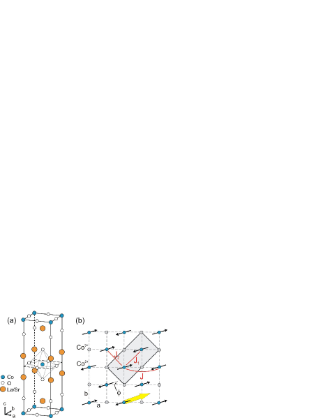
Figure 1: (Color online) (a) Tetragonal unit cell of La_2-xSr_xCoO₄. (b) Model for the charge and magnetic order within the $ab$ plane of La_3/2Sr_1/2CoO₄. The shaded rectangle is the magnetic unit cell. $\phi$ is the angle of the moments to the $a$ axis, with positive $\phi$ an anticlockwise rotation. The large (yellow) arrow represents the projection of the stacking vector ${\bf t}=(1.5,0.5,0.5)$ for the spin–charge order.

A preliminary report of a subset of the data presented here was given in Ref. Helme-PhysicaC-2004, , and as far as we are aware no other measurements of the magnetic excitations in La_3/2Sr_1/2CoO₄ have been published. Recently, however, there appeared a brief account of the magnetic excitation spectrum of La_3/2Ca_1/2CoO₄.Horigane-JMMM-2007 The data indicate that the energy scale of the magnetic excitations in the Sr-doped and Ca-doped cobaltates is very similar, but an important difference is that in La_3/2Ca_1/2CoO₄ there are ordered magnetic moments on both Co²⁺ the Co³⁺ sites.Horigane-JPSJ-2007 This increases the number of magnetic modes in the excitation spectrum and makes it harder to analyze. We also mention that the magnetic excitations have been studied in the isostructural half-doped compounds La_3/2Sr_1/2NiO₄ (Ref. Freeman-PRB-2005, ) and La_1/2Sr_3/2MnO₄ (Ref. Senff-PRL-2006, ).

The paper is organized as follows. After giving details of the experimental methodology and sample characterization we describe the results of polarized neutron diffraction measurements designed to refine the magnetic structure of La_3/2Sr_1/2CoO₄. We then present our inelastic neutron scattering measurements which represent the main body of the work. This is followed by an analysis of the magnetic spectrum in terms of a generalized spin-wave model. The paper ends with a discussion of the results and a summary of the main conclusions from the work.

II Experimental Details

Single crystals of La_3/2Sr_1/2CoO₄ were grown in Oxford by the optical floating-zone method in a four-mirror image furnace. The growth took place in a mixed Ar/O₂ atmosphere at a pressure of 7–9 bar. The feed and seed rods were scanned at a rate of 3–4 mm hr^-1 and counter-rotated at 30 r.p.m. Details of the preparation and crystal growth procedure are very similar to those used for La_1-xSr_xCoO_3+δ described in Ref. Prabhak-JCG-2005, . Two large crystals were prepared for the experiments. These were in the form of rods, approximately 10 mm in diameter and up to 80 mm in length. Several smaller crystals prepared under the same conditions were ground up into a fine powder and used for structural analysis by neutron powder diffraction. The general materials (GEM) diffractometer at the ISIS Facility was used to obtain the powder diffraction data. Basic information on the magnetic response of the crystals was obtained from magnetization measurements, which were performed on a superconducting quantum interference device (SQUID) magnetometer (Quantum Design).

Unpolarized neutron scattering measurements were made on the MAPS spectrometer at the ISIS Facility. MAPS is a time-of-flight chopper spectrometer with a large bank of pixelated detectors. The energy of the incident neutrons is selected by a Fermi chopper, which transmits pulses of neutrons with an energy bandwidth of typically 3–5 %. All the data presented here were obtained with an incident energy $E_{\rm i}$ of 50 meV and a chopper frequency of 350 Hz, giving an elastic energy resolution of 2 meV. The crystal used on MAPS was a single rod with a total mass of 35.5 g. Of this mass an estimated 24 g was in the neutron beam (which was smaller than the size of the crystal). The crystal was mounted with the rod axis approximately vertical, and aligned such that the tetragonal $c$ axis was parallel to the incident beam direction. Spectra were recorded at temperatures of 10 K, 60 K and 300 K. Measurements of a standard vanadium sample were used to normalize the spectra and place them on an absolute intensity scale.

Polarized neutron scattering measurements were made on the IN20 and IN22 triple-axis spectrometers at the Institut Laue-Langevin. On IN20, two crystals of masses 6.5 g and 5.5 g cut from the same rod were co-aligned with their rod axes parallel. Two settings of the sample were used, giving access to the $(hk0)$ and $(hhl)$ planes in reciprocal space [we refer crystallographic notation to the tetragonal unit cell shown in Fig. 1(a)]. For the IN22 experiment we used the 6.5 g crystal on its own and measured in just the second orientation. On both IN20 and IN22 we used the (111) Bragg reflection of Heusler alloy as both monochromator and analyzer and worked with a fixed final energy $E_{\rm f}$ of 14.7 meV. A graphite filter was placed after the sample to suppress higher harmonics in the scattered beam. Measurements employed uniaxial polarization analysis,Moon-PR-1969 and were made with three configurations of the neutron spin polarization $\bf P$ relative to the scattering vector $\bf Q$: (a) ${\bf P}\parallel{\bf Q}$, (b) ${\bf P}\perp{\bf Q}$ with $\bf P$ in the scattering plane, and (c) ${\bf P}\perp{\bf Q}$ with $\bf P$ perpendicular to the scattering plane. Data were collected in both the spin-flip (SF) and non-spin-flip (NSF) channels. Details of how the six measurements $\{({\rm a}),({\rm b}),({\rm c})\}\times\{{\rm SF},{\rm NSF}\}$ can be used to separate the components of a magnetic structure are given in Ref. Freeman-PRB-2002, .

III Results

III.1 Structural characterization

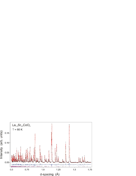
Figure 2: (Color online) Part of the Rietveld refinement for tetragonal La_1.5Sr_0.5CoO_4+δ at 60 K. Circles are data measured in the backscattering detector bank ($\langle 2\theta\rangle=154.5^{\circ}$) on GEM at ISIS. The solid (red) line shows the calculated profile fit. Tick marks show the positions of allowed reflections, and the solid (blue) line below the data shows the difference between the data and fit. The background fitted in the refinement was subtracted prior to plotting. The fit parameters are given in Table 1.

Neutron powder diffraction data collected on GEM at several temperatures were analyzed by Rietveld refinement using the GSAS suite of programs.GSAS Data from the three detector banks at highest scattering-angle were refined simultaneously. Refinements were made in the space group $I4/mmm$ for the parent structure whose unit cell is shown in Fig. 1(a). Attempts to refine the structure in the $Fmmm$ space group to allow the possibility of an orthorhombic distortion did not lead to any statistically-significant improvements in the quality of the fits. In addition to the atomic positions shown in Fig. 1(a), we also allowed for the possibility of interstitial oxygen at site $(0.5,0,0.25)$, where excess oxygen has previously been foundLeToquin-PhysicaB-2004 in La₂CoO_4+δ. In order to achieve convergence it was necessary to fix the thermal parameter ($U_{\rm iso}$) of this third oxygen site to be the same as that of the second oxygen site.

As an example, Fig. 2 shows the neutron powder diffraction pattern and refined profile fit for the data recorded in the highest-angle detector bank with the sample at a temperature of 60 K. The parameters for the refinement are listed in Table 1 together with those for the other temperatures at which measurements were made. The data at 2 K will have contained magnetic Bragg peaks which were not allowed for in the refinement. This probably explains the slightly higher value of $R_{\rm wp}$ for this temperature. Values for the lattice constants and atomic positions are in good agreement with previous data.Zaliznyak-PRB-2001 To within experimental accuracy the refinements show no deviation from stoichiometry in the oxygen content (i.e. $\delta=0$), and no evidence for any deviation from the nominal La:Sr ratio of 3:1.

Table 1: Structural parameters for La_1.5Sr_0.5CoO_4+δ at temperatures between 2 K and 300 K refined from neutron powder diffraction data. The refinements were performed in the tetragonal space group $I4/mmm$ of the parent structure with atomic positions La/Sr 4$e$ $(0,0,z_{\rm La})$, Co 2$a$ $(0,0,0)$, O(1) 4$c$ $(0.5,0,0)$, O(2) 4$e$ $(0,0,z_{\rm O2})$, O(3) 4$d$ $(0.5,0,0.25)$ in lattice units. The O(3) position is an interstitial site. $n$ is the occupancy of each site per formula unit and $U_{\rm iso}$ is the isotropic temperature factor. The occupancy of the Co site was not refined ($n=1$), and La/Sr site was constrained such that $n_{\rm La}+n_{\rm Sr}=2$. The numbers in parentheses are statistical errors in the last digit of the refined parameters. $R_{\rm wp}$ is the weighted profile residual function.

Temperature (K)		2	60	100	150	200	300
$a=b$	(Å)	3.83495(2)	3.83537(2)	3.83665(2)	3.83693(2)	3.83959(2)	3.84080(2)
$c$	(Å)	12.5235(1)	12.5239(1)	12.5277(1)	12.5287(1)	12.5413(1)	12.5481(1)
$V=abc$	(Å3)	184.181(2)	184.227(2)	184.406(2)	184.448(2)	184.890(2)	185.107(2)
La/Sr	$z_{\rm La}$	0.36216(2)	0.36214(2)	0.36216(2)	0.36215(2)	0.36217(3)	0.36216(3)
	$n_{\rm La}$	1.55(7)	1.59(7)	1.52(7)	1.51(7)	1.49(7)	1.47(7)
	$n_{\rm Sr}$	0.45(7)	0.41(7)	0.48(7)	0.49(7)	0.51(7)	0.53(7)
	$U_{\rm iso}\times 100$ (Å2)	0.219(7)	0.244(7)	0.300(7)	0.307(7)	0.419(8)	0.480(8)
Co	$U_{\rm iso}\times 100$ (Å2)	0.24(3)	0.24(3)	0.30(3)	0.29(3)	0.42(3)	0.43(4)
O(1)	$n$	2.01(1)	2.01(1)	2.00(1)	2.00(1)	2.00(1)	1.99(1)
	$U_{\rm iso}\times 100$ (Å2)	0.50(1)	0.52(1)	0.56(1)	0.57(1)	0.70(1)	0.75(1)
O(2)	$z_{O2}$	0.16967(4)	0.16968(4)	0.16968(3)	0.16967(4)	0.16977(4)	0.16981(4)
	$n$	1.98(1)	1.99(1)	1.98(1)	1.98(1)	1.98(1)	1.97(1)
	$U_{\rm iso}\times 100$ (Å2)	1.02(1)	1.06(1)	1.11(1)	1.12(1)	1.29(1)	1.37(2)
O(3)	$n$	0.012(2)	0.008(2)	0.008(2)	0.006(2)	0.004(2)	0.004(2)
	$U_{\rm iso}\times 100$ (Å2)	1.02(1)	1.06(1)	1.11(1)	1.12(1)	1.29(1)	1.37(2)
$\delta$		0.00(2)	0.00(2)	-0.01(2)	-0.02(2)	-0.02(2)	-0.03(2)
$R_{\rm wp}$	(%)	3.11	3.04	2.85	2.96	2.88	2.85

III.2 Magnetic structure

We first review the main characteristics of the magnetic and charge order in La_1.5Sr_0.5CoO₄ with the aid of the polarized-neutron diffraction measurements presented in Fig. 3. All the scans shown in this figure contain raw data recorded at 2 K on IN20 with the neutron polarization parallel to the scattering vector (${\bf P}\parallel{\bf Q}$). In this configuration the spin-flip scattering is entirely magnetic and the non-spin-flip scattering is entirely non-magnetic (i.e. structural). Since the neutron polarization is not perfect (the flipping ratio was $\sim 20$) there is a small amount of leakage from one channel to the other.

Figure 3(a) is a diagram of part of the $(h,k,0)$ plane in reciprocal space showing the in-plane wavevectors corresponding to the magnetic and charge order. Representative scans along various in-plane and out-of-plane directions are shown in Figs. 3(b)–(e). These data confirm that the charge order scattering is peaked at wavevectors ${\bf Q}_{\rm co}=(h+0.5,k+0.5,l)$, with $h$, $k$ and $l$ integers, and that the magnetic order is characterized by four slightly-incommensurate wavevectors ${\bf Q}_{\rm m}=(h+0.5,k+0.5,l)\pm(0.25-\epsilon,0.25-\epsilon,0)$ and $(h+0.5,k+0.5,l)\pm(-0.25+\epsilon,0.25-\epsilon,0)$, where $h$ and $k$ are integers and $l$ is an odd integer for the first pair of ${\bf Q}_{\rm m}$ and an even integer for the second pair. In our crystal $\epsilon=0.005\pm 0.001$. The peaks are considerably sharper in scans parallel to the $ab$ plane [e.g. Figs. 3(c) and (d)] than in scans made in the out-of-plane direction [Figs. 3(b) and (e)], but in all directions the peak widths are broader than the resolution. The correlation lengths for the charge and magnetic orders estimated from $\xi=1/\Gamma$, where $\Gamma$ is the half-width at half-maximum, are $\xi_{\rm co}^{ab}=23\pm 2$ Å, $\xi_{\rm co}^{c}=8\pm 1$ Å, $\xi_{\rm m}^{ab}=52\pm 2$ Å and $\xi_{\rm m}^{c}=12\pm 1$ Å. These values are consistent with those reported by Zaliznyak et al.Zaliznyak-PRL-2000 apart from $\xi_{\rm m}^{ab}$, which we find to be $\sim 30$% smaller. This could be because we did not attempt to correct the peak width for experimental resolution.

The two in-plane scans shown in Fig. 3(c) are at $l=0$, which is a minimum of the intensity modulation along $(0,0,l)$ — see Fig. 3(e). The widths of the peaks in Fig. 3(c) are roughly twice those in Fig. 3(d) which are at a maximum of the $(0,0,l)$ intensity modulation. This suggests that in addition to the dominant magnetic order there also exists a small volume fraction of magnetically ordered regions with an average size of $\sim 25$ Å in the $ab$ plane which are not correlated to the magnetic order on the adjacent layers.

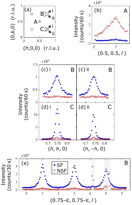
Figure 3: (Color online) Polarized neutron diffraction from magnetic and charge orders in La_1.5Sr_0.5CoO₄. (a) Diagram of the $(h,k,0)$ reciprocal lattice plane showing the in-plane wavevectors of the magnetic order (two twins, unfilled and filled circles marked B and C, respectively) and charge order (crossed circle marked A). The arrows indicate scan directions. (b) $l$-dependence of the charge-order peak at $(0.5,0.5,7)$. (c) and (d) In-plane scans through the magnetic ordering wavevectors in the directions indicated. (e) $l$-dependence of the intensity at the magnetic wavevector marked B. Shaded grey regions contain points contaminated with scattering from aluminium. All scans shown in this figure were made on IN20 with ${\bf P}\parallel{\bf Q}$ and recorded in both the spin-flip (SF, filled blue circles) and non-spin-flip (NSF, open red squares) channels. No corrections have been applied for the imperfect neutron polarization. The sample temperature was 2 K.

It is reasonable to assume that the short correlation lengths in the $c$ direction are caused by the existence of different stacking sequences with similar energy. Since both the charge and magnetic diffraction peaks are found at integer $l$ the majority stacking is periodic in the lattice. However, there are several ways in which the structure on adjacent layers can be related. To distinguish these experimentally let us consider the case where the magnetic structure is collinear, so that the spin–charge order on one layer (say $z=0$) can be related to that on the adjacent layer ($z=\frac{1}{2}$) by a translation ${\bf t}$. The structure factor for the spin and charge diffraction peaks then contains a factor $1+\exp(i{\bf Q}\cdot{\bf t})=1+\exp\{2\pi i(ht_{x}+kt_{y}+lt_{z})\}$, where $t_{x},t_{y},t_{z}$ are the components of $\bf t$ written as fractional coordinates along the crystallographic $a$, $b$ and $c$ axes.

We consider first the case ${\bf t}=(-0.5,0.5,0.5)$. For the structure shown in Fig. 1(b) this stacking leads to systematic absences at magnetic ordering wavevectors of the type $(0.25,0.25,l)$, $(0.75,0.75,l)$, etc, when $l$ is odd and for magnetic wavevectors of the type $(0.25,0.75,l)$, $(0.75,0.25,l)$, etc [associated with the twin obtained by rotating the structure in Fig. 1(b) by 90 deg — see Fig. 3(a)], when $l$ is even. These predictions are inconsistent with experiment — see Fig. 3(e). We next consider ${\bf t}=(0.5,0.5,0.5)$. In this case there are no magnetic absences, again inconsistent with experiment. We finally consider ${\bf t}=(1.5,0.5,0.5)$. For this case the systematic absences are at $(0.25,0.25,l)$, etc, when $l$ is even, and at $(0.25,0.75,l)$, etc, when $l$ is odd. This is consistent with the observations. The twinning ensures that there are no absences in the charge-order peaks, again consistent with experiment.Zaliznyak-PRL-2000 We conclude, therefore, that the most likely stacking vector is ${\bf t}=(1.5,0.5,0.5)$ (or its equivalent). This vector is shown in Fig. 1(b). With this stacking, spins in the $z=\frac{1}{2}$ layer are antiparallel to the closest spins in the $z=0$ and $z=1$ layers.

The fact that the magnetic and charge correlation lengths along the $c$ axis are so short suggests that the majority stacking is only slightly more favorable energetically than other possible stacking sequences. Therefore, the propagation of the structure along the $c$ axis is presumably interrupted frequently by stacking faults in which adjacent layers are related by different ${\bf t}$ vectors.

Let us now turn to the temperature evolution of the magnetic order. In Fig. 4 we show the magnetization of La_1.5Sr_0.5CoO₄ as a function of temperature, recorded with a relatively low measuring field $H$ of 100 Oe. The data are in very good quantitative agreement with the measurements reported in Refs. Moritomo-PRB-1997, and Hollmann-NJP-2008, , both of which employed a significantly higher measuring field. The magnetization exhibits strong $XY$-like anisotropy, as shown in the inset of Fig. 4, and there is a broad maximum in the in-plane response centered at about 60 K. At lower temperatures there is a splitting between the field-cooled (FC) and zero-field-cooled (ZFC) data. The splitting is largest for $H\parallel ab$.

Our measurements, however, reveal an additional feature. At approximately 31 K there is a sharp kink in the data. This kink marks the temperature below which the FC–ZFC splitting begins to open up most rapidly. The observation of this kink prompted us to perform polarized-neutron diffraction measurements to investigate whether there might be a change in the magnetic structure at 31 K.

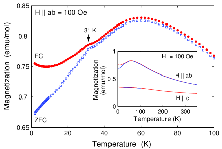
Figure 4: (Color online) Temperature dependence of the magnetization of La_1.5Sr_0.5CoO₄. The main frame shows measurements made with the applied field $H$ of strength 100 Oe ($\mu_{0}H=0.01$ T) applied parallel to the $ab$ plane. Red filled circles and blue open squares show data from field-cooled (FC) and zero-field-cooled (ZFC) measurements, respectively. Inset: data up to $T=350$ K showing measurements with both $H\parallel ab$ and $H\parallel c$.

We followed the approach described in Ref. Freeman-PRB-2002, (see also Ref. Helme-DPhil-2006, ). SF and NSF intensities were recorded at two magnetic Bragg peaks using three orthogonal directions of the neutron polarization $\bf P$. Measurements were made on both IN20 and IN22, and corrections were applied to the measured intensities to compensate for the imperfect polarization. The two Bragg peaks used were ${\bf Q}_{1}=(0.25+\epsilon,0.25+\epsilon,7)$ and ${\bf Q}_{2}=(1.25+\epsilon,1.25+\epsilon,1)$. These were chosen because they make small angles (less than 10 deg) to the $c$ axis and $[110]$ direction, respectively, which reduces the uncertainty in the values of the spin components derived by this method. For example, if ${\bf Q}_{1}$ could be chosen exactly parallel to $c$ then the Bragg peak intensities measured at ${\bf Q}_{1}$ would be independent of the magnetic component along the $c$ axis.

Because ${\bf Q}_{1}$ and ${\bf Q}_{2}$ lie in the $(h,h,l)$ plane the magnetic scattering at these wavevectors is naturally described in terms of the intensities scattered by the projection of the ordered moments along the orthogonal directions $[1,1,0]$, $[1,-1,0]$ and $[0,0,1]$. We call these intensities $I_{110}$, $I_{1\bar{1}0}$ and $I_{c}$, respectively. The expressions in Table I of Ref. Freeman-PRB-2002, can be used to determine the ratios $I_{110}/I_{1\bar{1}0}$ and $I_{c}/(I_{110}+I_{1\bar{1}0})$ from the sets of measurements at ${\bf Q}_{1}$ and ${\bf Q}_{2}$. The latter ratio was found to be less than 0.01 at all temperatures. The assumption that the intensities are proportional to the squares of the ordered moments constrains the angle of the moments to the $ab$ plane to $<5$ deg. Given the strong planar anisotropy it is safe to assume that the moments lie in the $ab$ plane.

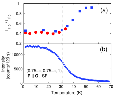
Figure 5: (Color online) Development of magnetic order in La_1.5Sr_0.5CoO₄. (a) Ratio of the intensities scattered by the projection of the ordered moments along the $[110]$ and $[1\bar{1}0]$ directions. Data are from IN20 (filled red circles) and IN22 (filled blue squares). (b) Intensity of the $(0.75-\epsilon,0.75-\epsilon,1)$ magnetic Bragg peak. The broken grey line marks the position of the kink in the magnetization (see Fig. 4).

In Fig. 5(a) we plot the ratio $I_{110}/I_{1\bar{1}0}$ as a function of temperature. At temperatures below 30 K, $I_{110}/I_{1\bar{1}0}$ is approximately constant with a value of 0.4. On warming above 30 K this ratio gradually increases until at $\sim 50$ K it approaches 1. This indicates one of two things. Either (i) there are two (or more) spin domains which contribute to each magnetic Bragg peak, and on cooling one of these domains becomes preferentially populated, or (ii) there is a spin-canting transition reminiscent of that proposed to occur in the isostructural layered nickelates.Freeman-PRB-2002 ; Lee-PRB-2001 ; Freeman-PRB-2004 ; Giblin-PRB-2008 We consider these possibilities further in Section V

Figure 5(b) shows the temperature dependence of the intensity of the $(0.75-\epsilon,0.75-\epsilon,1)$ magnetic peak. The slow increase in intensity on cooling starts in the vicinity of the broad hump in the magnetization at $\sim 60$ K, confirming that the hump is associated with the build-up of magnetic correlations. We have indicated on Figs. 5(a) and (b) the temperature at which the kink is observed in the magnetization. There is no obvious anomaly in the magnetic peak intensity at this temperature, but the data in Fig. 5(a) indicate that the 31 K kink marks the temperature below which the magnetic structure stops changing.

III.3 Magnetic excitations

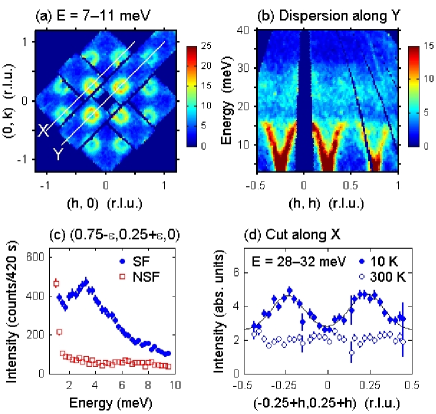
Figure 6: (Color online) Spin excitation spectrum of La_1.5Sr_0.5CoO₄. (a) Map of the intensity within the $(h,k)$ plane averaged over the energy range $7-11$ meV, measured with a sample temperature of $T=10$ K . The circles centered on the magnetic ordering wavevectors are due to scattering from dispersive magnetic excitations. (b) Energy–$\bf Q$ slice showing the dispersion along the line Y in (a). (c) Energy scan at the magnetic ordering wavevector $(0.75-\epsilon,0.25+\epsilon,0)$ with neutron polarization analysis to separate the magnetic scattering in the spin-flip (SF) channel from the non-magnetic scattering in the non-spin-flip (NSF) channel. The data were obtained on IN20 at $T=2$ K and reveal an energy gap of $\sim 3$ meV in the magnetic spectrum. (d) Scans along the line X in (a) at temperatures of 10 K and 300 K averaged over the energy range $28-32$ meV confirming the existence of magnetic modes at this energy. The data in (a), (b) and (d) were recorded on MAPS, and the intensity is in units of mb sr^-1 meV^-1 f.u.^-1, where “f.u.” stands for “formula unit” (of La_1.5Sr_0.5CoO₄).

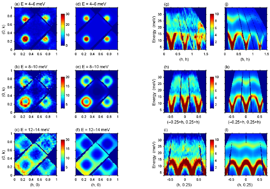
Figure 7: (Color online) Intensity maps of measured and simulated neutron scattering from La_1.5Sr_0.5CoO₄. The data are from MAPS, and the simulations are obtained from the many-level spin-wave model discussed in the text with Co${}^{2+}-$Co²⁺ exchange interactions $J=1.4$ meV and $J_{1}=J_{2}=0$ [see Fig. 1(b)]. (a)–(f) Constant-energy slices averaged over the energy ranges indicated. (g)–(l) Energy–$\bf Q$ slices showing the dispersion along the three symmetry directions indicated. The intensity scale is in units of mb sr^-1 meV^-1 f.u.^-1.

Figure 6 provides an overview of the magnetic spectrum. The intensity map presented in Fig. 6(a) is a slice from a MAPS data volume, averaged over the energy range $7-11$ meV and projected onto the $(h,k)$ plane. The image shows dispersive magnetic excitations emerging from the magnetic ordering wavevectors. The rings of scattering correspond to the intersection of the constant-energy slice plane with the spin-wave cones. Figure 6(b) is an energy-wavevector slice through the same data volume showing the dispersion along a line parallel to $(h,h,0)$. The spectrum is dominated by an intense band of scattering extending up to 16 meV. There is also a weaker band of scattering in the range $20-30$ meV which is more diffuse than that of the lower band but which disperses with the same period.

Figure 6(c) is an energy scan performed on IN20 with the wavevector fixed at the magnetic ordering wavevector ${\bf Q}_{m}=(0.75-\epsilon,0.25+\epsilon,0)$. The two sets of points are the neutron spin-flip (SF) and non-spin-flip (NSF) signals. In the ${\bf P}\parallel{\bf Q}$ configuration used for this measurement the SF channel contains only magnetic scattering, so the large signal in the SF data is scattering from magnetic excitations and reveals a gap of approximately 3 meV in the low-energy spin-wave band. Having observed the gap we performed constant-energy scans (not shown) along $(0.75-\epsilon,0.75-\epsilon,l)$ from $l=0$ to 2 at energies of 2 meV and 4 meV, i.e. just below and just above the gap. At 2 meV there remained a modulation in the magnetic scattering along the scan with a broad maximum at the magnetic Bragg peak position $(0.75-\epsilon,0.75-\epsilon,1)$, whereas at 4 meV the scan was featureless to within the experimental precision of $\sim 5$%. This implies that for energies above 4 meV the magnetic dynamics are completely uncorrelated along the $c$ axis and the spectrum can be considered as two-dimensional.

To help understand the origin of the gap we performed neutron polarization analysis at energies of 2 meV and 4 meV. For each energy we recorded the signal in the same three polarization channels and at the same two wavevectors ${\bf Q}_{1}=(0.25+\epsilon,0.25+\epsilon,7)$ and ${\bf Q}_{2}=(1.25+\epsilon,1.25+\epsilon,1)$ as used to analyze the magnetic order (see Section III.2). The signal in each polarization channel can be written in terms of the response functions $S^{110}({\bf Q}_{j},\omega)$, $S^{1\bar{1}0}({\bf Q}_{j},\omega)$ and $S^{zz}({\bf Q}_{j},\omega)$ for magnetic fluctuation components parallel to $[110]$, $[1\bar{1}0]$, and parallel to the $c$ axis ($z$ direction), respectively. Here, $\omega$ is the neutron energy transfer and $j=1,2$ indexes the two magnetic wavevectors. Applying the same analysis as used to separate diffraction from different components of the ordered momentsFreeman-PRB-2002 ; Helme-DPhil-2006 we find at $T=2$ K,

$$S^{zz}({\bf Q}_{j},2{\rm\,meV})/S^{1\bar{1}0}({\bf Q}_{j},2{\rm\,meV}) = -0.04\pm 0.06$$

$$S^{zz}({\bf Q}_{j},4{\rm\,meV})/S^{1\bar{1}0}({\bf Q}_{j},4{\rm\,meV}) = -0.02\pm 0.04$$

$$S^{110}({\bf Q}_{j},2{\rm\,meV})/S^{1\bar{1}0}({\bf Q}_{j},2{\rm\,meV}) = 1.19\pm 0.07$$

$$S^{110}({\bf Q}_{j},4{\rm\,meV})/S^{1\bar{1}0}({\bf Q}_{j},4{\rm\,meV}) = 1.00\pm 0.05\ .$$

The first two ratios show that the spin fluctuations at both 2 meV and 4 meV are restricted to the $ab$ plane. This is consistent with the strong $XY$-like anisotropy of this system and implies that the gap is due to a small single-ion or exchange anisotropy within the $ab$ plane. The third and fourth ratios show that the strengths of the fluctuations in the $[110]$ and $[1\bar{1}0]$ directions are roughly equal in this energy range.

In Fig. 6(d) we show cuts through the MAPS data averaged over the energy range 28 meV to 32 meV, which is near the top of the weak upper band of excitations. The scan at 10 K shows a sinusoidal intensity modulation along the cut direction [line X in Fig. 6(a)], whereas the scan at 300 K is flat and always below the 10 K data. The observation that the signal goes away on raising the temperature from 10 K to 300 K shows conclusively that it is magnetic in origin, because the scattering from phonons would increase in intensity.

To give a more comprehensive picture of the magnetic excitation spectrum we present in Fig. 7 a further series of slices through the MAPS data. The data have been averaged over symmetry-equivalent directions to improve the statistics, and are plotted with respect to the two-dimensional reciprocal lattice of the CoO₂ layers indexed by $(h,k)$. In the time-of-flight method the out-of-plane wavevector component $l$ varies with energy and also varies across the detector for a fixed energy. However, because the magnetic dynamics is two-dimensional (for energies greater than $\sim$4 meV) the magnetic dispersion does not depend on $l$ and the intensity of the spectrum varies only slowly with $l$. The $l$ dependence of the intensities of the modes is correctly taken into account in the models presented in Section IV.

Figures 7(a)–(c) are constant-energy slices averaged over a 2 meV interval centered on 5 meV, 9 meV and 13 meV. These illustrate how the lower spin-wave band disperses away from the magnetic zone centers. Figures 7(g)–(i) display three energy–wavevector slices taken along different symmetry directions in the Brillouin zone. The intense lower band and weak upper band are clearly seen in each of these slices.

To facilitate comparison with models we took cuts through the MAPS data set along several symmetry directions and extracted points describing the dispersion. The magnetic dispersion obtained from the MAPS data is displayed in the upper panel of Fig. 8. The points are obtained either from wavevector cuts at fixed energy, or from energy cuts at fixed wavevector. Peaks in the cuts were fitted with Lorentzian functions on a linear background. The points representing the energy gap at the magnetic zone centres were estimated from the data in Fig. 6(c).

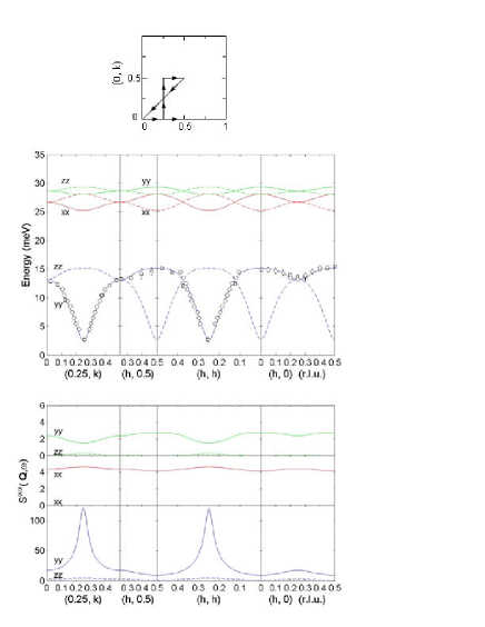
Figure 8: (Color online) Dispersion of magnetic excitations in La_1.5Sr_0.5CoO₄. The diagram at the top shows the path in reciprocal space along which the dispersion is plotted. The middle figure shows the measured and calculated dispersion. Symbols are from fits to the experimental data. Circles are from constant-energy cuts, squares and diamonds are from constant-wavevector cuts. The lines are calculated from the many-level spin–orbital model with Co${}^{2+}-$Co²⁺ exchange interactions $J=1.4$ meV and $J_{1}=J_{2}=0$ [see Fig. 1(b)]. The lower figure displays the calculated response functions $S^{\alpha\alpha}({\bf Q},\omega)$ for each mode shown in the dispersion plot. The labels on the curves give the $\alpha\alpha$ components for the case where the ordered moments point along $x$.

IV Analysis

Figure 9: Single-ion energy levels of the ${}^{4}F$ term of Co²⁺ in La_1.5Sr_0.5CoO₄, showing how the term splits when successively smaller interactions are added. The splitting caused by the axially-distorted crystal field is obtained with coefficients $B_{2}^{0}=13$ meV, $B_{4}^{0}=-1.4$ meV and $B_{4}^{4}=-8$ meV for the Stevens operator equivalents $O_{2}^{0},O_{4}^{0}$ and $O_{4}^{4}$. These values are approximately twice those calculated from the point-charge model. The right-most scheme includes spin–orbit coupling and shows the splitting of the lowest orbital quasi-triplet on an expanded vertical scale. The spin–orbit coupling parameter is $\lambda=-18.7$ meV.

The essential physics governing the magnetic properties of La_1.5Sr_0.5CoO₄ can be understood with reference to Fig. 9, which is an energy-level diagram for the high-spin state of Co²⁺ (3$d^{7}$, $L=3$, $S=3/2$) in an axially-distorted octahedral crystal field. A perfect octahedral field splits the orbital levels into two triplets and a singlet, and the small axial elongation of the octahedron splits each triplet into a singlet and a higher-lying doublet. Inclusion of spin–orbit coupling lifts the fourfold spin degeneracy of each of the orbital levels, splitting the ground state into two doublets. For realistic crystal field and spin–orbit interactions the two doublets are separated by approximately 25 meV, as we show later. Because the orbital ground state in the main octahedral field is a quasi-triplet it contains significant unquenched orbital angular momentum which is responsible for the strong planar anisotropy. As we shall see, the magnetic spectrum in the energy range probed in this study involves the lowest two doublets and is strongly influenced by the in-plane anisotropy and the unquenched orbital angular momentum.

The neutron scattering cross section for spin-only scattering, or for spin and orbital scattering in the dipole approximation, may be written Squires

$$\frac{{\rm d}^{2}\sigma}{{\rm d}\Omega{\rm d}E_{\rm f}} = \frac{k_{\rm f}}{k_{\rm i}}\left(\frac{\gamma r_{0}}{2}\right)^{2}f^{2}(Q)\exp(-2W)$$ (1)

$$\hskip 5.0pt\times\sum_{\alpha\beta}(\delta_{\alpha\beta}-\hat{Q}_{\alpha}\hat{Q}_{\beta})S^{\alpha\beta}({\bf Q},\omega),$$

where $(\gamma r_{0}/2)^{2}=72.8$ mb, $f(Q)$ is the magnetic form factor of Co²⁺, $\exp(-2W)$ is the Debye–Waller factor which is close to unity at low temperatures, $\hat{Q}_{\alpha}$ is the $\alpha$ component of a unit vector in the direction of $\bf Q$, and $S^{\alpha\beta}({\bf Q},\omega)$ is the response function describing $\alpha\beta$ magnetic correlations. In calculating the cross-section we average over an assumed 50:50 ratio of the two magnetic domains related to one another by a 90 deg rotation.

Putting the orbital angular momentum to one side for a moment, we can as a first approximation follow the standard route and attempt to describe the low-energy magnetic dynamics in the antiferromagnetic phase in terms of linear spin-wave excitations of an effective spin–$\frac{1}{2}$ model for the ground state doublet. We assume the collinear magnetic structure shown in Fig. 1 with spins along the $a$ axis ($\phi=0$). We consider a spin-only Hamiltonian and incorporate the magnetic anisotropy via anisotropic exchange interactions between effective $S=\frac{1}{2}$ spins. The Hamiltonian may be written

$${\mathcal{H}}=\sum_{\langle jk\rangle}\sum_{\alpha}J_{jk}^{\alpha}\,S_{j}^{\alpha}S_{k}^{\alpha}.$$ (2)

The first summation is over Co${}^{2+}-$Co²⁺ pairs with each pair counted only once, and the second summation is over the spin components $\alpha=x,y,z$. The $J_{jk}^{\alpha}$ are the exchange parameters. We include only $J$, $J_{1}$ and $J_{2}$ as defined in Fig. 1. $J$ acts in a straight line through the Co³⁺ site, whereas $J_{1}$ and J₂ have 90 deg paths. As we shall see, $J_{1}$ and $J_{2}$ are very much smaller than $J$, and so as a simplification we take $J_{1}$ and $J_{2}$ to be isotropic. For later convenience we write the anisotropy in $J$ in the form $J^{x}=J(1+\varepsilon)$, $J^{y}=J$ and $J^{z}=J(1-\delta)$ so that $\varepsilon$ and $\delta$ parameterize the degree of in-plane and out-of-plane anisotropy, respectively.

The theoretical expressions for the spin-wave dispersion and response functions are given in the Appendix, Eqs. (4)–(LABEL:App-eq5). For each wavevector there are two modes which are degenerate in the absence of anisotropy. Inclusion of easy-plane anisotropy lifts the degeneracy so that one mode ($\omega_{1}$) is associated with in-plane fluctuations and the other mode ($\omega_{2}$) is associated with out-of-plane fluctuations. At the magnetic Bragg peak wavevectors $(0.25,0.25)$, $(0.75,0.75)$, etc. the out-of-plane mode is gapped while the in-plane mode is gapless. The addition of a small in-plane anisotropy gaps the in-plane mode too. In our case we require a large out-of-plane anisotropy to describe the data. To see this we refer to the scattering intensity maps, e.g. Fig. 7(g), and the dispersion data in Fig. 8. If the anisotropy were small then the dispersion would reach a maximum at, or very close to, the magnetic zone boundaries $(0.125,0.125)$, $(0.375,0.375)$, etc. However, the measured dispersion reaches a maximum not at these positions but at the zone centres $(0,0)$, $(0.5,0.5)$, etc. This behavior can be reproduced in the linear spin-wave model only if there is substantial easy-plane anisotropy, i.e. if $J^{z}$ is significantly less than $J^{x}$ and $J^{y}$.

We found that the observed dispersion for the lower energy modes can be described very well throughout the Brillouin zone by the effective spin–$\frac{1}{2}$ spin-wave model with parameters $SJ=3.3$ meV, $J_{1}=J_{2}=0$, $\delta=0.65$ and $\varepsilon=0.03$. The zero values of the 90 deg exchange parameters $J_{1}$ and $J_{2}$ means that the magnetic structure consists of two uncoupled, interpenetrating, square-lattice antiferromagnets with spacing $2a$ on the CoO₂ layers. This is surprising and has important implications for the stability of the magnetic structure, so let us examine the evidence for this finding carefully.

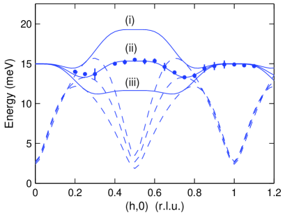
Figure 10: (Color online) Magnetic dispersion parallel to the $(h,0)$ direction in La_1.5Sr_0.5CoO₄. The symbols are points determined from energy cuts at constant wavevector through the MAPS data. Full and broken lines are in-plane and out-of-plane modes of the effective spin–$\frac{1}{2}$ ground-state doublet calculated from Eq. (2) by linear spin-wave theory with the following exchange parameters: (i) $SJ=3.68$ meV, $J_{1}=J_{2}=-J/2$; (ii) $SJ=3.23$ meV, $SJ_{1}=SJ_{2}=-0.15$ meV; (iii) $SJ=2.85$ meV, $J_{1}=J_{2}=J/2$. The parameters in (ii) have been adjusted to give the best fit to the data. In each case the exchange-anisotropy parameters were $\varepsilon=0.03$ and $\delta=0.65$.

First of all we show in Fig. 10 the measured dispersion along the $(h,0)$ line in reciprocal space. If the tetragonal symmetry is preserved in the charge-ordered phase then one expects $J_{1}=J_{2}$, which will tend to frustrate the magnetic order. If $J_{1}$ and $J_{2}$ are both antiferromagnetic then the effect on the dispersion relation is to soften the in-plane mode at the zone boundaries along the $(h,0)$ and $(0,k)$ directions. If $J_{1}$ and $J_{2}$ are both ferromagnetic then the softening is instead at the reciprocal lattice vectors. In both cases, therefore, we should observe a difference between the magnon energy at $(0.5,0)$ and at $(1,0)$. It can be seen from the data points in Fig. 10 that if such a difference exists then it is very small. To be more quantitative we plot on Fig 10 the dispersion curves calculated from linear spin-wave theory for the cases $J_{1}=J_{2}=J/2$ ($J$, $J_{1}$, $J_{2}$ all antiferromagnetic) and $J_{1}=J_{2}=-J/2$ ($J$ antiferromagnetic, $J_{1}$, $J_{2}$ ferromagnetic), adjusting the value of $J$ to accord with the data at $(1,0)$. These curves fall respectively well below and well above the experimental data, showing that the magnitudes of $J_{1}$ and $J_{2}$ must be considerably less than half that of $J$. The third curve plotted in Fig 10 is obtained with the parameters $SJ=3.23$ meV, $SJ_{1}=SJ_{2}=-0.15$ meV, and with $\delta=0.65$ and $\varepsilon=0.03$ as found earlier. This set of parameters gives the best fit to the data given the constraints, but is only a marginal improvement on the case $J_{1}=J_{2}=0$.

In the more general case where charge-order leads to orthorhombic symmetry, $J_{1}$ and $J_{2}$ could be different. Let us therefore consider the case where $J$ and $J_{1}$ are antiferromagnetic and $J_{2}$ is ferromagnetic, consistent with the structure in Fig. 1(b). This also creates differences between the magnon energies at $(0.5,0)$ and at $(1,0)$, and in addition it increases the energy of the in-plane mode at wavevectors such as $(0.25,0.75)$ and $(0.75,0.25)$. Neither of these effects is observed experimentally.

The spin-wave model just described succeeds in giving a good description of the dispersion of the lowest energy branches of the magnetic excitation spectrum and provides compelling evidence that the magnetism in La_1.5Sr_0.5CoO₄ is dominated by 180 deg Co${}^{2+}-$Co²⁺ exchange interactions. However, this model fails in two respects. First, it does not account for the band of magnetic scattering observed in the range $20-30$ meV, and second it cannot predict the correct intensities of the modes because it ignores orbital angular momentum.

The effective spin–$\frac{1}{2}$ model takes for its basis the eigenfunctions of $S_{x}$, where $x$ is the spin quantization direction. When single-ion anisotropy is strong and the true spin is greater than $\frac{1}{2}$, as we have here, there can be significant admixing of the basis states. This means that excitations to higher single-ion levels can propagate and can be observed by neutron scattering. Moreover, when the single-ion states contain a non-negligible orbital component this needs to be included for an accurate calculation of the neutron cross section, because the neutron couples to both the spin and the orbital angular momentum.

To achieve a more complete description of the magnetic spectrum we use a more realistic linear spin-wave formulation which takes as its basis the product states $|L_{x}S_{x}\rangle$ and determines the single-ion states self-consistently through the action of the crystal and exchange fields and the spin–orbit coupling. The method follows closely the approach described in Ref. Buyers-JPC-1971, in connection with the dispersive magnetic excitations of antiferromagnetic KCoF₃. Similar calculations have been done for CoO (Refs. Sakurai-PR-1968, and Tomiyasu-JPSJ-2006, ) and for CoF₂ (Ref. Allen-PRB-1971, ), the latter though without explicit inclusion of the orbital angular momentum.

The Hamiltonian for the coupled 3$d$ states of Co²⁺ (3$d^{7}$, $L=3$, $S=3/2$) in the distorted octahedral ligand field in La_1.5Sr_0.5CoO₄ is taken to be

$${\mathcal{H}} = \sum_{\langle jk\rangle}J_{jk}{\bf S}_{j}\cdot{\bf S}_{k}+\sum_{j}\left[\sum_{l,m}B_{l}^{m}O_{l}^{m}({\bf L}_{j})+\lambda{\bf L}_{j}\cdot{\bf S}_{j}\right].$$

The first term is an isotropic Heisenberg superexchange interaction between true spins $S=\frac{3}{2}$, and the second and third terms describe the single-ion crystal (ligand) field and spin–orbit interactions, respectively. The crystal field interaction is assumed to be the source of magnetic anisotropy, and any anisotropy in the exchange interactions is neglected. The $O_{l}^{m}$ are Stevens operator equivalents with $B_{l}^{m}$ the corresponding crystal-field parameters, and $\lambda$ is the spin–orbit coupling parameter. We used the value $\lambda=-18.7$ meV recently obtained from optical spectroscopy of CoO.Kant-PRB-2008 The axially-distorted octahedral crystal field is represented by the Stevens operators $O_{2}^{0}$, $O_{4}^{0}$ and $O_{4}^{4}$, where the quantization direction is taken along the tetragonal axis. We used the point charge modelHutchings-SSP-1964 to make a first estimate of the crystal-field parameters, using the data in Table 1 for the average Co–O bond lengths and the results of Ref. Zaliznyak-PRB-2001, for the oxygen displacements due to charge order, which slightly reduces the axial distortion of the octahedron. This predicted a total splitting of the 3$d^{7}$ ${}^{4}F$ term of about 800 meV (the small admixture of higher terms was neglected). The crystal-field splitting in La_1.5Sr_0.5CoO₄ has not been measured, but optical measurements of several compounds containing octahedrally-coordinated CoO₆ complexes show a typical splitting of about 2 eV.Abragam ; Pratt-PR-1959 This indicates that the point-charge parameters are about a factor 2 too small, so for an initial estimate we doubled the point-charge values, giving $B_{2}^{0}=9.3$ meV, $B_{4}^{0}=-1.35$ meV and $B_{4}^{4}=-8.0$ meV. We note that with this crystal field the ground state has $XY$-like anisotropy, as observed experimentally. The ground to first-excited doublet-doublet splitting is not very sensitive to the $B_{4}^{0}$ and $B_{4}^{4}$ parameters, but varies strongly with $B_{2}^{0}$. We therefore adjusted $B_{2}^{0}$ to obtain a good fit to the experimental data.

The method for diagonalizing (LABEL:Eq3) is described in the Appendix. To compare the many-level spin–orbital model with the data we fixed $J_{1}=J_{2}=0$, since we have already established that these parameters are very small, and allowed only the parameters $J$ and $B_{2}^{0}$ to vary. The best agreement was obtained with $B_{2}^{0}=13.0$ meV and $J=1.4$ meV. A small anisotropy-field term ${\bf H}_{a}\cdot{\bf S}$ with ${\bf H}_{a}$ directed along the $x$ axis and of magnitude 0.22 meV was added to (LABEL:Eq3) to fix the direction of the ordered moments and to reproduce the observed in-plane spin gap of $\sim$3 meV. The dispersion relations and response functions calculated with these parameters are shown in Fig. 8. The calculated dispersion for the low-energy branches is virtually indistinguishable from that calculated from the effective spin–$\frac{1}{2}$ model described earlier and agrees very well with the experimental data. We note that when $J_{1}=J_{2}=0$ the magnetic dispersion is the same for the two twins of the assumed magnetic structure [Fig. 1(b)] whose propagation vectors are related by a 90^∘ rotation. This means that the analysis of the excitation spectrum is not affected by the twinning.

The many-level spin–orbital model allows us to go beyond the lowest two magnon branches and examine the modes derived from the upper doublet in the single-ion spectrum (Fig. 9). The model predicts two pairs of dispersive bands between 25 meV and 30 meV as shown in the middle panel of Fig. 8. In the lower panel of Fig. 8 it can be seen that two out of these four modes have non-negligible response functions. Interestingly, the mode with strongest intensity is a longitudinal excitation, labeled $xx$ in Fig. 8, and is therefore very different in character to a conventional spin precession wave.

In Fig. 7 we show neutron scattering intensity maps calculated with the many-level spin–orbital model alongside the corresponding experimental data. The presented intensity is $(k_{i}/k_{f})\,{\rm d}^{2}\sigma/{\rm d}\Omega{\rm d}E_{\rm f}$, i.e. the scattering cross section in absolute units as defined in Eq. 1 multiplied by the factor $k_{i}/k_{f}$. The simulations properly take into account the variation in the scattering vector $\bf Q$ with position on the detector and with energy, and the intensity has been averaged over equivalent 90 deg magnetic domains. The simulated spectra were convoluted with a Lorentzian broadening function with a full-width at half maximum of 4 meV to take into account the spectrometer resolution ($\simeq 2$ meV) and intrinsic broadening, and have been multiplied by a constant scale factor of 0.3 to obtain quantitative agreement with the experimental data. We estimate that absorption and self-shielding in the sample accounts for a factor of about 0.5, and a further reduction of order 10% may be expected due to zero-point magnetic fluctuations not included in the model. Therefore, the known corrections account for a scale factor of about 0.45, which is somewhat larger than the applied scale factor of 0.3.

Overall, the simulations from the many-level spin–orbital model provides an excellent description of the observed magnetic excitation spectrum in the measured energy range. With a realistic crystal field and only two free parameters in the Hamiltonian ($J$ and $B_{2}^{0}$) plus an overall scale factor the simulations reproduce the dispersion and intensities of the all the observed modes in the spectrum extremely well.

V Discussion

The experiments presented here have shown that both the magnetic order and the magnetic excitation spectrum of charge-ordered La_1.5Sr_0.5CoO₄ can be understood in terms of a square, two-sublattice, collinear antiferromagnet, with ordered moments localized on the Co²⁺ ions and pointing in the CoO₂ layers. The two lowest-frequency branches of the magnetic excitation spectrum are conventional spin-precession waves, but higher-frequency dispersive modes are of different character. In particular, a branch observed at $\sim 25$ meV is found to correspond to propagating magnetic fluctuations which are longitudinal relative to the ordered moment direction.

To arrive at this point, proper account has had to be taken of the orbital component in the ground state, which is not negligible. For example, from the self-consistent solution of the mean-field equations (8) we calculate the spin and orbital components of the ordered moment to be 2.69 $\mu_{\rm B}$ and 1.12 $\mu_{\rm B}$, respectively. The unquenched orbital component has also been shown to be important for achieving a quantitative understanding of the bulk susceptibility.Hollmann-NJP-2008 The total ordered moment in the model of 3.8 $\mu_{\rm B}$ is rather larger than the experimentally-determined ordered moment of 2.9 $\mu_{\rm B}$ (Ref. Zaliznyak-PRL-2000, ). It is not clear why these values should differ, but if confirmed then this difference could be the reason why the calculated spectrum has a higher overall intensity than the measured spectrum.

Perhaps the most surprising result to emerge from the analysis of the spin excitation spectrum is the virtual absence of the 90 deg Co²⁺–Co³⁺–Co²⁺ exchange couplings $J_{1}$ and $J_{2}$ relative to the 180 deg coupling $J$. This is dramatically counter to the simplest estimate $J_{1}\sim J_{2}\sim 2J$ based on exchange paths involving a single Co³⁺ bonding orbital,Zaliznyak-PRL-2000 and implies that frustration effects on the magnetic order are very small. One consequence is that the magnetic structure can be regarded as two interpenetrating, square-lattice, antiferromagnets with spacing $2a$. In the complete absence of $J_{1}$ and $J_{2}$ the moment directions for the two interpenetrating antiferromagnets would be unrelated to one another, but quantum fluctuations are expected to stabilize collinear order of the global magnetic system via the order-by-disorder mechanism.Kim-PRL-1999 A study of the spin wave spectrum of stripe-ordered La_2-xSr_xNiO₄ similarly concluded that the 180 deg Ni²⁺–Ni²⁺ exchange was significantly larger than the 90 deg coupling.Wu-PRB-2005 Given the importance of exchange for the stability of spin- and charge-ordered ground states it would be of interest to seek an understanding the exchange interactions in these systems in terms of the bonding orbitals involved.

There remain some details of the magnetic order to be understood. In Fig. 5(a) we reported how the ratio $I_{110}/I_{1\bar{1}0}$ increases from approximately 0.4 to almost 1.0 in the temperature range $30-50$ K, and in Fig. 4 we see that the start of this increase coincides with a kink in the magnetization below which the field-cooled and zero-field-cooled magnetization separate. To these observations we add a recent finding from a muon-spin rotation ($\mu$SR) study Giblin-unpublished that the kink coincides with the temperature at which magnetic ordering sets in on the muon timescale ($\sim 10^{-6}$ s). Since $\mu$SR and bulk magnetization probe much longer timescales than neutron diffraction ($\sim 10^{-12}$ s) we can take 31 K to be the static magnetic ordering temperature. Between 31 K and $\sim 60$ K magnetic Bragg peaks are still observed by neutron diffraction and so in this temperature range the magnetic order is not static but fluctuates on a timescale between $\sim 10^{-6}$ and $\sim 10^{-12}$ s.

For the assumed collinear magnetic structure there are several possible ways to explain the behavior of $I_{110}/I_{1\bar{1}0}$. One is in terms of a canting of the moments. If the moments point along the $a$ or $b$ direction then $I_{110}/I_{1\bar{1}0}=1$, but if they make an angle greater than 45 deg to $[110]$ then $I_{110}/I_{1\bar{1}0}<1$ [note that we are referring here to the domain in which the modulation of the magnetic structure is along $[110]$ — see Fig. 1(b)]. The observed low temperature value of $I_{110}/I_{1\bar{1}0}=0.4$ corresponds to a turn-angle of 12 deg. According to this model, therefore, the moments point along the $a$ (or $b$) direction when they first start to order, but gradually turn towards the $[1\bar{1}0]$ direction (i.e. away from the modulation direction) on cooling. By $\sim 30$ K the moments have turned through an angle of about 12 deg, i.e. in Fig. 1(b) $\phi=-12$ deg or $+102$ deg, and they remain at this angle at lower temperatures. Although consistent with the data, this model requires an explanation for what causes the rotation of the ordered moments and for why they fix on a canting angle of 12 deg from the Co–O bond directions at low temperatures.

Another possible interpretation of the $I_{110}/I_{1\bar{1}0}$ data is in terms of a change in population of different inequivalent spin domains. For example, if the easy magnetic direction within the plane were at 45 deg to the Co–O bonds, i.e. $\phi=\pm 45$ deg in Fig. 1(b), then in the ordered phase the moments could in principle point either parallel or perpendicular to the in-plane modulation direction of the structure. These longitudinal and transverse structures are not related by symmetry so their energies will in general differ. If the energy of the transverse structure were the lower of the two then the transverse structure would be present in greater proportion at the temperature of $\sim 30$ K when static order sets in, resulting in $I_{110}/I_{1\bar{1}0}<1$. With increasing temperature above $\sim 30$ K thermal fluctuations would tend to equalize the populations of the two domains, consistent with the observed increase in $I_{110}/I_{1\bar{1}0}$. The difference between the field-cooled and zero-field-cooled magnetization below $30$ K may be caused by the effect of the magnetic field favoring one domain over the other.

Keeping these models for the magnetic order in mind let us now consider the data on the orthogonal components of the in-plane magnetic fluctuations at 2 meV and 4 meV (Section III.3). Assuming transverse fluctuations of the moments about an angle $\phi=-12$ deg with respect to the Co–O bonds we expect to measure a ratio $S^{110}/S^{1\bar{1}0}=\cot^{2}(45^{\circ}+\phi)=2.4$, whereas experimentally we find ratios of $1.19\pm 0.07$ at 2 meV and $1.00\pm 0.05$ at 4 meV corresponding to an angle of at most 1 or 2  deg away from the Co–O bond direction. Because the scattering is proportional to the square of the orthogonal components of the moments the model with unequal domain populations predicts the same ratio $S^{110}/S^{1\bar{1}0}=2.4$. Both models, therefore, are apparently at odds with the data.

However, the elastic and inelastic scattering data can be reconciled through consideration of the particular form of the magnetic order which, as discussed above, can be regarded as two interpenetrating, square-lattice antiferromagnets with spacing $2a$. In isolation, each of these antiferromagnets would have a magnetic dispersion with four-fold symmetry so that, for example, there would be equivalent minima in the dispersion at each of the in-plane wavevectors $\pm(0.25,0.25)$, and $\pm(0.25,-0.25)$. Weak coupling between the two antiferromagnets locks them into a single structure with two domains each having a two-fold pattern of magnetic Bragg peaks, but the four-fold symmetry will remain in the excitation spectrum above a crossover energy related to the coupling between the two antiferromagnets. This has two consequences for the data here. One is that after averaging the excitation spectra from the two wavevector domains the in-plane fluctuations are isotropic above the crossover energy. Therefore the observation of $S^{110}/S^{1\bar{1}0}\simeq 1$ at 2 meV and 4 meV suggests that the crossover energy is below 2 meV and is further evidence that the magnetic order comprises two weakly-coupled, interpenetrating antiferromagnets. The other consequence is that the magnon dispersion surface above the crossover energy is the same for both wavevector domains and corresponds to a square-lattice collinear antiferromagnet with spacing $2a$. This means that domain-averaging and the fact that we do not have a unique model for the magnetic order has no bearing on the interpretation of the excitation spectra.

Finally, we note that we have not found any evidence for magnetic degrees of freedom associated with the Co³⁺ site in the magnetic spectrum probed here up to $\sim 50$ meV. However, we cannot rule out the possibility of a small Van-Vleck moment on the Co³⁺ sites induced by coupling to the Co²⁺ moments. If this were the case then such a coupling might be able to cause a spin-canting transition, and this might be another possible explanation for the $I_{110}/I_{1\bar{1}0}$ data. In the absence of experimental evidence to test this possibility we do not attempt to speculate further, but since other spin–charge ordered systems exhibit similar changes in $I_{110}/I_{1\bar{1}0}$ with temperature to that found hereFreeman-PRB-2002 ; Lee-PRB-2001 ; Freeman-PRB-2004 ; Giblin-PRB-2008 it would be of interest to examine this behavior more closely.

VI Conclusions

We have gained a rather complete understanding of the nature of the magnetic excitations in what is a text-book charge-ordered, two-dimensional antiferromagnet. The magnetic order is stabilized essentially by a single exchange interaction acting along a straight-line path between the charge-ordered Co²⁺ sites. We find no evidence for active magnetic degrees of freedom on the Co³⁺ sites. Open questions include what is precise nature of the magnetic order and how to explain the exchange in terms of the bonding.

APPENDIX: GENERALIZED LINEAR SPIN-WAVE THEORY

VI.1 Effective spin–$\frac{1}{2}$ model for ground state doublet

Quantization of Eq. (2) by means of the Holstein–Primakoff transformation, followed by diagonalization of the resulting Hamiltonian by the standard method,White-PR-1965 leads to two non-degenerate branches with in-plane dispersion

$$\hbar\omega_{1,2}({\bf Q})=\sqrt{(A_{\bf Q}\pm B_{\bf Q})^{2}-D^{2}_{\bf Q}},$$ (4)

where $\omega_{1}$ ($\omega_{2}$) corresponds to the upper (lower) sign, and

$$A_{\bf Q} = 2S\{2J(1+\varepsilon)+J_{1}-J_{2}+J_{2}\cos[{\bf Q}\cdot({\bf a}-{\bf b})]\}$$

$$B_{\bf Q} = S\{J\delta\cos(2{\bf Q}\cdot{\bf a})+J\delta\cos(2{\bf Q}\cdot{\bf b})\},$$

$$D_{\bf Q} = 2S\{J(1-\delta/2)[\cos(2{\bf Q}\cdot{\bf a})+\cos(2{\bf Q}\cdot{\bf b})]$$ (5)

$$\hskip 15.0pt+J_{1}\cos[{\bf Q}\cdot({\bf a}+{\bf b})]\}.$$

With the spins aligned along $x$, only the transverse correlations $yy$ and $zz$ contribute to the linear spin-wave cross section, Eq.  (1). The corresponding response functions (per La_1.5Sr_0.5CoO₄ formula unit) for magnon creation are given by

$$S^{yy}({\bf Q},\omega) = \frac{g_{y}^{2}S}{4}\frac{A_{\bf Q}+B_{\bf Q}-D_{\bf Q}}{\hbar\omega_{1}({\bf Q})}\{n(\omega)+1\}\delta[\omega-\omega_{1}({\bf Q})],$$

$$S^{zz}({\bf Q},\omega) = \frac{g_{z}^{2}S}{4}\frac{A_{\bf Q}-B_{\bf Q}-D_{\bf Q}}{\hbar\omega_{2}({\bf Q})}\{n(\omega)+1\}\delta[\omega-\omega_{2}({\bf Q})],$$

where $g_{y}$ and $g_{z}$ are in-plane and out-of-plane $g$-factors for the effective spin–$\frac{1}{2}$ ground-state doublet of the Co²⁺ ion and $n(\omega)$ is the boson occupation number. We neglect the corrections which are sometimes applied to the spin-wave dispersion and response functions to account for zero-point fluctuations.

VI.2 Many-level spin–orbital model

We diagonalize (LABEL:Eq3) in two steps. First, we diagonalize the single-ion terms, i.e. the crystal field and spin–orbit terms, plus the molecular field part of the exchange energy. This produces a set of self-consistent single-ion energy levels and wavefunctions for each site. The second step is to write the residual part of the exchange interaction in terms of pseudo-boson raising and lowering operators for the single-ion states, retaining terms up to quadratic order. The resulting Hamiltonian is bilinear in the pseudo-boson operators and can be diagonalized by the standard procedure.

To be specific, let us assume the antiferromagnetic order in La_1.5Sr_0.5CoO₄ to be composed of two sublattices $A$ and $B$, with the $A$-sublattice moments along $+x$ and the $B$-sublattice moments along $-x$. The Hamiltonian is the sum of a single-ion part ${\mathcal{H}}_{1}$ and a two-ion part ${\mathcal{H}}_{2}$. The single-ion Hamiltonian for one unit cell is given by

$${\mathcal{H}}_{1}={\mathcal{H}}_{1}^{A}+{\mathcal{H}}_{1}^{B},$$ (7)

where

$${\mathcal{H}}_{1}^{A} = {\mathcal{H}}_{\rm cf}^{A}+{\mathcal{H}}_{\rm so}^{A}+{\bf S}^{A}\cdot{\bf H}_{\rm mf}^{A},$$

$${\mathcal{H}}_{1}^{B} = {\mathcal{H}}_{\rm cf}^{B}+{\mathcal{H}}_{\rm so}^{B}+{\bf S}^{B}\cdot{\bf H}_{\rm mf}^{B}\hskip 5.0pt.$$ (8)

In the first of these equations ${\mathcal{H}}_{\rm cf}^{A}$, ${\mathcal{H}}_{\rm so}^{A}$ and ${\bf H}_{\rm mf}^{A}$ are the crystal field, spin–orbit and molecular field interactions for the $A$ site. The latter is given by

$${\bf H}_{\rm mf}^{A}=\langle{\bf S}^{B}\rangle\sum_{\{\Delta_{B}\}}J_{\Delta_{B}}+\langle{\bf S}^{A}\rangle\sum_{\{\Delta_{A}\}}J_{\Delta_{A}}.$$ (9)

$A$ and $B$ are interchanged for the $B$ site terms in (8). $\Delta_{A}$ and $\Delta_{B}$ represent the displacements from an $A$ site to other $A$ and $B$ sites, and $J_{\Delta_{A}}$ and $J_{\Delta_{B}}$ are the corresponding exchange parameters. In practice, we restrict the model to nearest-neighboring sites, so the summations over the $B$- and $A$-site neighbors in Eq. (9) amount to $4J+2J_{1}$ and $2J_{2}$, respectively (see Fig. 1). Note that $\langle{\bf S}^{B}\rangle=-\langle{\bf S}^{A}\rangle$.

The mean-field equations (8) are solved self-consistently by an iterative process until the values of $\langle{\bf S}^{A}\rangle$ and $-\langle{\bf S}^{B}\rangle$ converge to an acceptable level of precision (in our case one part in $10^{6}$). This gives the set of single-ion energy levels $\epsilon_{n}^{A}=\epsilon_{n}^{B}=\epsilon_{n}$, where $n$ takes values from 0 (ground state) to $(2L+1)\times(2S+1)-1=27$. From the corresponding single-ion wavefunctions $|n\rangle$, the matrix elements for spin

$${\bf S}_{n^{\prime}n}=\langle n^{\prime}|{\bf S}|n\rangle$$ (10)

and for the total magnetic moment

$${\bf M}_{n^{\prime}n}=-\langle n^{\prime}|{\bf L}+2{\bf S}|n\rangle$$ (11)

can be calculated for the $A$ and the $B$ sites.

We now consider the two-ion part of the Hamiltonian which describes the residual exchange interactions. By symmetry, the interaction energy is the same for the two sites, so we can write it as twice the energy for the $A$ site,

$${\mathcal{H}}_{2} = \sum_{\{\Delta\}}J_{\Delta}{\bf S}^{A}\cdot{\bf S}^{\Delta}-2{\bf S}^{A}\cdot{\bf H}_{\rm mf}^{A}$$

$$= \sum_{\{\Delta\}}J_{\Delta}\,({\bf S}^{A}-\langle{\bf S}^{A}\rangle)\cdot({\bf S}^{\Delta}-\langle{\bf S}^{\Delta}\rangle)-\langle{\bf S}^{A}\rangle\cdot{\bf H}_{\rm mf}^{A}\hskip 2.0pt.$$

The summation is over all sites connected to the $A$ site by non-zero exchange interactions. The molecular field part of the exchange interaction is subtracted because this is included in the single-ion terms — see Eqs. (8).

To quantize the Hamiltonian we introduce pseudo-boson raising and lowering operators which convert the ground state into the excited states, and vice-versa. For the $A$ site,

$$a_{n}^{{\dagger}}|0\rangle=|n\rangle\hskip 15.0pt{\rm and}\hskip 15.0pta_{n}|n\rangle=|0\rangle\hskip 2.0pt.$$ (13)

Operators $b_{n}^{{\dagger}}$ and $b_{n}$ are defined similarly for the $B$ site. If the temperature is sufficiently low that the equilibrium population of the ground state is close to one then to a good approximation these operators satisfy the Bose commutation relationsGrover-PR-1965

$$[a_{n},a_{n^{\prime}}^{{\dagger}}]=[b_{n},b_{n^{\prime}}^{{\dagger}}]=\delta_{nn^{\prime}}\hskip 2.0pt.$$ (14)

Operators on different sites commute. The single-ion Hamiltonian can now be written as

$${\mathcal{H}}_{1}=\sum_{n>0}\epsilon_{n}(a_{n}^{{\dagger}}a_{n}+b_{n}^{{\dagger}}b_{n})\hskip 2.0pt.$$ (15)

For the two-ion Hamiltonian we start with the following identity for the spin operator on the $A$ site,

$${\bf S} = {\bf S}_{00}+\sum_{n>0}[\,{\bf S}_{n0}a_{n}^{{\dagger}}+{\bf S}_{0n}a_{n}+({\bf S}_{nn}-{\bf S}_{00})a_{n}^{{\dagger}}a_{n}\,]$$ (16)

$$\hskip 18.0pt+\sum\sum_{n\neq n^{\prime}>0}{\bf S}_{n^{\prime}n}a_{n^{\prime}}^{{\dagger}}a_{n}\hskip 2.0pt.$$

At low temperatures ${\bf S}_{00}\simeq\langle{\bf S}\rangle$, and we need only retain the linear terms in the operators if we are to neglect higher-than-quadratic terms in the Hamiltonian. With these approximations Eq. (16) simplifies to

$${\bf S}-\langle{\bf S}\rangle=\sum_{n>0}{\bf S}_{n0}a_{n}^{{\dagger}}+{\bf S}_{0n}a_{n}\hskip 2.0pt,$$ (17)

and the two-ion Hamiltonian (LABEL:App-eq12) becomes

$${\mathcal{H}}_{2}=-\langle{\bf S}^{A}\rangle\cdot{\bf H}_{\rm mf}^{A}\hskip 5.0pt+ \sum_{n,n^{\prime}>0}\sum_{\Delta_{A}}J_{\Delta_{A}}[\,({\bf S}_{n0}^{A}\cdot{\bf S}_{0n^{\prime}}^{A})a_{n}^{{\dagger}}a_{n^{\prime},\Delta_{A}}+({\bf S}_{n0}^{A}\cdot{\bf S}_{n^{\prime}0}^{A})a_{n}^{{\dagger}}a_{n^{\prime},\Delta_{A}}^{{\dagger}}+{\rm h.c.}\,]$$

$$+ \sum_{n,n^{\prime}>0}\sum_{\Delta_{B}}J_{\Delta_{B}}[\,({\bf S}_{n0}^{A}\cdot{\bf S}_{0n^{\prime}}^{B})a_{n}^{{\dagger}}b_{n^{\prime},\Delta_{B}}+({\bf S}_{n0}^{A}\cdot{\bf S}_{n^{\prime}0}^{B})a_{n}^{{\dagger}}b_{n^{\prime},\Delta_{B}}^{{\dagger}}+{\rm h.c.}\,]\hskip 2.0pt.$$ (18)

The Fourier transform operators are defined by

$$a_{{\bf m}+{\bm{\Delta}}} = \frac{1}{\sqrt{N}}\sum_{\bf Q}\exp[i{\bf Q}\cdot({\bf m}+{\bm{\Delta}})]\,a_{\bf Q}\hskip 2.0pt,$$

$$\hskip 15.0pta_{{\bf m}+{\bm{\Delta}}}^{{\dagger}} = \frac{1}{\sqrt{N}}\sum_{\bf Q}\exp[-i{\bf Q}\cdot({\bf m}+{\bm{\Delta}})]\,a_{\bf Q}^{{\dagger}}\hskip 2.0pt,$$ (19)

where $N$ is the total number of $A$ sites (or $B$ sites). In Eq. (19) we explicitly show the position vectors for the operators: $\bf m$ is position vector for the $A$ site in the $m^{\rm th}$ unit cell, so for example $a_{{\bf m}+{\bm{\Delta}}}^{{\dagger}}$ is the raising operator for the $A$ site that is displaced from $\bf m$ by $\bm{\Delta}$. The definitions of the Fourier transform operators for the $B$ site are the same as those for the $A$ site except $b$ replaces $a$. After substitution of the expressions in Eqs. (19) into (15) and (18) and summation over $\bf m$ the total Hamiltonian can be written in the form

$${\mathcal{H}}={\mathcal{H}}_{0}+\frac{1}{2}\sum_{\bf Q}\sum_{n,n^{\prime}>0}{\bf X}^{{\dagger}}_{{n},{\bf Q}}\textsf{H}_{{nn^{\prime}},{\bf Q}}{\bf X}_{{n^{\prime}},{\bf Q}}\;,$$ (20)

where ${\mathcal{H}}_{0}$ contains the constant terms, ${\bf X}^{{\dagger}}_{{n},{\bf Q}}$ is the row matrix $(a_{n,{\bf Q}}^{{\dagger}},b_{n,{\bf Q}}^{{\dagger}},a_{n,-{\bf Q}},b_{n,-{\bf Q}})$ for the excited level $n$, ${\bf X}_{{n^{\prime}},{\bf Q}}$ is the column matrix containing the Hermitian adjoint operators, and

$$\textsf{H}_{{nn^{\prime}},{\bf Q}}=\left(\begin{array}[]{l l l l}A_{nn^{\prime},{\bf Q}}&B_{nn^{\prime},{\bf Q}}&C_{nn^{\prime},{\bf Q}}&D_{nn^{\prime},{\bf Q}}\\ B^{\ast}_{n^{\prime}n,{\bf Q}}&A_{nn^{\prime},{\bf Q}}&D_{n^{\prime}n,{-\bf Q}}&C_{nn^{\prime},{\bf Q}}\\ C^{\ast}_{nn^{\prime},{\bf Q}}&D^{\ast}_{nn^{\prime},{-\bf Q}}&A_{n^{\prime}n,{\bf Q}}&B^{\ast}_{nn^{\prime},{-\bf Q}}\\ D^{\ast}_{n^{\prime}n,{\bf Q}}&C^{\ast}_{nn^{\prime},{\bf Q}}&B_{nn^{\prime},{-\bf Q}}&A_{n^{\prime}n,{\bf Q}}\end{array}\right)\,.$$ (25)

(26)

The coefficients in the matrix are

$$A_{nn^{\prime},{\bf Q}} = \epsilon_{n}\delta_{nn^{\prime}}+({\bf S}_{n0}^{A}\cdot{\bf S}_{0n^{\prime}}^{A})\gamma^{A}_{\bf Q}\,,$$

$$B_{nn^{\prime},{\bf Q}} = ({\bf S}_{n0}^{A}\cdot{\bf S}_{0n^{\prime}}^{B})\gamma^{B}_{\bf Q}\,,$$

$$C_{nn^{\prime},{\bf Q}} = ({\bf S}_{n0}^{A}\cdot{\bf S}_{n^{\prime}0}^{A})\gamma^{A}_{\bf Q}\,,$$

$$D_{nn^{\prime},{\bf Q}} = ({\bf S}_{n0}^{A}\cdot{\bf S}_{n^{\prime}0}^{B})\gamma^{B}_{\bf Q}\,,$$ (27)

where

$$\gamma^{A}_{\bf Q} = \sum_{\Delta_{A}}J_{\Delta_{A}}\exp(i{\bf Q}\cdot{{\bm{\Delta}}_{A}})\,,$$

$$\gamma^{B}_{\bf Q} = \sum_{\Delta_{B}}J_{\Delta_{B}}\exp(i{\bf Q}\cdot{{\bm{\Delta}}_{B}})\,.$$ (28)

In general, $\gamma^{A}_{-\bf Q}=\gamma^{A}_{\bf Q}$ because all $A$ sites are equivalent on the magnetic lattice. For the present system,

$$\gamma^{A}_{\bf Q} = 2J_{2}\cos[{\bf Q}\cdot({\bf a}-{\bf b})]\,,$$

$$\gamma^{B}_{\bf Q} = 2J\cos(2{\bf Q}\cdot{\bf a})+2J\cos(2{\bf Q}\cdot{\bf b})$$ (29)

$$+2J_{1}\cos[{\bf Q}\cdot({\bf a}+{\bf b})]\,.$$

The Hamiltonian (20) can now be diagonalized by the standard method.White-PR-1965 There are a total of $(2L+1)\times(2S+1)-1=27$ single-ion excited levels for Co²⁺ in La_1.5Sr_0.5CoO₄ giving a total of 54 distinct modes in the magnetic spectrum, two modes for each single-ion excited level $n$. In our case we diagonalized the full Hamiltonian which is represented by a $108\times 108$ matrix (since each mode appears twice in the Hamiltonian).

To evaluate the neutron scattering cross section we employ the general form for the response function that takes into account orbital as well as spin magnetization. For the creation of one magnon in the $|n_{j}\rangle$ mode ($j=1,2$) from the fully ordered ground state via $\alpha\alpha$ correlations the response function (per La_1.5Sr_0.5CoO₄ formula unit) is given by

$$S^{\alpha\alpha}({\bf Q},\omega)=\frac{1}{4}\left|\,\langle n_{j}|M^{\alpha}({\bf Q})\,|0\rangle\right|^{2}\,\delta[\omega-\omega_{n_{j}}({\bf Q})]\,.$$

(30)

By replacing $\bf S$ by $\bf M$ in Eq. (17) and summing over the $A$ and $B$ sites we obtain the following expression for the operator representing the Fourier transform of the magnetization,

$$M^{\alpha}({\bf Q})=\sum_{n>0} [\,(M^{\alpha}_{n0})^{A}a^{{\dagger}}_{{n},{\bf Q}}+(M^{\alpha}_{0n})^{A}a_{{n},{-\bf Q}}$$

$$+(M^{\alpha}_{n0})^{B}b^{{\dagger}}_{{n},{\bf Q}}+(M^{\alpha}_{0n})^{B}b_{{n},{-\bf Q}}\,]\,.$$

The $a^{{\dagger}}_{{n},{\bf Q}}$, $a_{{n},{-\bf Q}}$, etc., operators are expressed as a linear combination of creation and destruction operators for the magnon modes via the Bogoliubov transformation matrix. From the coefficients of the creation operator for the $|n_{j}\rangle$ mode one can calculate the matrix element in (LABEL:App-eq26), and hence the response function Eq. (30) and scattering cross section Eq. (1) for magnon creation in this mode. The resulting scattering intensity and response functions for the lowest six modes of La_1.5Sr_0.5CoO₄ are shown in Figs. 7 and 8.

References

- (1) J. M. Tranquada, B. J. Sternleib, J. D. Axe, Y. Nakamura, and S. Uchida, Nature (London) 375, 561 (1995).
- (2) C. H. Chen, S-W. Cheong, and A. S. Cooper, Phys. Rev. Lett. 71, 2461 (1993).
- (3) J. M. Tranquada, D. J. Buttrey, V. Sachan, and J. E. Lorenzo, Phys. Rev. Lett. 73, 1003 (1994).
- (4) K. Yamada, T. Omata, K. Nakajima, Y. Endoh, and S. Hosoya, Physica C 221, 355 (1994).
- (5) M. Cwik, M. Benomar, T. Finger, Y. Sidis, D. Senff, M. Reuther, T. Lorenz, and M. Braden, Phys. Rev. Lett. 102, 057201 (2009).
- (6) Y. Moritomo, Y. Tomioka, A. Asamitsu, Y. Tokura, and Y. Matsui, Phys. Rev. B 51, 3297 (1995); B. J. Sternlieb, J. P. Hill, U. C. Wildgruber, G. M. Luke, B. Nachumi, Y. Moritomo, and Y. Tokura, Phys. Rev. Lett. 76, 2169 (1996); Y. Murakami, H. Kawada, H. Kawata, M. Tanaka, T. Arima, Y. Moritomo, and Y. Tokura, Phys. Rev. Lett. 80, 1932 (1998).
- (7) I. A. Zaliznyak, J. P. Hill, J. M. Tranquada, R. Erwin, and Y. Moritomo, Phys. Rev. Lett. 85, 4353 (2000).
- (8) P. Mahadevan, K. Terakura, and D. D. Sarma, Phys. Rev. Lett. 87, 066404 (2001); J. Wang, W. Zhang, and D. Y. Xing, J. Phys.: Condens. Matter 14, 4659 (2002).
- (9) R. Kajimoto, K. Ishizaka, H. Yoshizawa, and Y. Tokura, Phys. Rev. B 67, 014511 (2003).
- (10) P. G. Freeman, A. T. Boothroyd, D. Prabhakaran, D. González, and M. Enderle, Phys. Rev. B 66, 212405 (2002).
- (11) Y. Moritomo, K. Higashi, K. Matsuda, and A. Nakamura, Phys. Rev. B 55, R14725 (1997).
- (12) K. Yamada, M. Matsuda, Y. Endoh, B. Keimer, R. J. Birgeneau, S. Onodera, J. Mizusaki, T. Matsuura, and G. Shirane, Phys. Rev. B 39, 2336 (1989).
- (13) I. A. Zaliznyak, J. M. Tranquada, R. Erwin, and Y. Moritomo, Phys. Rev. B 64, 195117 (2001).
- (14) N. Hollmann, M. W. Haverkort, M. Cwik, M. Benomar, M. Reuther, A. Tanaka, and T. Lorenz, New J. Phys. 10, 023018 (2008).
- (15) C. F. Chang, Z. Hu, H. Wu, T. Burnus, N. Hollmann, M. Benomar, T. Lorenz, A. Tanaka, H.-J. Lin, H. H. Hsieh, C. T. Chen, and L. H. Tjeng, Phys. Rev. Lett. 102, 116401 (2009).
- (16) P. M. Raccah and J. B. Goodenough, Phys. Rev. 155, 932 (1967).
- (17) I. A. Zaliznyak, J. M. Tranquada, G. Gu, R. W. Erwin, Y. Moritomo, J. Appl. Phys. 95, 7369 (2004).
- (18) A. T. Savici, I. A. Zaliznyak, G. D. Gu, and R. Erwin, Phys. Rev. B 75, 184443 (2007).
- (19) L. M. Helme, A. T. Boothroyd, D. Prabhakaran, F. R. Wondre, C. D. Frost, and J. Kulda, Physica B 350, e273, (2004).
- (20) K. Horigane, K. Yamada, H. Hiraka, and J. Akimitsu, J. Magn. Magn. Mater. 310, 774 (2007).
- (21) K. Horigane, H. Hiraka, T. Uchida, K. Yamada, and J. Akimitsu, J. Phys. Soc. Jpn. 76, 114715 (2007).
- (22) P. G. Freeman, A. T. Boothroyd, D. Prabhakaran, C. D. Frost, M. Enderle, and A. Hiess, Phys. Rev. B 71, 174412 (2005).
- (23) D. Senff, F. Krüger, S. Scheidl, M. Benomar, Y. Sidis, F. Demmel, and M. Braden, Phys. Rev. Lett. 96, 257201 (2006).
- (24) D. Prabhakaran, A. T. Boothroyd, F. R. Wondre, and T. J. Prior, J. Cryst. Growth 275, e827 (2005).
- (25) R. M. Moon and T. Riste and W. C. Koehler, Phys. Rev. 181, 920 (1969).
- (26) A. C. Larson and R. B. Von Dreele, “General Structure Analysis System (GSAS)”, Los Alamos National Laboratory Report LAUR 86-748 (2000).
- (27) R. Le Toquin, W. Paulus, A. Cousson, G. Dhalenne, and A. Revcolevschi, Physica B 350, e269 (2004).
- (28) L. M. Helme, DPhil Thesis, University of Oxford (2006). Available from http://xray.physics.ox.ac.uk/Boothroyd.
- (29) S. -H. Lee, S. -W. Cheong, K. Yamada, and C. F. Majkrzak, Phys. Rev. B 63, 060405(R) (2001).
- (30) P. G. Freeman, A. T. Boothroyd, D. Prabhakaran, M. Enderle, and C. Niedermayer, Phys. Rev. B 70, 024413 (2004).
- (31) S. R. Giblin, P. G. Freeman, K. Hradil, D. Prabhakaran, and A. T. Boothroyd, Phys. Rev. B 78, 184423 (2008).
- (32) G. L. Squires, Introduction to the theory of thermal neutron scattering (Dover Publications, Inc., 1996).
- (33) W. J. L. Buyers, T. M. Holden, E. C. Svensson, R. A. Cowley, and M. T. Hutchings, J. Phys. C 4, 2139 (1971).
- (34) J. Sakurai, W. J. L. Buyers, R. A. Cowley, G. Dolling, Phys. Rev. 167, 510 (1968).
- (35) K. Tomiyasu and S. Itoh, J. Phys. Soc. Jpn., 75,084708 (2006).
- (36) S. J. Allen, Jr. and H. J. Guggenheim, Phys. Rev. B 4, 950 (1971).
- (37) Ch. Kant, T. Rudolf, F. Schrettle, F. Mayr, J. Deisenhofer, P. Lunkenheimer, M. V. Eremin, and A. Loidl, Phys. Rev. B 78, 245103 (2008).
- (38) M. T. Hutchings, Solid State Phys. 16, 227 (1964).
- (39) A. Abragam and B. Bleaney, Electron Paramagnetic Resonance of Transition Ions (Oxford University Press, 1970).
- (40) G. W. Pratt and R. Coelho, Phys. Rev. 116, 281 (1959).
- (41) Y. J. Kim, A. Aharony, R. J. Birgeneau, F. C. Chou, O. Entin-Wohlman, R. W. Erwin, M. Greven, A. B. Harris, M. A. Kastner, I. Ya. Korenblit, Y. S. Lee, and G. Shirane, Phys. Rev. Lett. 83, 852 (1999).
- (42) H. Woo, A. T. Boothroyd, K. Nakajima, T. G. Perring, C. D. Frost, P. G. Freeman, D. Prabhakaran, K. Yamada and J. M. Tranquada, Phys. Rev. B 72, 064437 (2005).
- (43) S. R. Giblin and P. G. Freeman, unpublished.
- (44) R. M. White, M. Sparks, and I. Ortenburger, Phys. Rev. 139, A450 (1965).
- (45) B. Grover, Phys. Rev. 140, A1944 (1965).