Assessment of school performance through a multilevel latent Markov Rasch model

Abstract

An extension of the latent Markov Rasch model is described for the analysis of binary longitudinal data with covariates when subjects are collected in clusters, e.g. students clustered in classes. For each subject, the latent process is used to represent the characteristic of interest (e.g. ability) conditional on the effect of the cluster to which he/she belongs. The latter effect is modeled by a discrete latent variable associated with each cluster. For the maximum likelihood estimation of the model parameters we outline an EM algorithm. We show how the proposed model may be used for assessing the development of cognitive Math achievement. This approach is applied to the analysis of a dataset collected in the Lombardy Region (Italy) and based on test scores over three years of middle-school students attending public and private schools.

Key words: binary longitudinal data; EM algorithm; empirical comparison; multilevel model; public versus private schools; school effect.

1 Introduction

Nowadays, many studies of the educational systems are focused on the difference in scholastic achievement due to the presence of particular teachers, schools, or educational conditions. For this aim, growth linear models are typically used. These models associate a trajectory to each student which is defined by a series of random effects having a continuous distribution. The outcomes are evaluated as average test scores or gain scores at the end of each school year and are corrected on the basis of observed covariates. Among these approaches, the one based on the hierarchical multilevel models also known as random effects models (Snijders and Bosker, 1999; Raudenbush and Bryk, 2002; Dronkers and Robert, 2008) is able to take into account the hierarchical structure of the data due to students nested in classes and schools.

In the value added models (see the Spring 2004 issue of the Journal of Educational and Behavioural statistics for a discussion of VAM) student achievement is modeled as a linear additive function of the full history of inputs received plus the student’s innate ability. These models consider the achievement level at the beginning of the period as a covariate and the achievement level at the end of the same period as an outcome. They have been extended in the following directions: (i) to account for the non-compliance and missing values generated by failing to participate in testing after the first year (Rubin et al., 2004; Lubienski and Lubienski, 2006, Lubienski et al., 2008); (ii) to analyze the effects of a multiyear sequence of instructional experiences (i.e. the reassignment of students to teachers and classes at the beginning of each year) and the presence of more than one potential outcome for each treatment; (iii) to use individual variables varying across time (Hong and Raudenbush, 2008); (iv) to obtain students’ achievement outcomes as latent variables underlying the observed achievement scores in a single-year study (Goldstein et al., 2007). In the last proposal, the latent scores are the common ‘causes’ of the students’ responses depurated by the effects of specific factors; they are corrected on the basis of the influence of the covariates and the multilevel structure of the data is taken into account. However this proposal can be improved by considering that when the latent scores which measure the achievement are determined by factorial models, the true value added, due to a particular teacher or school, cannot be completed determined. In fact, the effects of the latent scores on students’ achievement is not net to their ability and to the difficulty of the items. Moreover the model proposed by Goldstein et al. (2007) is not a longitudinal model, as called for the value added approach.

With observational data, strong assumptions are necessary to interpret the results in causal terms due to the non-random mechanism of assignment, which gives rise to selection bias. For this aim, different methods of analysis have been suggested (see Rubin et al., 2004, and the references therein; Mc Ewan, 2000; Naep, 2005, 2006 and Schneider et al., 2007). However, as shown in other studies (see Stuart, 2007, and Morgan and Winship, 2007), if the distribution of the available covariates in the sample is very similar to that in the population, the results can sustain a causal interpretation.

Motivated by an application based on a dataset collected in the Lombardy Region of Italy, and concerning test scores on Mathematics from standardized assessments over three years of middle school, we propose a latent Markov (LM) model which attempts to study how cognitive achievement changes over time depending on observable covariates and the type of school attended. The proposed model is a standard tool for the analysis of binary longitudinal data when the interest is in describing individual changes with respect to a certain latent status (for a review see Langeheine and van de Pol, 2002). In particular, we consider a version of the latent Markov model in which the distribution of the response variable depends on the corresponding latent variable as in the Rasch model (Rasch, 1961, Bartolucci et al., 2008b). Moreover, following the formulation of Bartolucci and Lupparelli (2007) we extend the model to take into account the multilevel structure of the data. We allow the initial and the transition probabilities of the latent process to depend on time-constant or time-varying covariates as in Vermunt et al. (1999) and on a latent variable having the role of capturing the heterogeneity between classes.

In principle, it would be possible to use a Rasch parameterization for the ability within a value added structure. However, we prefer a multilevel LM model because the latent structure is more flexible and the estimation may be carried out more easily. In fact, the likelihood of the model may be computed by using a recursion taken from the literature on hidden Markov models (MacDonald and Zucchini, 1997). On the basis of similar recursions, an Expectation-Maximization (EM) algorithm (Baum et al., 1970, Dempster et al., 1977) may be implemented for the estimation of the model parameters. This avoids the use of quadrature or Monte Carlo methods. The proposed LM approach is also useful when it is important to cluster subjects into a small number of groups corresponding to different membership probabilities. To our knowledge, a multilevel LM approach has not been previously proposed to study the development of student achievement.

The remainder of the paper is organized as follows. To set the context for our study, the next section gives some details on the Italian Educational system and on the dataset used for the application. Section 3 describes the multilevel extension of the LM Rasch model with covariates and Section 4 describes its maximum likelihood estimation and the related model selection strategy. In Section 5 we show the results of the application of the proposed approach to the dataset described in Section 2. In the concluding section, we provide a final discussion of the main findings.

2 Preliminaries

In the Italian school system there are both public and private schools serving the same functions. The Italian Constitution expressly states that private schools must not impose burdens on the State. Therefore, non-state schools receive funding from some local and regional governments (with vouchers) and the national government has declared its intention to promote equal treatment by the legislation enacted in March 2000 (State. Law No. 62). With that legislation the non-state schools may form part of the public educational system and the private schools have been specified by a new formula of ‘scuole paritarie’ (private schools). In Italy, the unitary character of the national educational system is protected through the national definition of curriculum goals, timetables, and specific learning objectives, but the curriculum implemented nationally may be supplemented with elective courses.

In Lombardy, a higher percentage of pupils attends paritarie schools than in any other Italian region. For example, in 2006 only 13% of student nationally were enrolled in paritarie schools compared to 22.6% in Lombardy. Twenty-four percent of all Italian students attending private schools are form Lombardy. Moreover, in Lombardy in 2006, there were 177 private middle schools, with a total of 981 classes, and public middle schools numbered 1,038, with a total of 10,912 classes.

The schools in the regional sample we study in this paper were selected by the Regional Research Institute on Education of Lombardy (IRRE). The sample is taken from those schools of the region which in 2003 participated the in Italian pilot study proposed by the Ministry of Education and run by the Italian Institute for the Evaluation of the Education System (INVALSI). That project was aimed at detecting competencies on Reading (Italian language) and Mathematics at the primary and secondary school-level. The schools participated on voluntary basis. In the regional project promoted by the IRRE, the schools were randomly selected among those belonging to seven homogeneous metropolitan areas which do not include particularly privileged and unprivileged inhabitants. These schools were invited to administer the test to the same students in the same classes for other two years at the end of each educational year. The schools have also been invited to administer a questionnaire to the cohort of the students in Grade 7 to evaluate their background characteristics.

The sample we study is composed of a longitudinal cohort of 1,246 students who progressed from Grade 6 to Grade 8 during the three study years. The students were 994 and 252 from, respectively, 13 public and 7 paritarie middle schools. The overall number of classes is 77. It is important to stress that students are not placed into classes based on their ability or achievement and that at the end of Grade 8 students who have been admitted must pass the national examination to obtain the licence which is necessary to attend the high school.

A different sequence of dichotomously scored items was administered at the end each educational year. As mentioned above, the test scores for April 2003 (Grade 6) were taken from the INVALSI pilot study. The test administrated in April 2004 (Grade 7) and May 2005 (Grade 8) were specifically designed for each Grade within the regional project. The questionnaires consisted of 28, 30 and 39 items, respectively. They included some items from out of Grade level for vertical scaling. Among the items of the test for Grade 7, seven items were replicated from the items of the test for Grade 6. Among the items of the test for Grade 8, five items were replicated from those of the test for Grade 7.

3 The multilevel latent Markov Rasch model

In the following, we briefly review the LM Rasch model (Bartolucci et al., 2008b) and then we formulate its multilevel extension, which has a structure suitable for the analysis of the dataset that motivates the present paper.

3.1 Latent Markov Rasch model

The LM Rasch model may be seen as a version of the Wiggins’s (1973) LM model in which the distribution of the item responses, given the ability, is based on a Rasch parametrization (Rasch, 1961). The main advantage of this model, with respect to traditional IRT models, is that it allows for transition of the subjects between the latent classes associated with different levels of abilities, so as to take into account the dynamics of the individual characteristics, which typically arises in longitudinal studies.

Let $n$ denote the number of examinees, let $T$ denote the number of time occasions and let $J_{t}$ denote the number of items administered to the examinees at occasion $t$, with $t=1,\ldots,T$. For each subject $i$, $i=1,\ldots,n$, the item responses are represented by the random vector $\mbox{\boldmath$Y$}_{i}^{(t)}$ having elements $Y_{ij}^{(t)}$, $j=1,\ldots,J_{t}$. Also let $\mbox{\boldmath$Y$}_{i}$ be the overall vector of responses provided by this subject and suppose that individual covariates, if available, are fixed and given. In this framework, the basic assumptions of the LMR model may be summarized as follows:

• the vectors $\mbox{\boldmath$Y$}_{1},\ldots,\mbox{\boldmath$Y$}_{n}$ of the responses provided by the subjects in the sample are independent;

• for each subject $i$, the response vectors $\mbox{\boldmath$Y$}_{i}^{(t)}$, $t=1,\ldots,T$, are conditionally independent given a latent process $V_{i}^{(1)},\ldots,V_{i}^{(T)}$ which follows a Markov chain with state space $\{1,\ldots,k\}$;

• for each subject $i$ and occasion $t$, the random variables $Y_{ij}^{(t)}$ are conditionally independent given $V_{i}^{(t)}$ and, as in the Rasch model,

  $$\lambda_{j}^{(t)}(v)=p(Y_{ij}^{(t)}=1|V_{i}^{(t)}=v)=\frac{\exp(\theta_{v}-\beta_{j}^{(t)})}{1+\exp(\theta_{v}-\beta_{j}^{(t)})},\quad v=1,\ldots,k,$$ (1)

  where $\theta_{v}$ is the ability level of the examinees in latent state $v$ and $\beta_{j}^{(t)}$ is the difficulty level of the item.

Note that the initial and transition probabilities of the latent process, denoted respectively by $\pi_{i}(v)$ and $\pi_{i}(v_{1}|v_{0})$, can depend on the covariates through a logit or similar parametrizations; see Vermunt et al. (1999). Moreover, it is natural to include in the model the constraint

$$\theta_{1}\leq\cdots\leq\theta_{k},$$ (2)

so that the levels of each latent variable $V_{i}^{(t)}$ correspond to increasing levels of ability and then the latent states have a direct interpretation.

3.2 Multilevel extension

We now consider a multilevel structure in which the $n$ examinees are collected in $H$ clusters that, in our application, correspond to the classes in each school. Every subject is then identified by the pair of indices $hi$, with $h=1,\ldots,H$ and $i=1,\ldots,n_{h}$ and where $n_{h}$ is the dimension of cluster $h$. Accordingly, we denote the vector of responses by $\mbox{\boldmath$Y$}_{hi}^{(t)}$, when these are referred to a specific occasion $t$, and by $\mbox{\boldmath$Y$}_{hi}$ when referred to the overall set of items. Each single element of these vector is denoted by $Y_{hij}^{(t)}$ and we also denote by $\mbox{\boldmath$Y$}_{i}$ the set of these random variables for $i=1,\ldots,n_{h}$, $j=1,\ldots,J_{t}$ and $t=1,\ldots,T$.

In this framework, we propose a multilevel extension of the LM Rasch model illustrated above. This extension closely recalls the multilevel extension of the ordinary LM model proposed by Bartolucci and Lupparelli (2007). This extension is based on the introduction of the discrete latent variables $U_{h}$, with support $\{1,\ldots,k_{1}\}$, which have the role of capturing the heterogeneity between clusters in terms of their effect on the ability level of each subject. In our application, the clusters correspond to different classes of students and then the cluster effect is due to different factors, such as teacher, number of students, type of school; some of these covariates can be also unobserved. The resulting model is based on the following assumptions:

• the response vectors $\mbox{\boldmath$Y$}_{1},\ldots,\mbox{\boldmath$Y$}_{H}$ are independent (now $\mbox{\boldmath$Y$}_{h}$ is referred to the responses for all subjects in cluster $h$);

• for each cluster $h$, the response vectors $\mbox{\boldmath$Y$}_{hi}$, $i=1,\ldots,n_{h}$, are conditionally independent given the latent variable $U_{h}$;

• for each subject $hi$, the response vectors $\mbox{\boldmath$Y$}_{hi}^{(t)}$, $t=1,\ldots,T$, are conditionally independent given the latent process $V_{hi}^{(1)},\ldots,V_{hi}^{(T)}$ which follows a Markov chain state space $\{1,\ldots,k_{2}\}$;

• for each subject $hi$ and occasion $t$, the response variables $Y_{hij}^{(t)}$, $j=1,\ldots,J_{t}$, are conditionally independent given $V_{hi}^{(t)}$ and their distribution is formulated as in (1), with the ability level $\theta_{1},\ldots,\theta_{k_{2}}$ satisfying constraint (2).

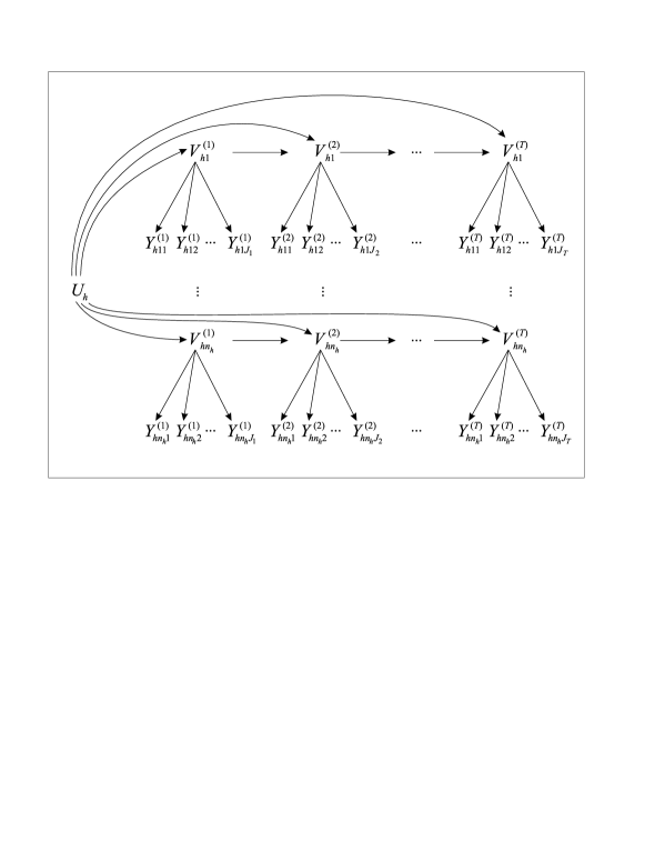
Figure 1: Path diagram representing the multilevel LM model.

The above assumptions lead to a dependence structure between the latent and observable variables which is represented in the path diagram depicted in Figure 1 where, for simplicity, covariates at individual and cluster levels are not indicated explicitly.

In order to complete the model specification, we need to formulate the distribution of the latent variables given the available covariates, which are assumed to be fixed and given. Those covariates may be dummy, categorical or continuous. The covariates referred the $h$-th cluster are collected in the vector $\mbox{\boldmath$x$}_{h}$ and the distribution of $U_{h}$ given these covariates is modeled through the logit parametrization

$$\log\frac{\rho_{h}(u)}{\rho_{h}(1)}=\gamma_{0u}+\mbox{\boldmath$x$}_{h}^{\prime}\mbox{\boldmath$\gamma$}_{1u},\quad u=2,\ldots,k_{1},$$ (3)

where $\rho_{h}(u)=p(U_{h}=u)$ and $\mbox{\boldmath$\gamma$}_{12},\ldots,\mbox{\boldmath$\gamma$}_{1k_{1}}$ are vectors of regression coefficients of the same dimension as $\mbox{\boldmath$x$}_{h}$ and $\gamma_{02},\ldots,\gamma_{0k_{1}}$ are the corresponding intercepts.

The covariates for subject $hi$ at occasion $t$ are denoted by $\mbox{\boldmath$z$}_{hi}^{(t)}$; these covariates are assumed to affect the initial and the transition probabilities of the latent Markov process $V_{hi}^{(1)},\ldots,V_{hi}^{(T)}$ by a parametrization based on global logits. This type of parametrization is also adopted in a similar context by Bartolucci et al. (2008a) and is motivated by the ordinal nature of the variables $V_{hi}^{(t)}$. In particular, for what concerns the initial probabilities

$$\pi_{hi}(v|u)=p(V_{hi}^{(1)}=v|U_{h}=u)$$

we assume

$$\log\frac{\pi_{hi}(v|u)+\cdots+\pi_{hi}(k_{2}|u)}{\pi_{hi}(1|u)+\cdots+\pi_{hi}(v-1|u)}=\delta_{0u}+\delta_{1v}+(\mbox{\boldmath$z$}_{hi}^{(1)})^{\prime}\mbox{\boldmath$\delta$}_{2},\quad u=1,\ldots,k_{1},\quad v=2,\ldots,k_{2},$$ (4)

where $\mbox{\boldmath$\delta$}_{2}$ is a vector of regression parameters of the same dimension as each $\mbox{\boldmath$z$}_{hi}^{(t)}$ which is common to every level $v$; this is an usual assumption of models for ordinal variables based on global logits (McCullagh, 1980). Moreover, the intercepts $\delta_{0u}$ depend on the level of $U_{h}$ and, in order to ensure model identifiability, we let $\delta_{01}\equiv 0$. On the other hand, the intercepts $\delta_{1v}$, depending on the level of $V_{hi}^{(1)}$, must be in decreasing order, i.e. $\delta_{12}\leq\cdots\leq\delta_{1k_{2}}$, to ensure the invertibility of the global logit parametrization.

Finally, as regards the transition probabilities

$$\pi_{hi}^{(t)}(v_{1}|u,v_{0})=p(V_{hi}^{(t)}=v_{1}|U_{h}=u,V_{hi}^{(t-1)}=v_{0})$$

we assume

$$\log\frac{\pi_{hi}^{(t)}(v_{1}|u,v_{0})+\cdots+\pi_{hi}^{(t)}(k_{2}|u,v_{0})}{\pi_{hi}^{(t)}(1|u,v_{0})+\cdots+\pi_{hi}^{(t)}(v_{1}-1|u,v_{0})}=\eta_{0u}^{(t)}+\eta_{1v_{0}v_{1}}^{(t)}+(\mbox{\boldmath$z$}_{hi}^{(t)})^{\prime}\mbox{\boldmath$\eta$}_{2}^{(t)},$$ (5)

with $u=1,\ldots,k_{1}$, $v_{0}=1,\ldots,k_{2}$, $v_{1}=2,\ldots,k_{2}$ and $t=2,\ldots,T$. As above, $\mbox{\boldmath$\eta$}_{2}^{(t)}$ is a common vector of regression coefficients for the individual covariates, the intercepts $\eta_{0u}$ depend on the level of $U_{h}$ (with $\eta_{01}\equiv 0$) and the intercepts $\eta_{0v_{0}v_{1}}$ depend on the levels of $V_{hi}^{(t-1)}$ and $V_{hi}^{(t)}$ and must be decreasing ordered in $v_{1}$ for each $v_{0}$.

Note that the covariates do not have a direct effect on the item responses, but have a direct effect on the distribution the latent variables $U_{h}$ and $V_{hi}^{(t)}$. As such, the support points $\theta_{1},\ldots,\theta_{k_{2}}$ are indeed interpretable as ability levels.

3.3 Interpretation of the parameters

A fundamental issue concerns how to interpret the model parameters. First of all, the model assumes the existence of $k_{2}$ classes of subjects which are ordered according to the ability level. The ability level of class $v$ is denoted by $\theta_{v}$. Moreover, for the $j$-th item administered at the $t$-th occasion, $\beta_{j}^{(t)}$ is the difficulty level measured on the same scale of the ability.

Concerning the interpretation of the parameters for the distribution of the latent variables, it is important to clarify that the intercepts $\delta_{1v}$ and $\eta_{1v_{0}v_{1}}$ in (4) and (5) are relatively less important. Of greater interest are the parameters which characterize the clusters according to their effect on the initial and transition probabilities. In this regard, the model assumes the existences of $k_{1}$ different typologies of clusters. The effect of clusters of type $u$, $u=1,\ldots,k_{1}$, on the initial probabilities is measured by $\delta_{0u}$ and the effect on the transition probability from occasion $t-1$ to occasion $t$ is measured by $\eta_{0u}^{(t)}$. This formulation allows us to consider time varying confounders as well. Those clusters contribute the initial probabilities in (4) and the transition probabilities (5) in a way that it is possible to identify a clear class effect which is time varying.

We can interpret similarly the regression coefficient in the vectors $\mbox{\boldmath$\delta$}_{2}$ and $\mbox{\boldmath$\eta$}_{2}^{(t)}$. With reference to our application, for instance, if we find that $\delta_{02}>\delta_{01}$ and $\eta_{02}^{(2)}<\eta_{01}^{(2)}$, this means that classes of type 2 have a better effect, with respect to classes of type 1, on the ability of their students at the first occasion, but these classes contribute less student’s improvement from the first to the second occasion. Moreover, suppose that for an individual covariate we have a negative coefficient in $\mbox{\boldmath$\delta$}_{2}$, but a positive coefficient in $\mbox{\boldmath$\eta$}_{2}^{(2)}$. Then, as the value of the covariate increases, the ability of the student at the first occasion decreases, but he/she improves more consistently between the first and the second occasion.

Finally, the parameter vectors $\mbox{\boldmath$\gamma$}_{1u}$ in (3) are important for understanding how the distribution of the clusters affects the $k_{2}$ different typologies described above. With reference to our application, suppose that we have three typologies of classes and that for a covariate describing some feature of these classes we have a positive coefficient in both $\mbox{\boldmath$\gamma$}_{12}$ and $\mbox{\boldmath$\gamma$}_{13}$.

This means that, as the value of the covariate increases, there is a greater chance that the class is of type 2 (or of type 3) rather than of type 1. The effect of the covariate on the probability that the class is of type 3 rather than of type 2 depends on the difference between the two regression coefficients. These effects are not always easy to understand and in this case it may convenient to directly consider the probability of each category of $U_{h}$ for different levels of the covariate of interest. This is straightforward when the covariate is a dummy for the class having a particular attribute, such as being in a private rather than public school.

3.4 Computing the manifest distribution

As in Bartolucci and Lupparelli (2007), the manifest distribution of the response variables observed for each cluster $h$ may be expressed as

$$p(\mbox{\boldmath$Y$}_{h}=\mbox{\boldmath$y$}_{h})=\sum_{u}\lambda_{h}(u)\prod_{i}p(\mbox{\boldmath$Y$}_{hi}=\mbox{\boldmath$y$}_{hi}|U_{h}=u),$$ (6)

where $p(\mbox{\boldmath$Y$}_{hi}=\mbox{\boldmath$y$}_{hi}|U_{h}=u)$ may be efficiently computed by a recursion which is known in the literature on hidden-Markov models (Baum et al., 1970, MacDonald and Zucchini, 1997). Details on this recursion are given in Appendix 1.

Finally, the probability $p(\mbox{\boldmath$Y$}_{h}=\mbox{\boldmath$y$}_{h})$ can be easily computed through (6) and the assumption of independence between clusters implies that the manifest distribution of all the response variables is given by

$$p(\mbox{\boldmath$Y$}_{1}=\mbox{\boldmath$y$}_{1},\ldots,\mbox{\boldmath$Y$}_{H}=\mbox{\boldmath$y$}_{H})=\prod_{h}p(\mbox{\boldmath$Y$}_{h}=\mbox{\boldmath$y$}_{h}).$$

4 Likelihood inference

The likelihood of the LM Rasch model may be expressed as

$$\ell(\mbox{\boldmath$\phi$})=\sum_{h}\log p(\mbox{\boldmath$Y$}_{h}=\mbox{\boldmath$y$}_{h}),$$

where $\phi$ is a short-hand notation for all model parameters (see Section 3.2). In this section we show how this function may be maximized, so as to obtain a maximum likelihood estimate of $\phi$ based on the observed sample, and we deal with related inferential problems.

4.1 Estimation

Maximum likelihood estimation of the LM Rasch is carried out on the basis of the EM algorithm (Baum et al., 1970, Dempster et al., 1997). This algorithm is based on the complete data likelihood, i.e. the likelihood that we would compute if we knew the latent state of each subject at each occasion and the value of the latent variable describing the effect of every cluster.

Let $w_{h}(u)$ be a dummy variable equal to 1 if cluster $h$ belongs to latent class $u$, let $z_{hi}^{(t)}(v)$ be a dummy variable equal to 1 if subject $i$ in cluster $h$ is in latent state $v$ at occasion $t$ and let $z_{hi}^{(t)}(v_{0},v_{1})=z_{hi}^{(t-1)}(v_{0})z_{hi}^{(t)}(v_{1})$ be a dummy variable equal to 1 if subject $hi$ moves from state $v_{0}$ to $v_{1}$ at occasion $t$. The complete data log-likelihood may be expressed as

$$\ell^{*}(\mbox{\boldmath$\phi$})=\sum_{h}\sum_{u}w_{h}(u)\{\log[\rho_{h}(u)]+m^{*}_{h}(u)\},$$ (7)

where

$$m_{h}^{*}(u) = \sum_{i}\sum_{v}z_{hi}^{(1)}(v)\log[\pi_{hi}^{(1)}(v|u)]+$$

$$+ \sum_{i}\sum_{v_{0}}\sum_{v_{1}}\sum_{t>1}z_{hi}^{(t)}(v_{0},v_{1})\log[\pi_{hi}^{(t)}(v_{1}|u,v_{0})]+$$

$$+ \sum_{i}\sum_{v}\sum_{t}z_{hi}^{(t)}(v)[y_{hij}^{(t)}\log(\lambda_{j}^{(t)})+(1-y_{hij}^{(t)})\log(1-\lambda_{j}^{(t)})].$$

Since the above dummy variables are not known, the EM algorithm alternates the following two steps until convergence:

• E-step: compute the conditional expected value of the dummy variables $w_{h}(u)$, $z_{hi}^{(t)}(v)$ and $z_{hi}^{(t)}(v_{0},v_{1})$ given the observed data and the current value of the parameters;

• M-step: maximize the conditional expected value of $\ell^{*}(\mbox{\boldmath$\phi$})$ obtained by substituting each dummy variable in (7) with the corresponding expected value obtained from the E-step; the resulting log-likelihood is denoted by $\tilde{\ell}^{*}(\mbox{\boldmath$\phi$})$.

The conditional expected value of $w_{h}(u)$ corresponds to the posterior probability $\tilde{w}_{h}(u)=p(U_{h}=u|\mbox{\boldmath$Y$}_{h}=\mbox{\boldmath$y$}_{h})$ and then, at the E-step, it is computed as

$$\tilde{w}_{h}(u)=\lambda_{h}(u)\prod_{i}p(\mbox{\boldmath$Y$}_{hi}=\mbox{\boldmath$y$}_{hi}|U_{h}=u)/p(\mbox{\boldmath$Y$}_{h}=\mbox{\boldmath$y$}_{h}).$$

Similarly, we have $\tilde{z}_{hi}^{(t)}(v)=p(V_{hi}^{(t)}=v|\mbox{\boldmath$Y$}_{h}=\mbox{\boldmath$y$}_{h})$ and $\tilde{z}_{hi}(v_{0},v_{1})=p(V_{hi}^{(t-1)}=v_{0},V_{hi}^{(t)}=v_{1}|\mbox{\boldmath$Y$}_{h}=\mbox{\boldmath$y$}_{h})$ which are computed as

$$\tilde{z}_{hi}^{(t)}(v) = \sum_{u}\tilde{z}_{hi}^{(t)}(v|u)\tilde{w}_{h}(u),$$

$$\tilde{z}_{hi}^{(t)}(v_{0},v_{1}) = \sum_{u}\tilde{z}_{hi}^{(t)}(v_{0},v_{1}|u)\tilde{w}_{h}(u),$$

where the conditional probabilities

$$\tilde{z}_{hi}^{(t)}(v|u) = p(V_{hi}^{(t)}=v|U_{h}=u,\mbox{\boldmath$Y$}_{h}=\mbox{\boldmath$y$}_{h})$$

$$\tilde{z}_{hi}^{(t)}(v_{0},v_{1}|u) = p(V_{hi}^{(t-1)}=v_{0},V_{hi}^{(t)}=v_{1}|U_{h}=u,\mbox{\boldmath$Y$}_{h}=\mbox{\boldmath$y$}_{h})$$

may be obtained by certain recursions which are illustrated in Appendix 2.

Finally, the M-step is based on standard iterative algorithms to maximize each component of $\tilde{\ell}^{*}(\mbox{\boldmath$\phi$})$. These algorithms are the same as those used to estimate a multinomial logit model on the basis of a weighted log-likelihood.

It is important to mention that, as typically happens for latent variable models, the likelihood of the proposed model may be multimodal and has a number of local maxima which increases with the number of latent variables and that of the states. It is thus crucial to choose the initial values of the EM algorithm appropriately. In particular, we select the intercepts corresponding to the different levels of the latent variables $U_{h}$ and $V_{hi}^{(t)}$ on a grid of, respectively, $k_{1}$ and $k_{2}$ equispaced points around 0. Moreover, all the regression coefficients for the covariates are fixed at 0, whereas the difficulty levels of the items are chosen on the basis of the observed frequencies of correct responses.

4.2 Model selection and hypothesis testing

For model selection, we rely on the Bayesian Information Criterion (BIC; Schwarz, 1978), which is based on the index

$$BIC=-2\ell(\hat{\mbox{\boldmath$\phi$}})+r\log(n),$$

where $\ell(\hat{\mbox{\boldmath$\phi$}})$ is the maximum log-likelihood of the model of interest and $r$ is the number of parameters; the latter obviously depends on both $k_{1}$ and $k_{2}$. According to this criterion, the optimal combination of $k_{1}$ and $k_{2}$ is the one corresponding to the model with the smallest BIC value.

For testing a hypothesis on the parameters, we rely on the likelihood ratio statistic $D=-2[\ell(\hat{\mbox{\boldmath$\phi$}}_{0})-\ell(\hat{\mbox{\boldmath$\phi$}})]$, where $\hat{\mbox{\boldmath$\phi$}}_{0}$ is the estimate of the parameter vector under the hypothesis of interest, which can be computed through the same EM algorithm described in section 4.1. To compute the standard errors for the parameter estimates we rely on a method similar to the likelihood profiling method (Meeker and Escobar, 1995). In particular, for the estimate $\hat{\phi}_{h}$ of the parameter $\phi_{h}$, we first compute the likelihood ratio statistic $D_{h}$ for testing the hypothesis $H_{0}:\phi_{h}=0$ and then we compute the standard error $se(\hat{\phi}_{h})$ as $|\hat{\phi}_{h}|/\sqrt{D_{h}}$. In this way, the conclusion of the Wald test for $H_{0}$ based on the statistic $\hat{\phi}_{h}/se(\hat{\phi}_{h})$ is guaranteed to be the same as the test based on the statistic $D_{h}$.

5 Application to the Lombardy dataset

We now illustrate the analysis of the longitudinal patterns of achievement levels in Mathematics measured by the tests administrated at the end of each school year between the two subgroups of students attending public and paritarie schools.

Table 1 presents the frequency distribution of the available characteristics of the public and paritarie middle schools in 2003 at population level on the selected areas of Lombardy. Table 2 shows the corresponding sample distributions, including a dummy variable related to the years since school opened. It can be seen that the sample and the population distributions look similar for both types of school. In both cases, the public schools enroll more students and have a higher student-teacher ratio. Table 3 concerns the social background characteristics of the students. It reports the percentage values of father and mother level of education and the percentage of missing responses.

5.1 Model fitting and Results

We here report the results obtained by applying the multilevel Rasch LM model to the available dataset. We fitted the proposed model including the students and the school covariates. We also included two dummy variables to account for the student missing responses on the questions related to father and mother levels of education.

We fitted the model for a different number of latent states at cluster level ($k_{1}$), ranging form 1 to 5, and individual level ($k_{2}$), ranging from 1 to 7. Table 4 shows the results of the fitted models reporting the maximum log-likelihood $(\hat{\ell}_{k_{1},k_{2}})$ of the estimated model, the value attained by the BIC index and the number of parameters. We observe that the lowest value of the BIC index corresponds to four typologies of clusters ($k_{1}=4$) and six math ability levels ($k_{1}=6$). We then identify six subgroups of students with different levels of ability and four different types of school classes.

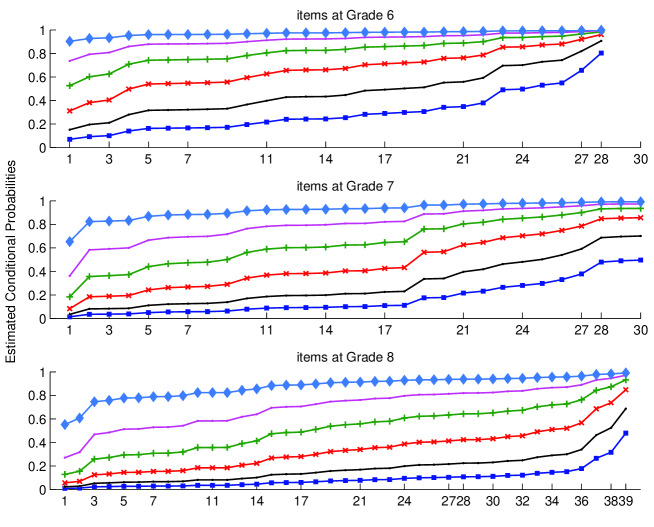
Figure 2: Ordered estimated conditional probabilities for latent classes 1-5: blue square, class 1; black bullet class 2; red times, class 3; green plus, class 4; pink bullet, class 5; heavenly diamond, class 6. The first graph form the top is referred to the items administrated at Grade 6, the second at Grade 7 and the third at Grade 8.

The estimated abilities for each latent state are reported in Table 5. These abilities range from the lowest to the highest levels; note that the ability of the first class is constrained to be 0 to guarantee identifiability. These results are in accordance with the six student proficiency levels in Mathematics identified in the OCSE-PISA reports (see for example OECD, 2007). They may represent some specific types of task in math that a student is likely to perform successfully. A better interpretation of these latent classes can be gained by looking at the estimated conditional probabilities parameterized through a logit function of the abilities and of the item difficulties. They are depicted in Figure 2 for each level of ability and according to the different item which has been administrated at each grade. From this figure we can read the probability of responding correctly to each set of items for each grade for a student belonging to one of the six latent classes. They are ordered from the lowest to the highest in each graph.

As we would expect, these probabilities are higher for the items administrated at Grade 6 (top-most graph) and are lower for the items administrated at Grade 8 (bottom graph). It means that the difficulty of the items is increasing over time. The items which have been replicated over time share the same value of those probabilities. For example item number 2 on the top graph is replicated at Grade 7 and it corresponds to item number 13 of middle graph. Additional observations can be drawn from this figure. For example the probability of responding correctly to the items administered at Grade 6 ranges between 0.8 and 1 for the students with the highest ability. It ranges, instead, between 0 and 0.8 for the students with the lowest ability level. This means that they are specially tailored to measures the abilities of the less capable students.

Table 6 displays the estimates of the intercepts and the regression coefficients for the logistic model at cluster level, which is based on parametrization (3). There are three ordered intercepts, one for each of the three clusters identified by the letters B, C and D. The equality restrictions to zero have been imposed on the parameters of the first latent class (A) to make the model identifiable. The other estimated parameters are the regression coefficients for the covariate type of school labeled with 1, to the ratio between students and teachers labeled with 2, and to the dummy variable indicating the years of activity of the school labeled with 3. As the value of the covariate ratio between student and teachers increases, there is less chance that the class is of type A rather than of type B. On the other hand, as the value of the years of activity of the school increases there is more chance that the class is of type A rather than of type B.

To better interpret these estimates, it is convenient to consider the probability of each cluster for different levels of the covariate of interest. For example the average class probability of belonging to each cluster is reported in Table 7. It indicates that 78% of the classes of the paritarie schools belong to cluster A and 23% to cluster D, whereas the percentage is 32% and 6% for the classes of the public middle schools. On the basis on these results we conclude that the classes of type A are prevalently those of paritarie schools with small values of the ratio between students and teachers and with years of activity higher than eighteen. The classes of type B are mainly in public schools with different years of activity and values of the ratio between students and teachers higher than eight. The classes of type C are mainly in public schools with different values of years of activity and of the ratio between students and teachers. The classes of type D are mainly in paritarie schools with years of activity less than eighteen and with low values of the ratio between students and teachers.

Table 8 displays the estimates of the intercepts and the regression coefficients for the initial probabilities of the latent Markov process. These parameter estimates can be interpreted on the basis of formula (4). In particular, there are three ordered intercepts corresponding to the effect on the initial probability of the clusters B, C and D. Therefore the classes of type B help less to increase the math ability on the first year of the middle school compared to the classes of the other clusters. The classes helping more on the first year are those of type C.

Table 9 shows the effects of the same variables on the transition probabilities, from Grade 6 to 7 and Grade 7 to 8, of the latent Markov process. On the basis of the estimated coefficients we can state that the classes of type B contribute less on the math ability of their students than those of type C and the classes of type D have a high positive effect on the math ability from Grade 6 to Grade 7. However if we consider the estimated coefficients related to the transition form Grade 7 to 8, type C classes contribute the most to students’ math ability.

Looking at the estimated regression coefficients related to the covariate level of education of the father we can see that the ability of the students increases for those having higher educated fathers. The magnitude of this increase is less strong than on Grade 6 and is quite the same for the transition form Grade 6 to 7 and from Grade 7 to 8. For the global logit on the transition probablities from Grade 7 to 8 the variables related to the missing values are significant as well. On the basis of the estimates in Table 9 we conclude that the contribution of the level of education of the father is always inferior of the contribution of type of class on the math achievement.

Finally, we provide a comparison of the above results with some descriptive statistics on the student’s scores of the sample across grades. In particular, Table 10 and Table 11 report, for public and paritarie middle schools, the empirical transition matrices obtained by dividing the sum of the scores for each subject in each grade into six classes of score. Looking at these probabilities from Grade 6 to Grade 7 and from Grade 7 to Grade 8 for both types of schools it can be noticed that the students do not improve their abilities as much as we might expect. There is not a transition towards state characterizing higher scores but there is great persistence in the same state. This is also true for the transition from Grade 7 to Grade 8 for both types of schools. For both the paritarie and public schools, students with less ability have some chance of becoming better performers at the end of the middle school. Individuals attending public schools who are in the first knowledge state show a probability of 0.67 of moving to a better knowledge state form Grade 6 to Grade 7 and a probability of 0.35 of moving from state 2 at Grade 7 to state 3 at Grade 8. In the paritarie schools there are more students with the highest ability level at Grade 8 compared to the public schools. The empirical transition matrices seem to have a tridiagonal structure: the transition is possible only below or above the diagonal.

6 Conclusions

We propose a multilevel extension of the LM Rasch model for the analysis of longitudinal data derived from the repeated administration of binary test items to students attending public and private middle schools in the Lombardy Region of Italy. The items are aimed at assessing math knowledge of the students during the three years of middle school. Taking into account that student actual knowledge and the potential to increase such knowledge depends on prior knowledge and socio-cognitive aspects, such as family and school, we propose an alternative method to growth models.

We show how the multilevel extension of the LM Rasch model allows us to make a comparison between two types of schools with different pupil achievement. The model assumes the existence of a latent Markov chain for the ability level dynamics and it allows us to model the probability of individual changes over time, while taking into account the hierarchical structure of the data. It allows us to flexibly parameterize the conditional distribution of the vector of the response variables in order to take into account the different number of items administered at each grade and the fact that items may be replicated at different occasions.

We have shown that the acquisition of mathematical knowledge is a result of the differences between student’s background and personal behavior. Moreover the rate of change that brings the student from one knowledge level to the following one may also depend on the quality of the school. When the school tends to its task, family background is less influential on student results. Therefore we could also conclude that the lower the parental education is, the more the school helps.

Our results demonstrate that the model on which our approach is based can describe the main relationships in the data with a rather parsimonious structure. Moreover it takes into account that cognitive achievement changes over time in relation to the background variables of the student and the class type.

A causal interpretation can be given to the estimated regression coefficients as the school covariates appear to have the same distribution on the population of the school in Lombardy. Obviously, in drawing conclusions on the basis of the application we have to consider that schools participate on a voluntary basis in the IRRE project from which the available data have been collected. This could have determined a selection bias. For instance, it is possible that the choice to participate in the study was only made by the best organized schools with the most qualified teachers.

Appendices

Appendix 1: computing manifest probabilities

Following Bartolucci (2006) and Bartolucci et al. (2007), we describe the recursion to compute $p(\mbox{\boldmath$Y$}_{hi}=\mbox{\boldmath$y$}_{hi}|U_{h}=u)$ by using the matrix notation. This makes its implementation easier in most mathematical and statistical packages.

Let $\mbox{\boldmath$p$}_{hi}^{(t)}$ be a column vector with elements

$$p(\mbox{\boldmath$Y$}_{hi}^{(t)}=\mbox{\boldmath$y$}_{hi}^{(t)}|V_{hi}^{(t)}=v) = \prod_{j}p(Y_{hij}^{(t)}=y_{hij}^{(t)}|V_{hi}^{(t)}=v)=$$

$$= \prod_{j}[\lambda_{j}^{(t)}]^{y_{hij}^{(t)}}[1-\lambda_{j}^{(t)}]^{1-y_{hij}^{(t)}},\quad v=1,\ldots,k_{2},$$

and consider the vector $\mbox{\boldmath$q$}_{hi}^{(t)}(u)$ with elements

$$p(\mbox{\boldmath$Y$}_{hi}^{(1)}=\mbox{\boldmath$y$}_{hi}^{(1)},\ldots,\mbox{\boldmath$Y$}_{hi}^{(t)}=\mbox{\boldmath$y$}_{hi}^{(t)}|U_{h}=u,V_{hi}^{(t)}=v),\quad v=1,\ldots,k_{2}.$$

The recursion mentioned above allows us to compute this vector as

$$\mbox{\boldmath$q$}_{it}(u)=\left\{\begin{array}[]{ll}\textrm{diag}(\mbox{\boldmath$p$}_{hi}^{(1)})\mbox{\boldmath$\pi$}_{hi}(u)&\mbox{ for }t=1,\\ \textrm{diag}(\mbox{\boldmath$p$}_{hi}^{(t)})[\mbox{\boldmath$\Pi$}_{hi}^{(t)}(u)]^{\prime}\mbox{\boldmath$q$}_{i,t-1}(u)&\mbox{ for }t=2,\ldots,T,\\ \end{array}\right.$$

where the vector $\mbox{\boldmath$\pi$}_{hi}(u)$ has elements $\pi_{hi}(v|u)$, $v=1,\ldots,k_{2}$, and the matrix $\mbox{\boldmath$\Pi$}_{hi}^{(t)}(u)$ has elements $\pi_{hi}^{(t)}(v_{1}|u,v_{0})$, $v_{0},v_{1}=1,\ldots,k_{2}$. At the end of the recursion, we obtain $\mbox{\boldmath$q$}_{iT}(u)$; the sum of the elements of this vector is equal to $p(\mbox{\boldmath$Y$}_{hi}=\mbox{\boldmath$y$}_{hi}|U_{h}=u)$.

Appendix 2: computing posterior probabilities

Let $\mbox{\boldmath$z$}^{(t)}_{hi}(u)$ be the column vector with elements $\tilde{z}_{hi}^{(t)}(v|u)$, $v=1,\ldots,k_{2}$, and and $\mbox{\boldmath$Z$}^{(t)}_{hi}(u)$ be the matrix with elements $\tilde{z}_{hi}^{(t)}(v_{0},v_{1}|u)$, $v_{0},v_{1}=1,\ldots,k_{2}$. These may be computed through the following backward recursion (see Levinson et al., 1983, and MacDonald and Zucchini, 1997, Bartolucci et al., 2007):

$$\mbox{\boldmath$z$}^{(t)}_{hi}(u) = {\rm diag}[\mbox{\boldmath$q$}_{hi}^{(t)}(u)]\mbox{\boldmath$r$}_{hi}^{(t)}/p(\mbox{\boldmath$Y$}_{hi}=\mbox{\boldmath$y$}_{hi}|U_{h}=u),$$

$$\mbox{\boldmath$Z$}^{(t)}_{hi}(u) = {\rm diag}[\mbox{\boldmath$q$}_{hi}^{(t-1)}(u)]\mbox{\boldmath$\Pi$}_{hi}^{(t)}(u){\rm diag}(\mbox{\boldmath$p$}_{hi}^{(t)})\textrm{diag}(\mbox{\boldmath$r$}_{hi}^{(t)})/p(\mbox{\boldmath$Y$}_{hi}=\mbox{\boldmath$y$}_{hi}|U_{h}=u),$$

where

$$\mbox{\boldmath$r$}_{hi}^{(t)}(u)=\left\{\begin{array}[]{ll}\mbox{\boldmath$1$}_{k_{2}}&\mbox{ if }t=T,\\ \mbox{\boldmath$\Pi$}^{(t+1)}\textrm{diag}[\mbox{\boldmath$p$}_{hi}^{(t+1)}(u)]\mbox{\boldmath$r$}_{hi}^{(t+1)}(u)&\mbox{ otherwise},\end{array}\right.$$

with $\mbox{\boldmath$1$}_{k_{2}}$ denoting a column vector of $k_{2}$ ones.

References

Bartolucci, F. (2006). Likelihood inference for a class of latent Markov models under linear hypotheses on the transition probabilities. Journal of the Royal Statistical Society, series B, 68, 155–178.

Bartolucci, F. and Lupparelli, M. (2007). The multilevel latent Markov model. Proceedings of the International Workshop on Statistical Modelling, Barcelona, July 2007, pp. 93-98.

Bartolucci, F., Lupparelli, M. and Montanari, G. E. (2008a), Latent Markov model for binary longitudinal data: an application to the performance evaluation of nursing homes, to appear in Annals of Applied Statistics, available at www.stat.unipg.it\bartolucci\.

Bartolucci, F. and Pennoni, F. (2007). A class of latent Markov models for capture-recapture data allowing for time, heterogeneity, and behavior effects. Biometrics, 63, 568–568.

Bartolucci, F., Pennoni, F. and Francis, B. (2007). A latent Markov model for detecting patterns of criminal activity. Journal of the Royal Statistical Society, series A, 170, 115–132.

Bartolucci, F., Pennoni, F., Lupparelli, M. (2008b). Likelihood inference for the latent Markov Rasch model. In: C. Huber, N. Limnios, M. Mesbah, M. Nikulin (Eds.), Mathematical Methods for Survival Analysis, Reliability and Quality of Life, 239–254, Wiley.

Baum, L. E., Petrie, T., Soules, G. and Weiss, N. (1970), A maximization technique occurring in the statistical analysis of probabilistic functions of Markov chains, Annals of Mathematical Statistics, 41, pp. 164-171.

Dronkers J. and Robert P. (2008). Differences in Scholastic Achievement of Public, Private Government-Dependent, and Private Independent Schools. Educational Policy 22, 541-577.

Goldstein H., Bonnet G. and Rocher T. (2007). Multilevel Structural Equation Models for the Analysis of Comparative Data on Educational Performance. Journal of Educational and Behavioral Statistics, 32, 252-286.

Dempster, A. P., Laird, N. M. and Rubin, D. B. (1977). Maximum likelihood from incomplete data via the EM algorithm (with discussion). J. R. Statist. Soc. series B, 39, 1-38.

Hong G. and Raudenbush S. W. (2008). Causal Inference for Time-Varying Instructional Treatments. Journal of Educational and Behavioral Statistics, 33, 333-362.

Langeheine, R. and van de Pol, F. (2002), Latent Markov Chains, in Advances in Latent Class Analysis, A. L. McCutcheon and J. A. Hagenaars editors, University Press, Cambridge.

Levinson, S. E., Rabiner, L. R. and Sondhi, M. M. (1983), An introduction to the application of the theory of probabilistic functions of a Markov process to automatic speech recognition, Bell System Technical Journal, 62, pp. 1035-1074.

Lubienski, S.T. and Lubienski, C. (2006). School sector and academic achievement: A multi-level analysis of NAEP mathematics data. American Educational Research Journal, 43, 651-698.

Lubienski, C., Crane, C. C. and Lubienski, S. T. (2008). What Do We Know About School Effectiveness? Academic Gains in a Value-Added Analysis of Public and Private Schools. Phi Delta Kappan, 89, 689-695.

McCullagh, P. (1980). Regression models for ordinal data (with discussion). Journal of the Royal Statistical Society, series B, 42, 109-142.

MacDonald, I. and Zucchini, W. (1997). Hidden Markov and Other Models for Discrete-valued Time Series. London: Chapman & Hall.

Meeker, W. Q. and Escobar L. A. (1995). Teaching about approximate confidence regions based on maximum likelihood estimation. American Statistician, 49,1, 48-53.

McEwan P. J. (2000). The Potential Impact of Large-Scale Voucher Programs. Review of Educational Research, 70, 103-149.

Morgan S. L. and Winship C. (2007). Counterfactual and Causal inference. Methods and Principles for Social Research. Cambridge University Press.

National Assessment of Educational Progress (2005). The Nation’s Report Card Student Achievement in Private Schools. United States Department of Education, Institute of Education Sciences NCES 2006-459.

National Assessment of Educational Progress (2006). Comparing Private Schools and Public Schools Using Hierarchical Linear Modeling. United States Department of Education, Institute of Education Sciences NCES 2006-461.

OECD (2007). Executive Summary PISA (2006): Science Competencies for Tomorrow s World. OECD report. Available at
http://www.oecd.org/dataoecd/15/13/39725224.pdf.

Rasch, G. (1961). On general laws and the meaning of measurement in psychology. Proceedings of the IV Berkeley Symposium on Mathematical Statistics and Probability, 4, 321-333.

Raudenbush, S.W. and Bryk A. (2002). Hierarchical Linear Models: Applications and Data Analysis Methods.(Second edition), Newbury Park, CA: Sage Publications.

Rubin, D.B., Stuart, E.A. and Zanutto, E.L. (2004). A potential outcomes view of value-added assessment in education. Journal of Educational and Behavioral Statistics, 29, Value-Added Assessment Special Issue, pp. 103-116.

Schneider B., Carnoy M., Kilpatrick J., Schmidt W. H. and Shavelson R. J. (2007). Estimating Causal Effects Using Experimental and Observational Designs. A Think Tank White Paper, Washington Dc: American Educational Research Association.

Schwarz, G. (1978). Estimating the dimension of a model, Annals of Statistics, 6, 461-464.

Snijders, T.A.B. and Bosker, R. J. (1999). Multilevl Analysis. London: Sage Publications.

Stuart E. A. (2007). Estimating Causal Effects Using School-Level Data Sets. Educational Researcher, 36, 187-198.

Vermunt, J. K. Langeheine, R., B ckenholt, U. (1999). Discrete-time discrete state latent Markov models with time-constant and time-varying covariates. Journal of Educational and Behavioral Statistics, 24, 178-205.

Wiggins, L. M. (1973). Panel Analysis: Latent Probability Models for Attitudes and Behavior Processes. Amsterdam: Elsevier

		$public$		$paritarie$
		$\%$	cum $\%$	$\%$	cum$\%$
number of students
	(0-200)	49.02	49.02	82.59	82.59
	(200-350)	31.30	80.31	17.41	100.00
	(350-700)	15.55	95.87	00.00	100.00
	(700-1050)	4.13	100.00	00.00	100.00
number of teachers
	(0-20)	20.90	20.90	53.86	53.86
	(20-40)	32.52	53.42	46.14	100.00
	(40-70)	30.63	84.05	00.00	100.00
	(70-105)	15.95	100.00	00.00	100.00
students-teachers ratio
	(1-6)	6.50	6.50	11.13	11.13
	(6-8)	22.05	28.54	25.12	36.25
	(8-12)	64.17	92.72	17.20	53.45
	(12-20)	7.28	100.00	45.55	100.00

Table 1: Frequency distributions of the number of students and teachers and their ratio at the school level for the public and paritarie middle schools in the selected areas.

		$public$		$paritarie$
		$\%$	cum $\%$	$\%$	cum$\%$
number of students
	(0-200)	15.38	15.38	85.71	85.71
	(200-350)	30.77	46.15	14.29	100.00
	(350-700)	30.77	76.92	0.000	100.00
	(700-1050)	23.08	100.00	0.000	100.00
number of teachers
	(0-20)	15.38	15.38	57.14	57.14
	(20-40)	30.77	46.15	42.86	42.86
	(40-70)	38.46	84.62	0.000	0.000
	(70-105)	15.38	100.00	0.000	0.000
students-teachers ratio
	(1-6)	0.000	0.000	14.29	14.29
	(6-8)	30.77	30.77	28.57	42.86
	(8-12)	61.54	92.31	14.29	57.14
	(12-20)	7.69	100	42.86	100.00
years since school opened
	$\leq 17.5$	69.20	69.20	71.40	71.40
	$>17.5$	30.80	100.00	28.60	100.00

Table 2: Frequency distributions of the number of students, teachers and their ratio and the years the school has been in operation for the public and paritarie middle schools included in the observed sample.

		$public$	$paritarie$
		$\%$	$\%$	total
Father’s education
	no response	7.34	14.29	8.75
	primary school	3.92	1.59	3.45
	middle school	25.96	9.13	22.25
	high school	38.93	35.71	38.28
	college degree or higher	23.84	39.29	26.97
Mother’s education
	no response	6.64	12.30	57.14
	primary school	3.62	0.79	3.05
	middle school	25.75	9.52	22.47
	high school	44.06	40.87	43.42
	college degree or higher	19.92	36.51	23.27

Table 3: Frequency distribution of parental education of public and paritarie middle school students included in the sample.

$k_{1}$	$k_{2}$	$\hat{\ell}_{k_{1},k_{2}}$	$BIC_{k_{1},k_{2}}$	$np$
1	1	-76565.77	153737.40	85
1	2	-71340.91	143415.97	103
1	3	-70275.94	141357.31	113
1	4	-69878.97	140663.16	127
1	5	-69703.14	140439.79	145
1	6	-69703.14	140439.79	145
1	7	-69561.12	140497.88	193
2	2	-71266.31	143316.67	110
2	3	-70187.30	141229.93	120
2	4	-69771.10	140497.30	134
2	5	-69579.94	140243.28	152
2	6	-69490.77	140221.77	174
2	7	-69425.48	140276.51	200
3	2	-70187.30	141229.93	120
3	3	-70128.67	141162.56	127
3	4	-69707.65	140420.31	141
3	5	-69515.20	140163.70	159
3	6	-69410.43	140110.98	181
3	7	-69349.18	140173.78	207
4	2	-71204.06	143291.96	124
4	3	-70093.64	141142.39	134
4	4	-69664.37	140383.63	148
4	5	-69482.37	140147.94	166
4	6	-69374.80	140089.61	188
4	7	-69315.71	140156.75	214
5	2	-71184.70	143303.13	131
5	3	-70073.61	141152.23	141
5	4	-69631.02	140366.83	155
5	5	-69457.00	140147.09	173
5	6	-69356.58	140103.06	195
5	7	-69297.09	140169.39	221

Table 4: For any number of latent states at cluster level ($k_{1}$) and at individual level ($k_{2}$), $\hat{\ell}_{k_{1},k_{2}}$ is the corresponding maximum log-likelihood, $BIC_{k_{1},k_{2}}$ is the corresponding BIC index and $np$ the number of parameters. Figures in boldface correspond to the model with the smallest value of the BIC index.

$v$	$\theta_{v}$
1	$0.000$
2	$0.866$
3	$1.800$
4	$2.698$
5	$3.623$
6	$4.825$

Table 5: Estimated math ability levels across all groups of students.

		estimates	s.e.	$p-value$
	$\gamma_{0C}$	-42.030	-	-
	$\gamma_{1B1}$	28.815	17.481	0.099
	$\gamma_{1B2}$	1.263	0.417	0.002
	$\gamma_{1B3}$	-1.283	1.007	0.203
	$\gamma_{0C}$	-31.359	-	-
	$\gamma_{1C1}$	28.389	10.144	0.005
	$\gamma_{1C2}$	0.336	0.231	0.145
	$\gamma_{1C3}$	-0.574	0.973	0.555
	$\gamma_{0D}$	2.851	-	-
	$\gamma_{1D1}$	-0.039	0.967	0.968
	$\gamma_{1D2}$	-0.620	0.221	0.005
	$\gamma_{1D3}$	2.754	1.154	0.017

Table 6: Estimated intercepts and regression coefficients of the logit defined on the group level latent variable for the covariate type of school labeled with 1 (public or paritaria), the ratio between students and teachers labeled with 2 and for the dummy variable years since school opened labeled with 3 for any number of group level latent class $u=A,B,C,D$.

	$A$	$B$	$C$	$D$
public	0.325	0.233	0.376	0.066
paritarie	0.786	0.000	0.000	0.214
$\geq 17.5$ years	0.425	0.189	0.314	0.072
$<17.5$ years	0.363	0.196	0.289	0.152
$<8$	0.541	0.090	0.205	0.164
$\geq 8$	0.337	0.245	0.363	0.054

Table 7: Average class probabilities among type of school, years since school opened and ratio between students and teachers of belonging to each latent class of the group latent variable $U$.

		estimates	s.e	$p$-value
	$\delta_{0B}$	- 0.261	-	-
	$\delta_{0C}$	1.140	-	-
	$\delta_{0D}$	0.013	-	-
	$\delta_{2,mF}$	1.058	3.273	0.747
	$\delta_{2,F}$	0.403	0.143	0.005
	$\delta_{2,mM}$	0.139	0.054	0.011
	$\delta_{2,M}$	0.292	0.067	0.000

Table 8: Estimated intercepts for each cluster level of the global logit defined on the initial probabilities. Estimated regression parameters common for each ability level for the covariate father’s education labeled with F and mother’s education labeled with M and for the dummy variable for missing responses labeled with mF and mM respectively.

		estimates	s.e	$p$-value
	$\eta_{0B}^{2}$	-2.774	-	-
	$\eta_{0C}^{2}$	-0.317	-	-
	$\eta_{0D}^{2}$	4.515	-	-
	$\eta_{0B}^{3}$	3.893	-	-
	$\eta_{0C}^{3}$	1.673	-	-
	$\eta_{0D}^{3}$	-0.434	-	-
	$\eta_{2,mF}^{2}$	-0.675	0.349	0.053
	$\eta_{2,F}^{2}$	0.281	0.141	0.046
	$\eta_{2,mM}^{2}$	0.581	0.670	0.386
	$\eta_{2,M}^{2}$	0.007	0.164	0.965
	$\eta_{2,mF}^{3}$	0.867	0.414	0.036
	$\eta_{2,F}^{3}$	0.320	0.125	0.011
	$\eta_{2,mM}^{3}$	0.765	0.135	0.015
	$\eta_{2,M}^{3}$	0.143	0.172	0.406

Table 9: Estimated parameters affecting the transition probabilities from Grade 6 to 7 (2) and Grade 7 to 8 (3) of the latent Markov process. Estimated effects of the clusters and estimated regression coefficients of the variables father’s and mother’s education labeled with F and M respectively and of the dummy variable for the missing responses labeled with mF and mM respectively

	$Grade$ $7$
$Grade$ $6$	$1$	$2$	$3$	$4$	$5$	$6$	$total$
1	0.11	0.67	$0.22$	$0.00$	$0.00$	0.02	1.00
2	$0.05$	0.36	0.37	$0.16$	$0.06$	0.00	1.00
3	0.02	$0.21$	0.44	$0.23$	$0.07$	0.02	1.00
4	0.00	$0.09$	0.27	0.35	$0.24$	0.04	1.00
5	$0.00$	0.02	0.19	0.31	0.35	0.14	1.00
6	$0.01$	0.02	0.04	0.15	0.40	0.35	1.00

	$Grade$ $8$
$Grade$ $7$	$1$	$2$	$3$	$4$	$5$	6	$total$
1	0.00	0.53	$0.18$	$0.06$	$0.06$	0.18	1.00
2	0.03	0.38	0.35	$0.21$	$0.02$	0.01	1.00
3	0.01	0.22	0.30	0.32	$0.13$	0.03	1.00
4	0.00	0.07	0.24	0.42	$0.23$	0.05	1.00
5	0.00	0.01	0.04	0.23	0.30	0.14	1.00
6	0.00	0.03	0.17	0.35	0.44	0.00	1.00

Table 10: Empirical transition probabilities from Grade 6 to Grade 7 and from Grade 7 to Grade 8 for students attending public school. Figures in italic and boldface correspond to the largest probability in any row.

	$Grade$ $7$
$Grade$ $6$	$1$	$2$	$3$	$4$	$5$	$6$	$total$
1	0.00	0.33	0.67	$0.00$	$0.00$	0.00	1.00
2	0.03	0.26	0.28	0.28	$0.13$	0.03	1.00
3	0.02	0.11	0.41	0.27	$0.12$	0.08	1.00
4	0.00	0.02	0.26	0.38	$0.24$	0.11	1.00
5	$0.00$	0.02	0.30	0.45	0.23	0.00	1.00
6	$0.00$	0.00	0.00	0.00	0.43	0.57	1.00

	$Grade$ $8$
$Grade$ $7$	$1$	$2$	$3$	$4$	$5$	6	$total$
1	0.50	0.50	$0.00$	$0.00$	0.00	0.00	1.00
2	0.10	0.60	0.30	$0.00$	$0.00$	0.00	1.00
3	0.00	0.25	0.45	$0.28$	$0.03$	0.00	1.00
4	0.00	0.03	0.27	0.51	$0.19$	0.00	1.00
5	0.00	0.02	0.05	0.26	0.53	0.14	1.00
6	0.00	0.00	0.00	0.07	0.17	0.28	1.00

Table 11: Empirical transition probabilities from Grade 6 to Grade 7 and from Grade 7 to Grade 8 for students attending paritaria school. Figures in italic and boldface correspond to the largest probability in any row.