Search for three-nucleon force effects
on the longitudinal response function of ⁴He

Abstract

A detailed study of the ⁴He longitudinal response function $R_{L}(\omega,q)$ is performed at different kinematics, with particular emphasis on the role of three-nucleon forces. The effects shown are the results of an ab initio calculation where the full four-body continuum dynamics is considered via the Lorentz integral transform method. The contributions of the various multipoles to the longitudinal response function are analyzed and integral properties of the response are discussed in addition. The Argonne V18 nucleon-nucleon interaction and two different three-nucleon force models (Urbana IX, Tucson-Melbourne^′) are used. At lower momentum transfer ($q\leq 200$ MeV/c) three-nucleon forces play an important role. One even finds a dependence of $R_{L}$ on the three-nucleon force model itself with differences up to 10%. Thus a Rosenbluth separation of the inclusive electron scattering cross section of ⁴He at low momentum transfer would be of high value in view of a discrimination between different three-nucleon force models.

I Introduction

An aspect of nuclear dynamics that has attracted a lot of interest in the last years is the importance of multi-nucleon forces and in particular of the three-nucleon force (3NF). The nuclear potential has clearly an effective nature, therefore it is in principle a many-body operator. Yet the debate has concentrated for several decades mainly on its two-nucleon part. Such a debate has taken place among the advocates of three different approaches based on meson theory, pure phenomenology and more recently effective field theory. Realistic potentials have been obtained within the three different frameworks, relying on fits to thousands of N-N scattering data. As is well known such realistic potentials do not explain the triton binding energy and thus 3NF are necessary. Today, due to effective field theory approaches a new debate is taking place regarding 3NF. However, for the determination of a realistic three-body potential or to discriminate among different models one needs to find A$\geq 3$ observables that are 3NF sensitive. An important activity in this direction has taken place in the last years, with accurate calculations of bound-state properties of nuclei of increasing mass number A Pieper02 ; Navratil07 .

We follow a complementary approach and direct our attention, instead, towards electromagnetic reactions in the continuum. In fact many years of electron scattering experiments have demonstrated the power of electro-nuclear reactions, and in particular of the inelastic ones, in providing important information on nuclear dynamics. The possibility to vary energy $\omega$ and momentum $q$ transferred by the electron to the nucleus allows one to focus on different dynamical aspects. In fact one might find regions where the searched three-nucleon effects are sizable. The choice of the ⁴He target is particularly appropriate because of the following considerations. i) The ratio between the number of triplets and of pairs goes like (A-2)/3, therefore doubles from ³He to ⁴He. ii) Theoretical results on hadronic scattering observables involving four nucleons have already shown that three-body effects are rather large Kievsky08 ; Deltuva08 . iii) Since ⁴He has quite a large average density and its binding energy per particle is similar to that of heavier systems, it can serve as a guideline to investigate heavier nuclei. iv) Various inclusive ⁴He $(e,e^{\prime})$ experiments have already been performed in the past Carlson02 , where Rosenbluth separations have been carried out. Due to the low atomic number it is possible to study the longitudinal and the transverse responses separately, without the ambiguities created by the Coulomb distortions affecting heavier systems. v) The Lorentz Integral Transform (LIT) method EFROS94 ; REPORT07 allows to extend investigations beyond the three- and four-body break up thresholds.

In this work we concentrate on the longitudinal response function $R_{L}(\omega,q)$ at constant momentum transfers $q\leq$ 500 MeV/c. Since the longitudinal response $R_{L}$ is much less sensitive to meson exchange effects than the transverse response $R_{T}$ the use of a simple one-body density operator allows to concentrate on the nuclear dynamics generated by the potential. In fact, for low $q$ two-body operators in $R_{L}$ are only of fourth order in effective field theory counting (N³LO) PARK03 , and their contribution is negligible up to $q\approx$ 300 MeV/c, see Sec. V.

Besides presenting new results this work gives a more detailed analysis of those published in a previous Letter PRL09 . The paper is organized as follows. In Sec. II we give the definition of $R_{L}$ and explain the theoretical framework that allows to calculate it. In Sec. III we show the results for different kinematics and compare our results with existing data. In Sec. IV we analyze our results as obtained from a multiple decomposition of the response function. In Sec V we discuss integral properties of the longitudinal response and compare them with some of the results in the literature. Finally conclusions are drawn in Sec. VI.

II Theoretical Framework

In the one-photon-exchange approximation, the inclusive cross section for electron scattering off a nucleus is given in terms of two response functions, i.e.

$$\frac{d^{2}\sigma}{d\Omega d{\omega}}=\sigma_{M}\left[\frac{Q^{4}}{q^{4}}{R_{L}(\omega,q)}+\left(\frac{Q^{2}}{2q^{2}}+\tan^{2}{\frac{\theta}{2}}\right){R_{T}(\omega,q)}\right]$$ (1)

where $\sigma_{M}$ denotes the Mott cross section, $Q^{2}=-q_{\mu}^{2}={q}^{2}-\omega^{2}$ the squared four momentum transfer with $\omega$ and ${\bf q}$ as energy and three-momentum transfers, respectively, and $\theta$ the electron scattering angle. The longitudinal and transverse response functions, $R_{L}(\omega,{q})$ and $R_{T}(\omega,{q})$, are determined by the transition matrix elements of the Fourier transforms of the charge and the transverse current density operators. In this work we focus on the longitudinal response which is given by

$$R_{L}(\omega,q)=\int\!\!\!\!\!\!\!\sum_{f}|\left\langle\Psi_{f}|\hat{\rho}({\bf q})|\Psi_{0}\right\rangle|^{2}\delta\left(E_{f}+\frac{q^{2}}{2M}-E_{0}-\omega\right)\,,$$ (2)

where $M$ is the target mass, $|\Psi_{0/f}\rangle$ and $E_{0/f}$ denote initial and final state wave functions and energies, respectively. The charge density operator $\rho$ is defined as

$${\hat{\rho}}({\bf q})=\frac{e}{2}\sum_{k}\,(1+\tau_{k}^{3})\exp{[i{\bf q}\cdot{\bf r}_{k}]}\,,$$ (3)

where $e$ is the proton charge and $\tau_{k}^{3}$ the isospin third component of nucleon $k$. The $\delta$-function ensures energy conservation.

As it will be clear in Sec. III it is useful to consider the charge density operator as decomposed into isoscalar (S) and isovector (V) contributions

$${\hat{\rho}}({\bf q}) = \frac{e}{2}\sum_{k}\,\exp{[i{\bf q}\cdot{\bf r}_{k}]}+\frac{e}{2}\sum_{k}\tau_{k}^{3}\exp{[i{\bf q}\cdot{\bf r}_{k}]}$$ (4)

$$\equiv {\hat{\rho}}_{S}({\bf q})+{\hat{\rho}}_{V}({\bf q})\,.$$

Each of them can be further decomposed into Coulomb multipoles EISGREI70

$$\hat{\rho}_{X}({\bf q})=4\pi\sum_{J\mu}\hat{C}^{J,X}_{\mu}(q)\,Y^{J}_{\mu}(\hat{q})^{*}\,,$$ (5)

where the Coulomb multipole operators $\hat{C}^{J,X}_{\mu}(q)$ are defined, by

$$\hat{C}^{J,X}_{\mu}(q)\equiv\frac{1}{4\pi}\int d\hat{q}^{\prime}\hat{\rho}_{X}({\bf q}^{\prime})Y^{J}_{\mu}(\hat{q}^{\prime})\,,$$ (6)

with $X=S,V$ and $Y^{J}_{\mu}(\hat{q})$ denoting the spherical harmonics.

From Eq. (2) it is evident that in principle one needs the knowledge of all possible final states excited by the electromagnetic probe, including of course states in the continuum. Thus, in a straightforward evaluation one would have to calculate both bound and continuum states. The latter constitute the major obstacle for a many-body system, since the full many-body scattering wave functions are not yet accessible for A $>$ 3. In the LIT method EFROS94 ; REPORT07 this difficulty is circumvented by considering instead of $R_{L}(\omega,q)$ an integral transform ${\cal L}_{L}(\sigma,q)$ with a Lorentzian kernel defined for a complex parameter $\sigma=\sigma_{R}+i\,\sigma_{I}$ by

$${\cal L}_{L}(\sigma,q)=\int d\omega\frac{R_{L}(\omega,q)}{(\omega-\sigma_{R})^{2}+\sigma_{I}^{2}}=\langle\widetilde{\Psi}_{\sigma,q}^{\rho}|\widetilde{\Psi}_{\sigma,q}^{\rho}\rangle\,.$$ (7)

The parameter $\sigma_{I}$ determines the resolution of the transform and is kept at a constant finite value ($\sigma_{I}\neq 0$). The basic idea of considering ${\cal L}_{L}$ lies in the fact that it can be evaluated from the norm of a function $\widetilde{\Psi}_{\sigma,q}^{\rho}$, which is the unique solution of the inhomogeneous equation

$$(\hat{H}-E_{0}-\sigma)|\widetilde{\Psi}_{\sigma,q}^{\rho}\rangle=\hat{\rho}(q)|{\Psi_{0}}\rangle\,.$$ (8)

Here $\hat{H}$ denotes the nuclear Hamiltonian. The existence of the integral in Eq. (7) implies that $\widetilde{\Psi}_{\sigma,q}^{\rho}$ has asymptotic boundary conditions similar to a bound state. Thus, one can apply bound-state techniques for its solution. Here we use the effective interaction hyperspherical harmonics (EIHH) method EIHH ; EIHH_3NF .

The response function $R_{L}(\omega,q=const)$ is then obtained by inverting the integral transform (7). For the inversion of the LIT various methods have been devised EfL99 ; AnL05 . In particular the issue of the inversion of the LIT is discussed extensively in Ref. ARXIV .

Finally we should mention that the expression of the charge density in Eq. (3) describes point particles. In order to compare our results with experimental data, after inversion the isoscalar and isovector parts of $R_{L}$ have to be multiplied by the proper nucleon form factors

$$\frac{1}{2}(1+\tau^{3}_{k})\rightarrow G_{E}^{S}(Q^{2})+\tau^{3}_{k}G_{E}^{V}(Q^{2})\,,$$ (9)

where $G_{E}^{S}$ and $G_{E}^{V}$ are the isoscalar and isovector form factors

$$G_{E}^{S}=\frac{1}{2}(G_{E}^{p}+G_{E}^{n})\,,$$ (10)

$$G_{E}^{V}=\frac{1}{2}(G_{E}^{p}-G_{E}^{n})\,.$$ (11)

For on-shell particles, these form factors depend on the squared four momentum transfer $Q^{2}$ alone. In principle, this is no longer true for the off-shell situation. However, in view of the fact that little is known about the off-shell continuation and, furthermore, for the moderate energy and momentum transfers considered in this work, the neglect of such effects is justified. Therefore the results shown in Sec. III all include the proton electric form factor with the usual dipole parameterization

$$G_{E}^{p}(Q^{2})=G_{D}(Q^{2})=\frac{1}{\left(1+\frac{Q^{2}}{\Lambda}\right)^{2}}\,$$ (12)

($\Lambda=18.43~{}{\rm fm}^{-2}$). For the neutron electric form factor we use the parameterization from GaK71

$$G_{E}^{n}(Q^{2})=-\frac{\mu_{n}\frac{Q^{2}}{4m^{2}}}{1+5.6\frac{Q^{2}}{4m^{2}}}G_{E}^{p}(Q^{2})\,,$$ (13)

with $\mu_{n}=-1.911829~{}\mu_{N}$ and $m$ being the nucleon mass.

III Results of the LIT calculation

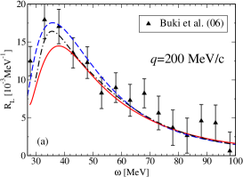
Figure 1: (Color online) Longitudinal response function for $q=200$ and $100$ ${\rm MeV}/c$ with the AV18 (dashed), AV18+UIX (solid) and MT (dashed-dotted) potentials. Data at $q\simeq 200$ ${\rm MeV}/c$ from Buki06 .

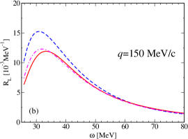
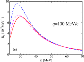
Figure 2: (Color online) Longitudinal response function for $q=200,150,100$ and $50$ ${\rm MeV}/c$ with the AV18 two-nucleon force only (dashed), and with the addition of the UIX (solid) or the TM’ (dashed-dotted) three-nucleon force.

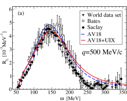
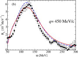
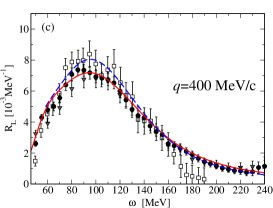
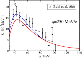
Figure 3: (Color online) $R_{L}(\omega,q)$ for $250\leq q\leq 500$ ${\rm MeV}/c$: calculations with AV18 (dashed) and AV18+UIX (solid). Data from Bates (squares), Saclay (circles), Carlson02 (triangles down), and Buki06 (triangles up).

In this section we present results on $R_{L}$, focusing on the evolution of dynamical effects as the momentum transfer decreases. In Fig. 1, we show $R_{L}$ at constant $q=200$ and 100 MeV/c. As already shown in PRL09 one has a large quenching effect due the 3NF, which is strongest at lower $q$. One should notice that such an effect is not simply correlated to the under-binding of the AV18 potential (binding energy $E_{B}$= 24.35 MeV in the present LIT calculation, with higher EIHH precision $E_{B}$= 24.27 MeV Gazit06 ). In fact, if this was the case, the results with the Malfliet-Tjon potential (MT) MaT69 , which gives a slight over-binding of ⁴He ($E_{B}$=30.56 MeV), would lay even below those obtained with AV18+UIX ($E_{B}$= 28.40). On the contrary the MT curve is situated between the curves with and without 3NF.

We would like to mention that we do not give results for the very threshold region, where one has a 0⁺ resonance Wal70 . In our present calculation we are not able to resolve this narrow resonance, therefore we subtract its contribution before inversion as we do for the elastic peak REPORT07 . This procedure of course does not affect the result above the resonance.

Given the large 3NF effect at lower $q$ it is interesting to see whether there is a dependence of the results on the 3NF model itself. To this end we have performed the calculation using also the Tucson Melbourne (TM’) TMprime three-nucleon force. While the UIX force contains a two-pion exchange and a short range phenomenological term, with two 3NF parameters fitted on the triton binding energy and on nuclear matter density (in conjunction with the AV18 two-nucleon potential), the TM’ force is not adjusted in this way. It includes two pion exchange terms where the coupling constants are taken from pion-nucleon scattering data consistently with chiral symmetry.

Our results with the TM’ force are obtained using the same model space as for the UIX potential and the accuracy of the convergence for the LIT is found to be at a percentage level, in analogy to that of the UIX as described in PRL09 . The cutoff of the TM’ force has been adjusted on triton binding energy, when used in conjunction with the AV18 NN force. With a cutoff $\Lambda=4.77m_{\pi}$, where $m_{\pi}$ is the pion mass, we obtain the following binding energies 8.47 MeV (³H) and 28.46 MeV (⁴He). We would like to emphasize that the ⁴He binding energy is practically the same as for the AV18+UIX case (as already found in Nogga02 ).

In addition to what is shown in our recent Letter PRL09 , here we investigate also other low-$q$ values. Figure 2 shows that the increase of 3NF effects with decreasing $q$ is confirmed. Moreover it becomes evident that also the difference between the results obtained with two 3NF models increases with decreasing $q$. One actually finds that the shift of the peak to higher energies in the case of UIX generates for $R_{L}$ a difference up to about 10% on the left hand sides of the peaks. This is a very interesting result. It represents the first case of an electromagnetic observable considerably dependent on the choice of the 3NF. In the light of these results it would be very interesting to repeat the calculation with EFT two-and three-body potentials EM ; EGM . At the same time it would be highly desirable to have precise measurements of $R_{L}$ at low $q$. This could serve either to fix the low-energy constants (LEC) of the effective field theory 3NF or to possibly discriminate between different nuclear force models.

In Fig. 3, an overview of the results obtained for larger $q$ is given, showing also the comparison with existing experimental data. One sees that the 3NF results are closer to the data, this is particularly evident at $q=300$ MeV/c. However, the 3NF effect is generally not as large as for the lower momentum transfers shown in Figs. 2 and 3. In some cases the quenching of the strength due to the 3NF is comparable to the size of the error bars, particularly for the data from Ref. Bates . The largest discrepancies with data are found at $q=500$ MeV/c. While the height of the peak is well reproduced by the result with 3NF, the width of the experimental peak seems to be somewhat narrower than the theoretical one. On the other hand one has to be aware that relativistic effects are not completely negligible at $q=500$ MeV/c. They probably play a similar role as found in the electro-disintegration of the three-nucleon systems (see e.g. Ref. RL3B ). In the case of $q=$ 250 MeV/c the experimental results are not sufficiently precise to draw a conclusion.

IV Multipole Analysis

Figure 4: Response functions of the lowest isovector (upper panel) and isoscalar (lower panel) Coulomb multipoles, starting with the monopole and consecutively adding higher multipoles up to $J_{max}=7$ for ${q}=500$ MeV/c (left) and $J_{max}=2$ for ${q}=100$ MeV/c (right) in case of the AV18+UIX potential.

It is interesting to analyze the results of $R_{L}$ in terms of its multipole contributions. Using Eq. (5) on the right-hand-side of Eq. (8), one can decompose ${\cal L}_{L}(\sigma,q)$ into a sum of multipole contributions ${\cal L}^{J,X}(\sigma,q)$. We have calculated each of them separately, solving the corresponding equations (8). After the inversion of the transform we have obtained the various multipole responses. By multiplying them with the isoscalar/isovector nucleon form factors we generate the multipole contributions to the longitudinal response function $R_{L}^{J,X}(\omega,q)$. In Fig. 4 we show how the isoscalar and isovector parts of $R_{L}$ are built up from their multipole contributions at a higher (500 MeV/c) and a lower (100 MeV/c) value of $q$. As expected, the higher the momentum transfer, the larger the number of multipoles that have to be considered to reach convergence. For $q=500$ MeV/c up to seven multipoles are considered, while for $q=100$ MeV/c only three multipoles are required for a converged result. Regarding the strength distribution among the multipoles two facts are evident: i) at higher $q$ the strength is almost equally distributed among the first isovector multipoles, while in the isoscalar channel the quadrupole gives the largest contribution; ii) at low $q$, as expected, the response is dominated by the isovector dipole contribution. While the isoscalar dipole is completely negligible, the isoscalar quadrupole contributes a few percent. A careful reader may notice that the isoscalar response at $q=100$ MeV/c does not seem to show a convergence in the multipole decomposition. As already mentioned, the isoscalar dipole is negligible (explaining why the curve labeled with “0” is overlapping with the “+1” one), and a similarly negligible strength is found for the multipoles higher than the quadrupole. This fact is also seen in Fig. 5, where the total strength of the various multipoles is shown for $q=100$, 300 and 500 MeV/c.

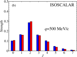
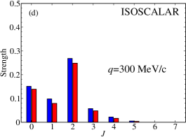
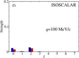
Figure 5: (Color online) Isovector (left) and isoscalar (right) multipole strength distribution of $R_{L}$ at $q$=500, 300 and 100 MeV/c in case of the AV18 and AV18+UIX potentials.

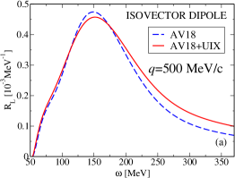
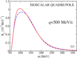
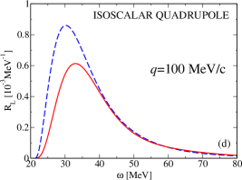
Figure 6: (Color online) Response functions of the isovector dipole and isoscalar quadrupole for ${q}=500$ and ${q}=100$ MeV/c with the AV18 (dashed) and AV18+UIX (solid) potentials.

At $q=$100 MeV/c the $J=1$ and 3 multipoles of the isoscalar response are tiny. The $J>3$ multipoles are neglected in Figs. 1, 2 and 4 for the $q\leq$100 MeV/c kinematics. We would like to point out that the total strengths presented in Fig. 5 do not contain the nucleon form factors. The strengths can be obtained by integrating in energy (up to infinity) the inversion of ${\cal L}^{J,X}(\sigma,q)$ (non-energy weighted sum rule) or just by taking the norm of the right-hand-side of Eq. (8) for each multipole, i.e. the norm of $\hat{C}^{J,X}(q)|{\Psi_{0}}\rangle$.

In Fig. 5, 3NF effects are illustrated in addition. The three shown $q$ values give an idea of the evolution of the effect from the short range to the long range regime. At the highest $q$ value the three strongest contributions are given by the isovector dipole and the isoscalar and isovector quadrupole. They are enhanced by the 3NF, while all other multipoles are decreased, resulting in a net small quenching effect. At $q$= 300 MeV/c one notices a kind of transition situation where only the still dominating isovector dipole strength is increased by the 3NF, while all other multipoles are quenched. At $q=100$ MeV/c the strength of all multipoles is decreased by the 3NF resulting in an overall sizable quenching effect.

In Fig. 6, the effect described above shows up more clearly in the energy distribution of the dominant multipole contributions (isovector dipole, isoscalar quadrupole) at $q=$ 500 and 100 MeV/c. In particular at $q=$ 500 MeV/c the increase of the strength due to the 3NF in the isovector dipole channel is found mainly in the high energy tail, while in the isoscalar quadrupole the increase is found around the peak. At $q=$ 100 MeV/c the situation is different in that the quenching of the strength due to the 3NF concentrates in the peak region, for both multipoles. The net result of this mechanism is the increase of the 3NF quenching effect with decreasing $q$ that was evident in Fig. 2.

Here we would like to comment on the fact that the large contribution of the 3NF at low $q$ seems at variance with the smaller contribution to the photoabsorption cross section Gazit06 , dominated as well by the isovector dipole. The reason is twofold. It has to do on the one hand with the correct use of the Siegert theorem, and on the other hand with the common procedure to let theoretical cross sections start from the experimental threshold, also when the binding energies do not reproduce the experimental values. The detailed explanation is in order here. Because of charge conservation the relation (Siegert theorem) between the charge dipole matrix element ($C^{1,V}$) considered here and the electric dipole matrix element (E1) considered in the photon case implies the factor $(E_{n}-E_{0})$ (see also ee'MT ). The binding energy $(-E_{0})$ of ⁴He, however, is about 15% lower for AV18 than it is for AV18+UIX. One has the following consequences. In the AV18+UIX case of Ref. Gazit06 the result of the squared matrix element is multiplied by $(E_{n}-E_{0})$ which is equal to $\omega_{\gamma}$, while in the AV18 case a multiplication by $(E_{n}-E_{0})$ implies a smaller multiplicative factor. Therefore the quenching three-body effect results to be smaller. It is only thereafter that the AV18 ⁴He total photoabsorption cross section is shifted to the experimental threshold.

One might question the procedure of shifting the theoretical cross sections to the experimental threshold, but without such a shift all 3NF effects would be much amplified in the photoabsorption cross section and even in the present response function results. However, in this case one could say that they are in a way “trivial binding effects”.

V Integral properties of $R_{L}$

There are many examples in different fields of physics where one is not able to access a certain observable, but only some of its integral properties. Sum rules ($n^{th}$ moments of the energy distribution) REP91 are well known examples. They contain a certain amount of often very useful information about the observable, but a limited one. The more sum rules one knows, the larger the amount of information at disposal. Integral transforms can also be viewed as a special form of sum rules. While sum rules map an energy dependent observable into a set of $n$ discrete values, integral transforms map the same observable into a set of continuous values.

Reconstructing the searched observable from its integral properties can be very difficult, since very often only a limited number of moments are known or in case of integral transforms the result of the mapping does not resemble at all the observable of interest. This is not the case for the LIT. An example is illustrated in Fig. 7a where we compare $R_{L}(\omega,q=300\,{\rm MeV/c})$ for the AV18+UIX potential (as in Fig. 3e) with the corresponding LIT, ${\cal L}_{L}(\sigma,q)$, calculated using a typical value of $\sigma_{I}$ (20 MeV). One notices the similarity between the shape of the response function and of its integral transform. This similarity is due to the fact that the Lorentz kernel is a representation of the $\delta$-function. It is this property that makes the inversion of the integral transform TIK77 reliable and sufficiently accurate for the Lorentz kernel. This situation has to be confronted with the Laplace transform. The Laplace transform of $R_{L}$, called Euclidean response, is given by Eucl94

$${\cal E}(\tau,q)=\int_{\omega_{th}}^{\infty}\,d\omega\,\exp\left[-\tau\left(\omega-\frac{q^{2}}{2m}\right)\right]\frac{R_{L}(\omega,q)}{Z|G_{E}^{p}(Q^{2})|^{2}}\,.$$ (14)

Fig. 7b shows how $\cal E(\tau)$ exhibits a completely different form than $R_{L}(\omega,q)$. It is interesting to observe that even in the $\tau$-space the Euclidean response obtained using only the two-body potential gives a result much different from that which includes the 3NF. However, what is not evident from ${\cal E}(\tau)$ is in which energy region the contribution of the 3NF is important.

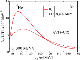
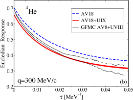
Figure 7: (Color online) Longitudinal response function $R_{L}$ (solid) at $q=300$ MeV/c with its Lorentz Integral Transform (dashed) for the AV18+UIX potential (a). The LIT has been multiplied by $\frac{\sigma_{I}}{\pi}$ to normalize the integral kernel with respect to Eq. (7). Euclidean longitudinal response for the same momentum transfer (b): comparison of the GFMC calculation Eucl94 for the AV8+UVIII potential (band between thin lines) and the result of this work with the AV18 (dashed) and AV18+UIX (solid).

Fig. 7b also shows a comparison of our results with those of Ref. Eucl94 obtained with the Monte Carlo method. The comparison is of interest, even if the potentials used in the two cases are slightly different (in Eucl94 the older versions of the Argonne and Urbana AV8 and UVIII had been used). At $\tau$ larger than 0.02, our result with AV18+UIX lies within the error band of the Monte Carlo numerical noise. At smaller $\tau$, and in particular at $\tau=0$ Fig. 7b shows a discrepancy between the present ${\cal E}(\tau,q)$ and that of Ref. Eucl94 . This is certainly due to the different potentials used. The ${\cal E}(0)$ value corresponds to the zero-th moment of $R_{L}(\omega,q)$. This is a classical integral property of $R_{L}(\omega,q)$ that has been much discussed in the literature under the name of Coulomb sum rule (CSR) (for a review see REP91 ; Ben08 ). The sum rule consists in connecting the integral of the inelastic longitudinal response to the number of protons and to the Fourier transform of the proton-proton correlation function $\rho_{pp}(s)$, i.e the probability to find two protons at a distance $s$. In fact for the charge density operator of Eq.( 3) (and neglecting the neutron charge form factor) one has

$${\rm CSR}(q)\equiv\!\int_{\omega_{el}^{+}}\!\!\!\!\!\!d\omega{\frac{R_{L}(\omega,q)}{|G_{E}^{p}(Q^{2})|^{2}}}\!=\!Z+Z(Z-1)f_{pp}(q)-Z^{2}|F(q)|^{2}\!,$$ (15)

where $\omega_{el}$ represents the elastic peak energy, $f_{pp}(q)$ is the Fourier transform of $\rho_{pp}(s)$ and $F(q)$ is the nuclear elastic form factor. (Another interesting sum rule concerning the second moment of $\rho_{pp}(s)$ has been considered in Ref. tetraedro , where one finds $\langle s^{2}\rangle=5.67$ fm² for AV18+UIX) The main interest in CSR($q$) has been considered its very simple model independent large $q$ limit, i.e. the number of protons. information about the proton-proton correlation function.

In Fig. 8, $f_{pp}(q)$ is shown in comparison with the results of Ref. Carlson02 obtained with the same potential, including in addition higher relativistic order corrections as well as exchange operators, neglected here. We can make the following observations: i) the perfect agreement of the two results when the operator in Eq. (3) is used shows the great accuracy of the two calculations; ii) the contributions of exchange currents, become negligible below $q=300$ MeV. This means that at low $q$ the physical interpretation of $f_{pp}(q)$ as Fourier transform of $\rho_{pp}(s)$ is safe. Therefore, in principle, the comparison theory-experiment would allow to study microscopically the largely unknown long range correlations. iii) as one can see in Fig. 8b the effect of the 3NF on $f_{pp}(q)$ is up to 15% in the “safe” region below $q$=300 MeV/c This gives an idea of the required experimental accuracy.

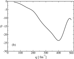
Figure 8: (Color online) (a): $f_{pp}(q)$ in the CSR (Eq. (15)) with AV18 (dashed) and AV18+UIX (solid) potentials. Dots: results from Carlson02 with the one-body density operator of Eq.( 3), triangles: results from Carlson02 with two-body density operator. (b): percent difference between the curves in (a)

Unfortunately, obtaining the “experimental“ CSR($q$) (as well as ${\cal E}(0)$) is a non trivial task, due to the necessity of extrapolating data up to infinite energies, even crossing the photon point, where $(e,e^{\prime})$ measurements do not have access. Different extrapolating functions have been proposed. They have been used also recently in Ref. Buki06 . Our results can help to determine these tail contributions. They can in fact be obtained subtracting from CSR($q$) the experimental sum of the data up to the last measured point at $\omega_{max}$. From the Saclay data Saclay at $q=$300 and 350 MeV/c we have estimated this high energy contribution to be about 7% of the CSR. The effect becomes twice as large for the higher $q$-values. However, while this procedure would be safe enough at low $q$, at large $q$ this estimate can be inaccurate because of the neglect of relativistic effects, two-body operators and the role of neutron form factor. In general it would be desirable that the tail contribution does not overcome the 3NF effect. Therefore accurate data should be taken as far in energy as possible. Of course they cannot overcome the photon point, therefore it is interesting to calculate the contribution of the tail beyond it. In Table 1, one sees that for $q$-values up to 200 MeV/c the contribution of the time-like region remains very low reaching at most 1.5%.

The previous discussion gives an idea of the experimental accuracy required to access the information about the proton-proton correlation function.

Table 1: Theoretical CSR for low $q$ with the AV18+UIX potential in comparison with $I^{th}_{\gamma}=\int_{\omega_{el}^{+}}^{\omega=q}d\omega R_{L}^{exp}(q,\omega)/|G_{E}^{p}(Q^{2})|^{2}$. The percentage contribution of the time-like response is also shown.

$q$ [MeV/c]	CSR$(q)$	$I^{th}_{\gamma}$	$\%$ time-like
50	3.88	3.86	0.5
100	3.57	3.55	0.6
150	3.17	3.14	0.9
200	2.79	2.74	1.5

VI Conclusions

In this paper we have analyzed 3NF effects on the electron scattering longitudinal response function at several kinematics. The most interesting results regard momentum transfers between 50 and 250 MeV/c. Large effects of 3NFs are found for two different three-body potentials (Urbana IX and Tucson-Melbourne^′). We also observe that the 3NF effects differ by non negligible amounts for the two three-body force models. Since the difference between the two results increases with decreasing momentum transfer one can ascribe it to rather different long range correlations generated by the the two forces. This fact results from the difference in the continuum excitation spectra of the two potentials. In light of this observation one can envisage the possibility to discriminate also between phenomenological and effective field theory potentials, if precise experimental data were available at these kinematics.

Three-body force effects have been analyzed separately in the various multipoles contributing to the response. Below $q=$ 300 MeV/c a cooperative quenching effect in all multipoles has been found.

Integral properties of the longitudinal response function have also been addressed. In particular the possibility to extract information about the long range behavior of the proton-proton correlation function has been discussed. In relation to this it has been underlined how the present results can be used in determining the energy tail contributions to the Coulomb sum rule.

In general it has been emphasized that different from the search for the short range correlations, the study of the long range ones is not affected by complications due to relativistic and two-body contributions. Therefore a Rosenbluth separation of inclusive electron scattering cross section of ⁴He at momentum transfer $q\leq 200$ MeV/c would be of high value in view of a more accurate determination of the three-body force and in general of the long range dynamics of this system.

Acknowledgments

We would like to thank Alexandr Buki for providing us with information about the data of Ref.Buki06 . This work was supported in part by the Natural Sciences and Engineering Research Council (NSERC) and by the National Research Council of Canada. The work of N. Barnea was supported by the Israel Science Foundation (grant no. 361/05). Numerical calculations were partially performed at CINECA (Bologna).

References

- (1) S. C. Pieper, K. Varga, and R. B. Wiringa, Phys. Rev. C 66, 044310 (2002) and references therein.
- (2) P. Navràtil, V. G. Gueorguiev, J. P. Vary, W. E. Ormand, and A. Nogga, Phys. Rev. Lett. 99, 042501 (2007) and referemces therein.
- (3) A. Kievsky, S. Rosati, M. Viviani, L. E. Marcucci, and L. Girlanda, J. Phys. G 35, 063101 (2008) and references therein.
- (4) A. Deltuva, A. C. Fonseca, and S. K. Bogner, Phys. Rev, C 77, 024002 (2008).
- (5) J. Carlson, J. Jourdan, R. Schiavilla, and I. Sick, Phys. Rev. C 65, 024002 (2002).
- (6) V. D. Efros, W. Leidemann, and G. Orlandini, Phys. Lett. B 338, 130 (1994).
- (7) V. D. Efros, W. Leidemann, G. Orlandini, and N. Barnea, J. Phys. G: Nucl. Part. Phys. 34, R459 (2007).
- (8) T.-S. Park et al., Phys. Rev. C 67, 055206 (2003).
- (9) S. Bacca, N. Barnea, W. Leidemann, G. Orlandini, Phys. Rev. Lett. 102, 162501 (2009).
- (10) J. M. Eisenberg and W. Greiner, Excitation mechanisms of the nucleus, North-Holland Publishing Company, Amsterdam, 1970.
- (11) N. Barnea, W. Leidemann, and G. Orlandini, Phys. Rev. C 61, 054001 (2000); Nucl. Phys. A 693, 565 (2001).
- (12) N. Barnea, V. D. Efros, W. Leidemann, and G. Orlandini, Few-Body Syst. 35, 155 (2004).
- (13) V. D. Efros, W. Leidemann, and G. Orlandini, Few-Body Syst.26, 251 (1999).
- (14) D. Andreasi, W. Leidemann, C. Reiß, and M. Schwamb, Eur. Phys. J. A 24, 361 (2005).
- (15) N. Barnea, V. D. Efros, W. Leidemann, and G. Orlandini, arXiv:0906.5421.
- (16) S. Galster et al., Nucl. Phys. B 32, 221 (1971).
- (17) A. Yu. Buki, I. S. Timchenko, N. G. Shevchenko, and I. A. Nenko, Phys. Lett. B 641, 156 (2006).
- (18) D. Gazit, S. Bacca, N. Barnea, W. Leidemann, and G. Orlandini, Phys. Rev. Lett. 96, 112301 (2006).
- (19) R. A. Malfliet and J. A. Tjon, Nucl. Phys. A127, 161 (1969).
- (20) Th. Walcher, Phys. Lett. B 31, 442 (1970); Z. Phys. 237, 368 (1970).
- (21) S. A. Coon and H. K. Hahn, Few-Body Syst. 30, 131 (2001).
- (22) A. Nogga, H. Kamada, W. Glöckle, B.R. Barrett, Phys. Rev. C 65, 054003 (2002).
- (23) D. R. Entem and R. Machleidt, Phys. Rev. C68, 041001(R) (2003).
- (24) E. Epelbaum, W. Glöckle and U. G. Meißner, Nucl. Phys. A747, 362 (2005).
- (25) S. A. Dytman et al., Phys. Rev. C 38, 800 (1988).
- (26) A. Zghiche et al., Nucl. Phys. A572, 513 (1994).
- (27) V. D. Efros, W. Leidemann, G. Orlandini, and E. L. Tomusiak, Phys. Rev. C 72, 011002 (2005).
- (28) S. Bacca, H. Arenhövel, N. Barnea, W. Leidemann, and G. Orlandini, Phys. Rev. C 76, 014003 (2007).
- (29) G. Orlandini and M. Traini, Rep. Prog. Phys. 54, (1991) 257.
- (30) A. N. Tikhonov and V. Y.Arsenin, Solutions of Ill–Posed Problems, V. H. Winston and Sons Pub.Co,Washington, DC, 1977.
- (31) J. Carlson and R. Schiavilla, Phys. Rev.C 49, 2880 (1994).
- (32) O. Benhar, D. Day, and I. Sick, Rev. Mod. Phys. 80, 189 (2008).
- (33) D. Gazit, N. Barnea, S. Bacca, W. Leidemann, and G. Orlandini, Phys. Rev.C 74, 061001 (2006).