Consensus in Correlated Random Topologies: Weights for Finite Time Horizon

Abstract

We consider the weight design problem for the consensus algorithm under a finite time horizon. We assume that the underlying network is random where the links fail at each iteration with certain probability and the link failures can be spatially correlated. We formulate a family of weight design criteria (objective functions) that minimize $n$, $n=1,...,N$ (out of $N$ possible) largest (slowest) eigenvalues of the matrix that describes the mean squared consensus error dynamics. We show that the objective functions are convex; hence, globally optimal weights (with respect to the design criteria) can be efficiently obtained. Numerical examples on large scale, sparse random networks with spatially correlated link failures show that: 1) weights obtained according to our criteria lead to significantly faster convergence than the choices available in the literature; 2) different design criteria that corresponds to different $n$, exhibits very interesting tradeoffs: faster transient performance leads to slower long time run performance and vice versa. Thus, $n$ is a valuable degree of freedom and can be appropriately selected for the given time horizon.

Index Terms—  consensus, weight design, convex optimization, time horizon, correlated link failures

1 Introduction

We consider the design of the weights for the consensus algorithm under a finite time horizon. We assume the network is random with links failing at each iteration with certain probability (see also [1, 2, 3]). The link failures are temporally uncorrelated but can be spatially correlated, which is a better suited assumption for wireless sensor networks (WSNs) than spatially uncorrelated failures. Reference [4] optimizes the weights for $static$ network topologies. The weight design in [4] leads to a convex problem of maximizing the algebraic connectivity of the (weighted) graph Laplacian with respect to the weights. In [5], we showed that the weight optimization for $random$ network topologies can be cast as a convex optimization problem. In this paper, we consider also the weight design for random topologies, but here consensus is over a finite number of iterations, i.e., under a $finite$ $time$ $horizon$. This problem is of interest in WSNs, where the number of iterations available can be limited to a small number due to the small power budget of sensors. Also, in certain applications, e.g., distributed detection of critical events (e.g., fire), result must be provided within certain critical time. Weight design with finite time horizon requires a new approach, different than [5], since it must account for the transient phase of the consensus algorithm. We first explain our methodology for solving the problem on static networks; we show that, under a finite time horizon of $k$ iterations, not only the slowest mode, but all the modes of the consensus error dynamics should be taken into account. This leads to the formulation of a family of convex objective functions, indexed by $n$, that minimize the sum of the $n$ largest eigenvaules that correspond to the $n$ slowest modes, $n=1,...,N$, of the error state matrix. We generalize all the results to random networks with spatially correlated links. We show that the objective functions are still convex for random topologies. Hence, globally optimal weights (with respect to the defined criteria) can be efficiently obtained by numerical optimization. The weight design [5] is a special case of the functions family proposed here when $n=1$. Numerical examples on sparse, large scale networks with spatially correlated link failures show that: 1) the weights from our design family lead to significantly faster convergence than the available choices in the literature; 2) different choices from our family (that correspond to different choice of $n$) exhibit very interesting tradeoffs: better transient performance leads to worse time asymptotic performance and vice versa. Thus, depending on the given time horizon, one can choose the appropriate cost function (i.e., $n$) to achieve the desired performance.

2 Problem model

We follow the model of a random network as in [6], except that we assume that the links can be spatially correlated, while in [6] they are uncorrelated. We briefly introduce relevant objects and notation. The supergraph $G=(V,E)$ is the graph that collects all the links with non zero probability of being alive. ($V$ is the set of nodes, and $E$ is the set of undirected links.) At any time step $k$: 1) link $\{i,j\}\in E$ is active with probability $P_{ij}$; 2) link $r$, incident to nodes $i$ and $j$, and link $s$, incident to nodes $l$ and $m$, are correlated with the corresponding cross variance $R_{rs}$. Consensus is an iterative distributed algorithm that computes the average $x_{\mbox{\scriptsize{avg}}}=\frac{1}{N}\sum_{i=1}^{N}x_{i}(0)$ of scalar sensor measurements (or some other data) $x_{i}(0)$ iteratively at each sensor $i$:

$$x_{i}(k+1)=\left(1-\sum_{j\in{O}_{i}}\mathcal{W}_{ij}(k)\right)x_{i}(k)+\sum_{j\in{O}_{i}}\mathcal{W}_{ij}(k)x_{j}(k)$$ (1)

In (1), $O_{i}$ denotes the neighborhood set of sensor $i$, i.e., ${O}_{i}=\{j:\,\,\{i,j\}\in E\}.$ Defining the state matrix $\mathcal{W}(k)=\left[\mathcal{W}_{ij}(k)\right]$ and the state vector $x(k)=(x_{1}(k),...,x_{N}(k))^{T}$ we have in compact form: $x(k+1)=\mathcal{W}(k)\,x(k).$ Also, it is straightforward to show (e.g., [4]) that the consensus error $e(k)=x(k)-x_{\mbox{\scriptsize{avg}}}\,1$ follows the dynamics:

$$e(k+1)=\left(\mathcal{W}(k)-J\right)e(k),\,\,J=\frac{1}{N}11^{T}.$$

We consider the case when $\mathcal{W}_{ij}(k)$, $\{i,j\}\in E$, is equal to a prescribed number $W_{ij}$ whenever link $\{i,j\}$ is alive and zero otherwise. Thus, $\mathcal{W}_{ij}(k)$ is a binary random variable for $\{i,j\}\in E$ ($\mathcal{W}_{ij}(k)=0$ if $\{i,j\}\notin E$). We design the weights $\{W_{ij}\}=\{W_{ij}\in\mathbb{R}:\,\,\{i,j\}\in E,\,\,i<j\}$ that lead to fast average consensus under a finite time horizon. We define a family of convex objective functions (criteria) that lead to fast consensus in random topologies. We first explain our methodology in the context of a static topology (section 3) and then consider correlated random topologies (section 4).

3 Static topology: Motivation example

We consider first that the network is static. Then, the state matrix $\mathcal{W}(k)=\mathcal{W}$ is deterministic and is given by: $\mathcal{W}_{ij}=W_{ij}$, $\{i,j\}\in E$; $\mathcal{W}_{ij}=0$, $\{i,j\}\notin E$; $\mathcal{W}_{ii}=1-\sum_{i\in O_{i}}W_{ij}$. We compute the eigenvalue decomposition of the matrix $\mathcal{W}-J$, $\mathcal{W}-J=Q\,\Lambda\,Q^{T},$ where the eigenvalues are ordered such that $|\lambda_{1}|\geq|\lambda_{2}|\geq...\geq|\lambda_{N}|=0$ ($\lambda_{N}=0$ since $\mathcal{W}1=1$ and $J1=1$.) A necessary and sufficient condition for the consensus algorithm (1) to converge is that $|\lambda_{1}|<1$ [4]. The consensus error can be written as:

$$\|e(k)\|^{2}=\sum_{i=1}^{N-1}\lambda_{i}^{2k}\,\left(q_{i}^{T}e(0)\right)^{2}=\sum_{i=1}^{N-1}\zeta_{i}^{2}(k)$$ (2)

Weight optimization for static topology has been studied in [4]. This reference proposes two different criteria (objective functions) to optimize the weights, the time asymptotic convergence rate $r_{\mathrm{as}}$ and the worst case per step convergence rate $r_{\mathrm{step}}$ defined as:

$$r_{\mathrm{as}} = \sup_{e(0)\neq 0}\lim_{k\rightarrow\infty}\left({\|e(k)\|}/{\|e(0)\|}\right)^{1/k}$$

$$r_{\mathrm{step}} = \sup_{e(k)\neq 0}{\|e(k+1)\|}/{\|e(k)\|}$$

Since the matrix $\mathcal{W}-J$ is symmetric, we have that $r_{\mathrm{as}}=r_{\mathrm{step}}=|\lambda_{1}|$, [4]. Thus, $r_{\mathrm{as}}$ and $r_{\mathrm{step}}$ both map to the minimization of $|\lambda_{1}|$ with respect to the weights $\{W_{ij}\}$. This is a convex optimization problem [4].

We argue that for small $k$ and for the optimal average performance, rather than the worst case performance, a criterion for minimization different than $|\lambda_{1}|$ should be considered. We give a motivational numerical example by considering a (static) connected network with $N=120$ nodes and $M=449$ edges. Figure 1 plots $\|e(k)\|^{2}$ averaged over 1000 different random initial conditions for two different weight choices: 1) the weights that minimize $|\lambda_{1}|$; 2) the Metropolis weights (MW), [1]. Metropolis weights are a heuristic weight choice and thus not optimal. However, in first 20 iterations, MW performs better. The reason is that minimization of $|\lambda_{1}|$ causes several other eigenvalues of $\mathcal{W}-J$ to be close in modulus to $\lambda_{1}$. Eqn. (2) clearly shows that, for a small number of iterations $k$, all nonzero eigenvalues $\lambda_{i}$ affect the error (since for small $k$ $\lambda_{i}^{2k}$ are not negligible, $i=1,...,N-1$ ). Thus, for small $k$, it is better to have many eigenvalues of $\mathcal{W}-J$ small in modulus than to minimize $|\lambda_{1}|$ at the cost of having large $\lambda_{2},\lambda_{3},...$.

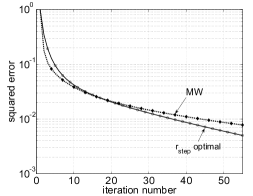
Fig. 1: Squared error versus iteration $k$ for static network.

In order to make all modes $\zeta_{i}(k)$ (eqn. (2)) small, we propose to minimize the sum of the squares of the eigenvalues $\lambda_{i}$, i.e., to minimize the function $\psi_{N}\left(\{W_{ij}\}\right):=\sum_{i=1}^{N-1}\lambda_{i}^{2}=\mathrm{tr}\left((W-J)^{2}\right)$. Further, we may reason as follows. For $k$ being very large, only the largest eigenvalue is of interest; for $k$ being very small, all the eigenvalues should be taken into account. For some medium range of the number of iterations, it is reasonable to try to minimize the $n$ largest eigenvalues of $\left(\mathcal{W}-J\right)^{2}$, $1<n<N$. This leads to the minimization of function $\psi_{n}\left(\{W_{ij}\}\right):=\sum_{i=1}^{n}\lambda_{i}^{2}$, i.e., to the following optimization problem:

$$\begin{array}[+]{ll}\mbox{minimize}&\psi_{n}\left(\{W_{ij}\}\right)\\ \mbox{subject to}&W_{ij}\in{\mathbb{R}},\,\,\{i,j\}\in{E}\\ &|\lambda_{1}|<1\end{array}$$ (3)

The constraint $|\lambda_{1}|<1$ assures that we search only over the weight choices for which the consensus algorithm converges. It can be shown (the proof is omitted here) that the functions $\psi_{n}(\cdot)$, $n=1,...,N-1$, are convex, and thus (3) is a convex problem.

Lemma 1

The function $\psi_{n}\left(\{W_{ij}\}\right)$ is convex for any $n=1,...,N-1$.

4 correlated random topology

We generalize the results from the previous section to the case of random network topology with spatially correlated link failures. Reference [5] studies the weight design for correlated random topology. Denote the consensus error covariance matrix by $\Sigma(k)=\mathrm{E}\left[e(k)e^{T}(k)\right]$. It can be shown that [5]:

$$\mathrm{tr}\left(\Sigma(k+1)\right)=\mathrm{tr}\left(\Sigma(k)\,\left(\mathrm{E}\left[\mathcal{W}^{2}\right]-J\right)\right)$$ (4)

Reference [5] minimizes $\phi_{1}\left(\{W_{ij}\}\right)=\lambda_{1}\left(\mathrm{E}\left[\mathcal{W}^{2}\right]-J\right)$. This quantity represents: 1) the worst case per step mean squared rate of convergence (eqn. (5)); 2) the upper bound on the time asymptotic convergence rate (eqn. (6)), see [7]:

$$\sup_{\mathrm{E}\left[e(k)e(k)^{T}\right]\succeq 0,\,\mathrm{E}\left[e(k)^{T}e(k)\right]\neq 0}\frac{\mathrm{E}\left[e(k+1)^{T}e(k+1)\right]}{\mathrm{E}\left[e(k)^{T}e(k)\right]}$$ (5)

$$\lim_{k\rightarrow\infty}\frac{1}{k}\mathrm{ln}\left(\frac{\|e(k)\|}{\|e(0)\|}\right)^{1/k}\leq 0.5\,\mathrm{ln}\left(\lambda_{1}\left(\mathrm{E}\left[\mathcal{W}^{2}\right]-J\right)\right)$$ (6)

Define the function

$$\phi_{n}\left(\{W_{ij}\}\right)=\sum_{i=1}^{n}\lambda_{i}\left(\mathrm{E}\left[\mathcal{W}^{2}\right]-J\right).$$ (7)

We remark that $\phi_{1}(\cdot)$ for random topology boils down to $\psi_{1}(\cdot)$ for static topology. Thus, minimization of $\phi_{1}$ boils down to minimization of $|\lambda_{1}(\mathcal{W}-J)|$ if the network is static. The same holds for the functions $\phi_{n}(\cdot)$ and $\psi_{n}(\cdot)$, $n=2,...,N-1$. This is because the matrix $\mathrm{E}\left[\mathcal{W}^{2}\right]-J$ is simply the matrix $\mathcal{W}^{2}-J=(\mathcal{W}-J)^{2}$ when the network is static. Thus, we propose to solve the following optimization problem:

$$\begin{array}[+]{ll}\mbox{minimize}&\phi_{n}\left(\{W_{ij}\}\right)\\ \mbox{subject to}&W_{ij}\in{\mathbb{R}},\,\,\{i,j\}\in{E}\\ &\phi_{1}\left(\{W_{ij}\}\right)<1\end{array}$$ (8)

Constraint $\phi_{1}\left(\{W_{ij}\}\right)<1$ restricts the search only over the points $\{W_{ij}\}$ for which the algorithm converges in mean squared sense. Special case $n=1$ is studied in [5]. We have the following result:

Lemma 2

The function $\phi_{n}\left(\{W_{ij}\}\right),\,n=1,...,N-1$, is convex.

The proof of Lemma 2 for $n=1$ is in [5], but we extend it to the case of arbitrary $n$, $n=2,...,N-1$. Due to lack of space it is omitted. In view of Lemma 2, optimization problem (8) is convex; hence, globally optimal $\{W_{ij}\}$ can be efficiently obtained.

5 Simulations

We consider a sparse geometric supergraph with $N=120$ nodes and $M=449$ edges. Nodes are uniformly distributed on a unit square and the pairs of nodes with distance smaller than a radius $r$ are connected by an edge. We define the formation probabilities by the following model: $P_{ij}=1-c_{1}\,\left(\delta_{ij}/r\right)^{2}$, $\{i,j\}\in E,\,\,c_{1}=0.6.$. Link $r$, incident to nodes $i$ and $j$, and link $s$, incident to nodes $l$ and $m$ (and $P_{ij}<P_{lm}$) are correlated at time $k$; the corresponding cross-variance is given by $R_{rs}=c_{2}\,P_{ij}\left(1-P_{rs}\right)$, $c_{2}=0.2$. The correlated binary random links are simulated by the method in [8]. We compare the performance of our solutions with the weight choices for random topologies previously proposed in the literature, namely with the Metropolis weights [1], and the weights proposed in [7], which we refer to as the supergraph based weights (SGBW). Figure 2 plots the mean squared error averaged over 100 different initial conditions. We compare the following weight choices: 1) MW; 2) SGBW; 3) weights obtained by minimizing $\phi_{1}$ (which also appear in [5]); 4) weights obtained by minimizing $\phi_{30}$. Numerical minimization of (8) is done by the subgradient algorithm for constrained minimization: if the current point $\{W_{ij}\}$ is feasible ($\phi_{1}\left(\{W_{ij}\}\right)<1$), we compute the subgradient step in the direction of the objective function $\phi_{n}$; 2) if the current point $\{W_{ij}\}$ is infeasible ($\phi_{1}\left(\{W_{ij}\}\right)\geq 1$), we compute the subgradient step in the direction of $\phi_{1}$ (constraint function).

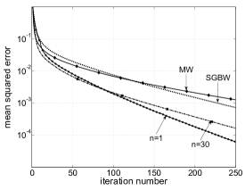
(a) Comparison of $\phi_{30}$ and $\phi_{1}$ with MW and SGBW

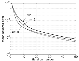
(b) Tradeoff in choice of $\phi_{1}$, $\phi_{15}$, $\phi_{30}$

Fig. 2: Random network: mean squared error versus iteration number averaged over 100 random initial conditions.

Figure 2 (a) shows that both $\phi_{1}$ and $\phi_{30}$ outperform SGBW and MW. To decrease the error to $1\%$, $\phi_{1}$ takes around 44 iterations; $\phi_{30}$ takes 37 iterations; SGBW and MW take more than 75 iterations to achieve $1\%$ precision. We see that $\phi_{1}$ and $\phi_{30}$ exhibit a tradeoff: in the transient regime (i.e., for small iterations $k$), $\phi_{30}$ performs better; for large $k$, $\phi_{1}$ performs better. For the precision of $1\%$, $\phi_{30}$ is a better choice (it saves 7 iterations compared to $\phi_{1}$, see also Figure 2(b)); for the precision of $0.1\%$, $\phi_{1}$ is a better choice (it saves around 15 iterations compared to $\phi_{30}$) (see Figure 2(a)). Figure 2(b) presents the performance for 3 different choices of $n$, $n=1,\,n=15,\,n=30$, in initial 50 iterations. We see that, for the $1\%$ precision, $\phi_{15}$ reduces by $25\%$ the number of iterations compared to $\phi_{1}$, from $43$ to $33$. Possibility of choosing different $n$ is valuable in practice. One can envision the application of the family $\{\phi_{n}\}$, for instance, in tracking applications, where combined technique of detection and estimation is used. In the first phase of tracking, target should be detected roughly in an area. This task can be done by distributed detection using consensus algorithm [9]. For this task, by nature of problem, high precision is not required, and thus one should choose $\phi_{30}$ criterion for fast solution. In the second phase of tracking, target trajectory is estimated, which can be done distributively based on consensus algorithm [1]. This task requires higher precision. For this phase, one could choose $\phi_{1}$ or $\phi_{15}$.

6 CONCLUSION

In this paper, we studied the weight design for a finite time horizon consensus with random topology and spatially correlated link failures. We addressed the problem of finding the optimal weights that yield the best average performance of the algorithm. We consider a finite time horizon, i.e., only a limited number of consensus iterations is available. We formulate a class of optimization problems for weight design under a finite time horizon. This class minimizes the sum of the $n$ largest eigenvalues of the matrix that describes the mean squared error dynamics , $n=1,...,N$. We show that the optimization problem is convex for arbitrary $n$ and hence can be efficiently globally solved. Numerical examples on large scale, sparse graphs with spatially correlated link failures show that, for any choice of $n$, optimization provides solutions better than the weight choices previously proposed in the literature. Also, the weight optimization for finite time consensus leads to very interesting tradeoffs: larger $n$ yields faster convergence in the transient regime and slower convergence in the long run regime. The parameter $n$ represents a valuable degree of freedom than can be appropriately set for given time horizon.

References

- [1] L. Xiao, S. Boyd, and S. Lall, “A scheme for robust distributed sensor fusion based on average consensus,” Los Angeles, California, 2005, pp. 63–70.
- [2] A. Tahbaz-Salehi and A. Jadbabaie, “Consensus over ergodic stationary graph processes,” to appear in IEEE Transactions on Automatic Control.
- [3] S. Kar and J. Moura, “Distributed consensus algorithms in sensor networks with imperfect communication: Link failures and channel noise,” IEEE Transactions on Signal Processing, vol. 57, no 1, pp. 355–369, Jan. 2009.
- [4] L. Xiao and S. Boyd, “Fast linear iterations for distributed averaging,” Syst. Contr. Lett., vol. 53, pp. 65–78, 2004.
- [5] D. Jakovetic, J. Xavier, and J. M. F. Moura, “Weight optimization for consensus algorithms with correlated switching topology,” submitted for publication, available at: http://arxiv.org/abs/0906.3736.
- [6] S. Kar and J. Moura, “Sensor networks with random links: Topology design for distributed consensus,” IEEE Transactions on Signal Processing, vol. 56, no.7, pp. 3315–3326, July 2008.
- [7] P. Denantes, F. Benezit., P. P Thiran, and M. Vetterli, “Which distributed averaging algorithm should I choose for my sensor network,” INFOCOM 2008, pp. 986–994.
- [8] B. Quadish, “A family of multivariate binary distributions for simulating correlated binary variables with specified marginal means and correlations,” Biometrika, vol. 90, no 2, pp. 455–463, 2003.
- [9] S. Kar, S. Aldosari, and J. Moura, “Topology for distributed inference on graphs,” IEEE Transactions on Signal Processing, vol. 56 No.6, pp. 2609–2613, June 2008.