Error analysis of tau-leap simulation methods

Abstract

We perform an error analysis for numerical approximation methods of continuous time Markov chain models commonly found in the chemistry and biochemistry literature. The motivation for the analysis is to be able to compare the accuracy of different approximation methods and, specifically, Euler tau-leaping and midpoint tau-leaping. We perform our analysis under a scaling in which the size of the time discretization is inversely proportional to some (bounded) power of the norm of the state of the system. We argue that this is a more appropriate scaling than that found in previous error analyses in which the size of the time discretization goes to zero independent of the rest of the model. Under the present scaling, we show that midpoint tau-leaping achieves a higher order of accuracy, in both a weak and a strong sense, than Euler tau-leaping; a result that is in contrast to previous analyses. We present examples that demonstrate our findings.

, and

t1Supported by NSF Grants DMS-05-53687 and DMS-10-09275. t2Supported by NSF Grant DMS-05-53687.

1 Introduction

This paper provides an error analysis for numerical approximation methods for continuous time Markov chain models that are becoming increasingly common in the chemistry and biochemistry literature. Our goals of the paper are two-fold. First, we want to demonstrate the importance of considering appropriate scalings in which to carry out error analyses for the methods of interest. Second, we wish to provide such an error analysis in order to compare the accuracy of two different approximation methods. We perform our analysis on the Euler tau-leaping method first presented in Gill2001 and a midpoint tau-leaping method developed below, which is only a slight variant of one presented in Gill2001 . The midpoint tau-leaping method will be demonstrated to be more accurate than Euler tau-leaping in both a strong and a weak sense, a result that is in contrast to previous error analyses. We will discuss why previous error analyses made differing predictions than does ours and argue that the scaling provided here, or variants thereof, is a more natural and appropriate choice for error analyses of such methods. We also provide examples that demonstrate our findings.

1.1 The basic model

The motivation for the class of mathematical models under consideration comes from chemistry and biochemistry, and more generally from population processes (though we choose the language of chemistry throughout the paper). We assume the existence of a chemical reaction system consisting of (i) $d$ chemical species $\{S_{1},S_{2},\ldots,S_{d}\}$ and (ii) a finite set of possible reactions, which we index by $k$. Each reaction requires some number of the species as inputs and provides some number of the species as outputs. For example, the reaction $S_{1}\to 2S_{2}$ would require one molecule of $S_{1}$ for the input and provide two molecules of $S_{2}$ for the output. If reaction $k$ occurs at time $t$, then the state of the system $X(t)\in\mathbb{Z}^{d}_{\geq 0}$ is updated via addition of the reaction vector $\nu_{k}\in\mathbb{Z}^{d}$, which represents the net change in the abundances of the underlying species:

$$X(t)=X(t-)+\nu_{k}.$$

Returning briefly to the example $S_{1}\to 2S_{2}$, the associated reaction vector for this reaction would be $[-1,2,0,\ldots,0]^{T}$. Finally, we denote by $\nu_{k}^{s}$ the vector in $\mathbb{Z}^{d}_{\geq 0}$ representing the source of the $k$th reaction. Returning again to the example $S_{1}\to 2S_{2}$, the source vector for this reaction is $\nu_{k}^{s}=[1,0,\ldots,0]^{T}$.

We assume that the waiting times for the $k$ reactions are exponentially distributed with intensity functions $\lambda_{k}\dvtx\mathbb{R}^{d}_{\geq 0}\to\mathbb{R}_{\geq 0}$. We extend each $\lambda_{k}$ to all of $\mathbb{R}^{d}$ by setting it to zero outside $\mathbb{R}^{d}_{\geq 0}$. This model is a continuous time Markov chain in $\mathbb{Z}^{d}_{\geq 0}$ with generator

$$(\mathcal{A}f)(x)=\sum_{k}\lambda_{k}(x)\bigl{(}f(x+\nu_{k})-f(x)\bigr{)},$$ (1)

where $f\dvtx\mathbb{Z}^{d}\to\mathbb{R}$ is arbitrary. Kolmogorov’s forward equation for this model, termed the “chemical master equation” in the chemistry and biology literature, is

$$\frac{d}{dt}P(x,t|\pi)=\sum_{k}P(x-\nu_{k},t|\pi)\lambda_{k}(x-\nu_{k})-\sum_{k}P(x,t|\pi)\lambda_{k}(x),$$

where for $x\in\mathbb{Z}^{d}_{\geq 0}$ $P(x,t|\pi)$ represents the probability that $X(t)=x$, conditioned upon the initial distribution $\pi$. One representation for path-wise solutions to this model uses a random time change of Poisson processes,

$$X(t)=X(0)+\sum_{k}Y_{k}\biggl{(}\int_{0}^{t}\lambda_{k}(X(s))\,ds\biggr{)}\nu_{k},$$ (2)

where the $Y_{k}$ are independent, unit-rate Poisson processes (see, e.g., KurtzPop81 ). Note that $\tilde{X}(t)\stackrel{{\scriptstyle\mathrm{def}}}{{=}}X(t)-\sum_{k}\int_{0}^{t}\lambda_{k}(X(s))\,ds\,\nu_{k}$ is a martingale with quadratic covariation matrix $[X]_{t}=\sum_{k}Y_{k}(\int_{0}^{t}\lambda_{k}(X(s))\,ds)\nu_{k}\nu_{k}^{T}$.

A common choice of intensity function for chemical reaction systems, and the one we adopt throughout, is mass action kinetics. Under mass action kinetics, the intensity function for the $k$th reaction is

$$\lambda_{k}(x) = \tilde{c}_{k}\pmatrix{x\cr x-\nu_{k}^{s}}=\frac{\tilde{c}_{k}}{\prod_{\ell=1}^{d}\nu_{k\ell}^{s}!}\prod_{\ell=1}^{d}\frac{x_{\ell}!}{(x_{\ell}-\nu^{s}_{k\ell})!}1_{\{x_{\ell}\geq 0\}}$$

$$\stackrel{{\scriptstyle\mathrm{def}}}{{=}} c_{k}\prod_{\ell=1}^{d}\frac{x_{\ell}!}{(x_{\ell}-\nu^{s}_{k\ell})!}1_{\{x_{\ell}\geq 0\}},$$

where $\tilde{c}_{k}$ is a positive constant and $c_{k}$ is defined by the above equation. Mass action kinetics arises by thinking of $\tilde{c}_{k}\Delta t$ as the approximate probability that a particular set of the molecules needed in the $k$th reaction will react over a time-period of size $\Delta t$, and then counting the number of ways such a reaction could happen. Implicit in the assumption of mass action kinetics is that the vessel under consideration is “well stirred.” For ease of notation, we will henceforth drop the indicator functions from our representation of mass action kinetics. More general rates will be discussed in the remark at the top of page six.

1.2 Numerical methods

There are a number of numerical methods that produce statistically exact sample paths for the model described above. These include the stochastic simulation algorithm, better known as Gillespie’s algorithm Gill76 , Gill77 , the first reaction method Gill76 and the next reaction method Anderson2007a , gibson2000 . All such algorithms perform the same two basic steps multiple times until a sample path is produced over a desired time interval: first, conditioned on the current state of the system the amount of time that passes until the next reaction takes place, $\Delta$, is computed and second the specific reaction that has taken place is found. If, however, $\sum_{k}\lambda_{k}(X(t))\gg 0$ then $\Delta\approx(\sum_{k}\lambda_{k}(X(t)))^{-1}\ll 1$ and the time needed to produce a single exact sample path over a time interval can be prohibitive.

The approximate algorithm “tau-leaping” was developed by Dan Gillespie in Gill2001 in an effort to overcome the problem that $\Delta$ may be prohibitively small. The basic idea of tau-leaping is to hold the intensity functions fixed over the time interval $[t_{n},t_{n}+h]$ at the values $\lambda_{k}(X(t_{n}))$, where $X(t_{n})$ is the current state of the system, and, under this assumption, compute the number of times each reaction takes place over this period. As the waiting times for the reactions are exponentially distributed, this leads to the following algorithm.

Algorithm 1 ((Euler tau-leaping)).

Set $Z(0)=X(0)$, $t_{0}=0$, $n=0$ and repeat the following until $t_{n+1}>T$. [(1)]

Set $Z(t_{n+1})=Z(t_{n})+\sum_{k}\mathcal{P}_{k,n}(\lambda_{k}(Z(t_{n}))h)\nu_{k}$, set $t_{n+1}=t_{n}+h$ and set $n=n+1$, where $\mathcal{P}_{k,n}(x)$ are independent Poisson random variables with parameters $x$.

Several improvements and modifications have been made to the basic algorithm described above over the years. However, they are mainly concerned with how to choose the step-size adaptively Cao2006 , Gill2003 and/or how to ensure that population values do not go negative during the course of a simulation Anderson2007b , Cao2005 , Chatterjee2005 , and are not explicitly relevant to the current discussion.

Similar to (2), a path-wise representation of Euler tau-leaping can be given through a random time change of Poisson processes,

$$Z(t)=X(0)+\sum_{k}Y_{k}\biggl{(}\int_{0}^{t}\lambda_{k}\bigl{(}Z\circ\eta(s)\bigr{)}\,ds\biggr{)}\nu_{k},$$ (4)

where $\eta(s)=t_{n}$ if $t_{n}\leq s<t_{n+1}$ and the $Y_{k}$ are as before. Noting that $\int_{0}^{t_{n+1}}\lambda_{k}(Z\circ\eta(s))\,ds=\sum_{i=0}^{n}\lambda_{k}(Z(t_{i}))(t_{i+1}-t_{i})$ explains our choice to call this method “Euler tau-leaping.” Defining the operator

$$(\mathcal{B}_{z}f)(x)=\sum_{k}\lambda_{k}(z)\bigl{(}f(x+\nu_{k})-f(x)\bigr{)},$$ (5)

we see that for $t>0$

$$\mathbb{E}f(Z(t))=\mathbb{E}f\bigl{(}Z\circ\eta(t)\bigr{)}+\mathbb{E}\int_{\eta(t)}^{t}\bigl{(}\mathcal{B}_{Z\circ\eta(t)}f\bigr{)}(Z(s))\,ds,$$ (6)

so long as the expectations exist. Further, we note that $\tilde{Z}(t)\stackrel{{\scriptstyle\mathrm{def}}}{{=}}Z(t)-\sum_{k}\int_{0}^{t}\lambda_{k}(Z\circ\eta(s))\,ds\nu_{k}$ is a martingale with quadratic covariation matrix

$$[\tilde{Z}]_{t}=\sum_{k}Y_{k}\biggl{(}\int_{0}^{t}\lambda_{k}\bigl{(}Z\circ\eta(s)\bigr{)}\,ds\biggr{)}\nu_{k}\nu_{k}^{T}.$$

It is natural to believe that a midpoint type method would be more accurate than an Euler type method in many situations. We therefore define the function

$$\rho(z)\stackrel{{\scriptstyle\mathrm{def}}}{{=}}z+\frac{1}{2}h\sum_{k}\lambda_{k}(z)\nu_{k},$$

which computes an approximate midpoint for the system assuming the state of the system is $z$ and the time-step is $h$.

Algorithm 2 ((Midpoint tau-leaping)).

Set $\mathcal{Z}(0)=X(0)$, $t_{0}=0$, $n=0$ and repeat the following until $t_{n+1}>T$. [(1)]

Set $\mathcal{Z}(t_{n+1})=\mathcal{Z}(t_{n})+\sum_{k}\mathcal{P}_{k,n}(\lambda_{k}\circ\rho\circ\mathcal{Z}(t_{n})h)\nu_{k}$, set $t_{n+1}=t_{n}+h$ and set $n=n+1$, where $\mathcal{P}_{k,n}(x)$ are independent Poisson random variables with parameters $x$.

Similar to (2) and (4), $\mathcal{Z}(t)$ can be represented via a random time change of Poisson processes:

$$\mathcal{Z}(t)=X(0)+\sum_{k}Y_{k}\biggl{(}\int_{0}^{t}\lambda_{k}\circ\rho\circ\mathcal{Z}\circ\eta(s)\,ds\biggr{)}\nu_{k},$$

where $\eta(\cdot)$ is as before. For $\mathcal{B}_{z}$ defined via (5) and any $0<t$ and any function $f$

$$\mathbb{E}f(\mathcal{Z}(t))=\mathbb{E}f\bigl{(}\mathcal{Z}\circ\eta(t)\bigr{)}+\mathbb{E}\int_{\eta(t)}^{t}\bigl{(}\mathcal{B}_{\rho\circ\mathcal{Z}\circ\eta(t)}f\bigr{)}(\mathcal{Z}(s))\,ds.$$ (7)

Finally, $\tilde{\mathcal{Z}}(t)\stackrel{{\scriptstyle\mathrm{def}}}{{=}}\mathcal{Z}(t)-\sum_{k}\int_{0}^{t}\lambda_{k}\circ\rho\circ\mathcal{Z}\circ\eta(s)\,ds\,\nu_{k}$ is a martingale with quadratic covariation matrix $[\tilde{\mathcal{Z}}]_{t}=\sum_{k}Y_{k}(\int_{0}^{t}\lambda_{k}\circ\rho\circ\mathcal{Z}\circ\eta(s)\,ds)\nu_{k}\nu_{k}^{T}$. The main goal of this paper is to show that the midpoint tau-leaping algorithm is indeed more accurate than the Euler tau-leaping method under an appropriate, and natural, scaling described in Section 2.

Historically, the time discretization parameter for tau-leaping has been $\tau$, thus giving the method its name. We choose to break from this tradition and denote our time-step by $h$ so as not to confuse $\tau$ with a stopping time.

1.3 Previous error analyses

Under the scaling $h\to 0$, Rathinam et al. Rathinam2005 performed a consistency check of Euler tau-leaping and found that the local truncation error was $\mathcal{O}(h^{2})$ for all moments. They also showed that under this same scaling Euler tau-leaping is first order accurate in a weak sense in the special case that the intensity functions $\lambda_{k}$ are linear Rathinam2005 . Li extended these results by showing that as $h\to 0$ Euler tau-leaping has a strong error (in the $L^{2}$ norm) of order $1/2$ and a weak error of order one Li2007 , which agree with classical results pertaining to numerical analysis of SDEs driven by Brownian motions (see, e.g., KloedenPlaten92 ).

Under the scaling $h\to 0$, it is readily seen that midpoint tau-leaping is no more accurate than Euler tau-leaping. This follows since midpoint tau-leaping consists of making an $\mathcal{O}(h^{2})$ correction to the intensity functions used in Euler tau-leaping. As $h\to 0$, this correction becomes negligible as Poisson processes “ignore” $\mathcal{O}(h^{2})$ corrections, and the accuracy of the two methods will be the same.

We simply note that while the analyses performed in Rathinam2005 and Li2007 and the argument made in the previous paragraph are technically correct, performing an analysis as $h\to 0$, independent of the rest of the model, is at odds with the useful regime of tau-leaping. That is, tau-leaping would only be used in a regime where $h\gg\Delta$, where $\Delta$ is the expected amount of time between reactions, for otherwise an exact method would be performed. Therefore, we should require that

$$h\gg\biggl{(}\sum_{k}\lambda_{k}(Z(t))\biggr{)}^{-1}\quad\mbox{or}\quad h\sum_{k}\lambda_{k}(Z(t))\gg 1,$$ (8)

where $Z(t)$ is the state of the system. In Section 2, we will present a natural scaling for the models under consideration that does satisfy (8) and under which we will perform our analysis.

1.4 Paper outline

The remainder of the paper is organized as follows. In Section 2, we give some natural assumptions on the models considered in this paper and introduce the scaling under which we perform our analysis. In Section 3, we perform a strong error analysis for both the Euler and midpoint tau-leaping methods and show that midpoint tau-leaping is the more accurate of the two under our scaling. In Section 4, we perform a weak error analysis of the different methods and again conclude that the midpoint method is more accurate. In Section 5, we present numerical examples demonstrating our results.

2 Assumptions on the model

2.1 Scalings of the model and the algorithms

As discussed in the Intro- duction, tau-leaping methods will only be of use if the time-discretization parameter $h$ satisfies $h\sum_{k}\lambda_{k}(Z(t))\gg 1$ while $(\sum_{k}\lambda_{k}(Z(t)))^{-1}\ll 1$, where $Z(t)$ is the state of the system at time $t$. There are a number of ways for the second condition to hold and a modeling choice must be made. We make the following natural assumptions:

The initial abundance of each species scales with $V$ for some $V\gg 1$.

Each rate constant satisfies $c_{k}^{V}=\mathcal{O}(V^{1-\nu_{k}^{s}\cdot\vec{1}})$, where $\vec{1}=[1,1,\ldots,1]^{T}$. In particular, $c_{k}^{V}=d_{k}/V^{1-\nu_{k}^{s}\cdot\vec{1}}$ for some $d_{k}>0$. We will denote by $X^{V}$ the normalized process defined as the vector of abundances divided by $V$, and will denote by $\lambda_{k}^{V}$ the intensity function defined to be mass action kinetics with rate constants $c_{k}^{V}$. This scaling is the so called “classical scaling” and arises naturally by thinking of $V$ as the volume of the vessel in which the reactions are taking place multiplied by Avogadro’s number Kurtz72 . In this case, $X^{V}$ gives the concentration of each species in moles per unit volume. To understand the scaling for the rate constants, consider the case of a reaction requiring as input two constituent molecules: $S_{1}$ and $S_{2}$. Perhaps $S_{1}+S_{2}\to S_{3}$. It is reasonable to assume that the probability that a particular pair of $S_{1}$ and $S_{2}$ molecules meet, and react, in a small time interval is inversely proportional to the volume of the vessel. This same type of logic holds for the cases in which more than two molecules are needed for a reaction to take place (i.e., the probability that three particular molecules meet and react is inversely proportional to the volume squared). For the case that only one molecule is needed for a reaction to take place, it is reasonable to assume that the probability of such a reaction taking place in the next small interval of time for a particular molecule should not scale with the volume. See also Wilkinson2006 , Chapter 6.

Models that satisfy assumptions (i) and (ii) above have an important property that we will detail here and make use of later. Let $x(t)$ denote the solution to the deterministic initial value problem

$$\dot{x}(t)=F(x(t))\stackrel{{\scriptstyle\mathrm{def}}}{{=}}\sum_{k}d_{k}x(t)^{\nu_{k}^{s}}\nu_{k},\qquad x(0)=x_{0}\in\mathbb{R}^{d}_{\geq 0},$$ (9)

where $d_{k}$ is defined in assumption (ii) above, and where for any two vectors $u^{v}\stackrel{{\scriptstyle\mathrm{def}}}{{=}}u_{1}^{v_{1}}\cdots u_{d}^{v_{d}}$ and we adopt the convention that $0^{0}=1$. That is, $x(t)$ is the solution to the corresponding deterministically modeled chemical reaction system with mass action kinetics. It was shown in Kurtz72 , Kurtz78 that for any $\varepsilon>0$ and any $T>0$, if $X^{V}(0)=x(0)=x_{0}$, then

$$\lim_{V\to\infty}P\Bigl{\{}\sup_{t\in[0,T]}|X^{V}(t)-x(t)|\geq\varepsilon\Bigr{\}}\to 0.$$ (10)

Denoting $\lambda_{k}$ as deterministic mass action kinetics with rate constant $d_{k}$, it is an exercise to check that for any reaction, that is, zeroth order, first order, second order, etc., and any $x\in\mathbb{R}^{d}_{\geq 0}$

$$\lambda_{k}^{V}(Vx)=V\lambda_{k}(x)+\zeta_{k}^{V}(x),$$

where $\zeta_{k}^{V}$ is uniformly bounded in $V$ and is nonzero only if the reaction requires more than one molecule of a particular species as an input. For example, for the second order reaction $S_{1}+S_{2}\to S_{3}$ we have

$$\lambda_{k}^{V}(Vx)=\frac{d_{k}}{V}(Vx_{1})(Vx_{2})=Vd_{k}x_{1}x_{2}=V\lambda_{k}(x),$$

whereas for the second order reaction $2S_{1}\to S_{3}$ we have

$$\lambda_{k}^{V}(Vx)=\frac{d_{k}}{V}Vx_{1}(Vx_{1}-1)=Vd_{k}x_{1}^{2}-d_{k}x_{1}=V\lambda_{k}(x)+\zeta_{k}^{V}(x)$$

with $\zeta_{k}^{V}(x)=-d_{k}x_{1}$. The term $\zeta_{k}^{V}$ will have a true $V$ dependence if three or more molecules of a particular species are required as input. We now state the definition $A_{k}^{V}(x)\stackrel{{\scriptstyle\mathrm{def}}}{{=}}\frac{1}{V}\lambda_{k}^{V}(Vx)$, and note that for all $x\in\mathbb{R}^{d}_{\geq 0}$

$$A_{k}^{V}(x)=\lambda_{k}(x)+\frac{1}{V}\zeta_{k}^{V}(x)$$ (11)

and $A_{k}^{V}(x)\equiv 0$ if $x\notin\mathbb{R}^{d}_{\geq 0}$. Manipulating the definition of $A_{k}^{V}$ shows that for all $x\in\mathbb{R}^{d}$

$$\lambda_{k}^{V}(Vx)=VA^{V}_{k}(x).$$ (12)

The assumption of mass action kinetics is not critical to the analysis carried out in this paper. Instead, what is critical to this particular analysis is that our kinetics satisfies the scaling (12) for $A_{k}^{V}$ satisfying (11) with $\lambda_{k}$ sufficiently smooth.

We now choose a discretization parameter for the approximate methods that is dependent upon the assumptions of the model set out above. We let

$$h^{V}\stackrel{{\scriptstyle\mathrm{def}}}{{=}}1/V^{\beta},$$ (13)

where $0<\beta<1$. We note that this scaling satisfies the necessary requirements detailed above as

$$\biggl{(}\sum_{k}\lambda_{k}^{V}(Vx)\biggr{)}^{-1} = \mathcal{O}(V^{-1})\ll 1,$$

$$V^{-\beta}\biggl{(}\sum_{k}\lambda_{k}^{V}(Vx)\biggr{)} = \mathcal{O}(V^{1-\beta})\gg 1.$$

With this choice of time-step, we let $Z^{V}$ and $\mathcal{Z}^{V}$ denote the processes generated by Euler and midpoint tau-leaping, respectively, normalized by $V$. We can now state more clearly what the analysis of this paper will entail. We will consider the case of $V\gg 0$ by letting $V\to\infty$ and consider the relationship of the normalized approximate processes $Z^{V}$ and $\mathcal{Z}^{V}$ to the original process $X^{V}$, normalized similarly. Note that all three processes converge to the solution of (9). We will perform both weak and strong error analyses. In the strong error analysis, we will consider $L^{1}$ convergence as opposed to the more standard (at least for systems driven by Brownian motions) $L^{2}$ convergence. The reason for this is simple: the Itô isometry makes working with the $L^{2}$-norm easier in the Brownian motion case, whereas Poisson processes lend themselves naturally to analysis in the $L^{1}$-norm.

We remark that it is clear that the choice of scaling laid out in this section and assumed throughout the paper will not explicitly cover all cases of interest. For example, one may choose to use approximation methods when (i) the abundances of only a strict subset of the constituent species are in an $\mathcal{O}(V)$ scaling regime, or (ii) it is the rate constants themselves that are $\mathcal{O}(V)$ while the abundances are $\mathcal{O}(1)$, or (iii) there is a mixture of the previous two cases with potentially more than two natural scales in the system. Our analysis will not be directly applicable to such cases. However, the purpose of this analysis is not to handle every conceivable case. Instead, our purpose is to try and give a more accurate picture of how different tau-leaping methods approximate the exact solution, both strongly and weakly, in at least one plausible setting and we believe that the analysis detailed in this paper achieves this aim. Further, we believe that error analyses conducted under different modeling assumptions can be carried out in similar fashion.

2.2 Redefining the kinetics

Before proceeding to the analysis, we allow ourselves one change to the model detailed in the previous section. As we will be considering approximation methods in which changes to the state of the system are determined by Poisson random variables (which can produce arbitrarily large values), there will always be a positive probability that solutions will leave a region in which the scaling detailed above is valid. Multiple options are available to handle such a situation. One option would be to define a stopping time for when the process leaves a predetermined region in which the scaling regime is valid and then only perform the analysis up to that stopping time. Another option, and the one we choose, is to simply modify the kinetics by multiplying by a cutoff function that makes the intensity functions zero outside such a region. This has the added benefit of guaranteeing the existence of all moments of the processes involved. Note that without this truncation or some other additional assumption guaranteeing the existence of the necessary moments, some of the moment estimates that follow may fail; however, the convergence in probability and convergence in distribution results in Theorems 3.10 and 3.17 would still be valid.

Let $\gamma\geq 0$ be $C^{\infty}$ with compact support $\Omega_{\gamma}\subset\mathbb{R}^{d}_{>0}$, with $\gamma(x)=1$ for all $x\in B_{r}(x(t))$ for some $r>0$, where $x(t)$ satisfies (9). Now, we redefine our intensity functions by setting

$$\lambda_{k}^{V}(x)=\gamma(x/V)c_{k}^{V}\prod_{\ell=1}^{d}\frac{x_{\ell}!}{(x_{\ell}-\nu_{k\ell}^{s})!}\qquad\mbox{for }x\in\mathbb{R}^{d},$$ (14)

where $c_{k}^{V}$ still satisfies the scaling detailed in the previous section. It is easy to check that the redefined kinetics still satisfies $\lambda_{k}^{V}(Vx)=VA_{k}^{V}(x)$, where now $A_{k}^{V}(x)$ has also been redefined by multiplication by $\gamma(x)$. Further, the redefined $\lambda_{k}^{V}$ is identical to the previous function on the domain of interest to us. That is, they only differ if the process leaves the scaling regime of interest. For the remainder of the paper, we assume our intensity functions are given by (14). Finally, we note that for each $k$ we have the existence of an $L_{k}>0$ such that

$$\sup_{x\in\mathbb{R}^{d},|\alpha|<\infty}|D^{\alpha}A_{k}^{V}(x)|\leq L_{k}.$$ (15)

3 Strong error analysis for Euler and midpoint tau-leaping

Throughout this section, we assume a time discretization $0=t_{0}<t_{1}<\cdots<t_{N}=T$ with $t_{n}-t_{n-1}=h^{V}=V^{-\beta}$ for some $0<\beta<1$. In Section 3.1 we give some necessary technical results. In Section 3.2 we give bounds for $\sup_{t\leq T}\mathbb{E}|X^{V}(t)-Z^{V}(t)|$ and $\sup_{t\leq T}\mathbb{E}|X^{V}(t)-\mathcal{Z}^{V}(t)|$ in terms of $V$, where $X^{V}(t),Z^{V}(t)$ and $\mathcal{Z}^{V}(t)$ are the normalized processes and satisfy the representations

$$X^{V}(t) = X^{V}(0)+\frac{1}{V}\sum_{k}Y_{k}\biggl{(}V\int_{0}^{t}A_{k}^{V}(X^{V}(s))\,ds\biggr{)}\nu_{k},$$ (16)

$$Z^{V}(t) = X^{V}(0)+\frac{1}{V}\sum_{k}Y_{k}\biggl{(}V\int_{0}^{t}A_{k}^{V}\bigl{(}Z^{V}\circ\eta(s)\bigr{)}\,ds\biggr{)}\nu_{k},$$ (17)

$$\mathcal{Z}^{V}(t) = X^{V}(0)+\frac{1}{V}\sum_{k}Y_{k}\biggl{(}V\int_{0}^{t}A_{k}^{V}\circ\rho^{V}\circ\mathcal{Z}^{V}\circ\eta(s)\,ds\biggr{)}\nu_{k},$$ (18)

where

$$\rho^{V}(z)\stackrel{{\scriptstyle\mathrm{def}}}{{=}}z+\frac{1}{2}V^{-\beta}\sum_{k}A_{k}^{V}(z)\nu_{k}$$

and $\eta(s)=t_{n}$ for $s\in[t_{n},t_{n+1})$. In Sections 3.3 and 3.4, we use different couplings of the processes than those above to provide the exact asymptotics of the error processes $X^{V}-Z^{V}$ and $X^{V}-\mathcal{Z}^{V}$.

3.1 Preliminaries

We present some technical, preliminary concepts that will be used ubiquitously throughout the section. For a more thorough reference of the material presented here, see Kurtz86 , Chapter 6. We begin by defining the following filtrations that are generated by the Poisson processes $Y_{k}$:

$$\mathcal{F}_{\tilde{u}} \stackrel{{\scriptstyle\mathrm{def}}}{{=}} \sigma\{Y_{k}(s_{k})\dvtx s_{k}\leq u_{k}\},$$

$$\mathcal{F}_{u}^{i} \stackrel{{\scriptstyle\mathrm{def}}}{{=}} \sigma\{Y_{k}(r),Y_{i}(s)\dvtx k\neq i,s\leq u,r\in[0,\infty)\},$$

where $\tilde{u}$ is a multi-index and $u$ is a scalar.

Lemma 3.1

Suppose that $X(t)$ satisfies (2) with nonnegative intensity functions $\lambda_{k}$. For $t\geq 0$ and a choice of $k$,

$$\tau_{k}(t)=\int_{0}^{t}\lambda_{k}(X(s))\,ds$$ (19)

is an $\{\mathcal{F}_{u}^{k}\}$-stopping time.

For $u\geq 0$, let $\alpha(u)$ satisfy

$$\int_{0}^{\alpha(u)}\lambda_{k}(X(s))\,ds=u,$$

where we take $\alpha(u)=\infty$ if $\int_{0}^{\infty}\lambda_{k}(X(s))\,ds<u$. Then $\alpha(u)$ is adapted to $\mathcal{F}_{u}^{k}$ and $\{\tau_{k}(t)\leq u\}=\{t\leq\alpha(u)\}\in\mathcal{F}_{u}^{k}$.

Therefore, if the processes $X(t)$ and $Z(t)$ satisfy (2) with nonnegative intensity functions $\lambda_{k,1}$ and $\lambda_{k,2}$, respectively, then for $t,s\geq 0$ and a choice of $k$,

$$\mathbb{E}\biggl{|}Y_{k}\biggl{(}\int_{0}^{t}\lambda_{k,1}(X(r))\,dr\biggr{)}-Y_{k}\biggl{(}\int_{0}^{s}\lambda_{k,2}(Z(r))\,dr\biggr{)}\biggr{|}$$

(20)

$$\qquad=\mathbb{E}\biggl{|}\int_{0}^{t}\lambda_{k,1}(X(r))\,dr-\int_{0}^{s}\lambda_{k,2}(Z(r))\,dr\biggr{|},$$

because (i) both the maximum and minimum of two stopping times are stopping times, and (ii) $Y_{k}$ is monotone.

Similarly to above, one can show that $\tau(t)\stackrel{{\scriptstyle\mathrm{def}}}{{=}}(\tau_{1}(t),\tau_{2}(t),\ldots)$, where $\tau_{k}(t)$ is as in (19), is a multi-parameter $\{\mathcal{F}_{\tilde{u}}\}$-stopping time. We now define the filtration

$$\mathcal{G}_{t}\stackrel{{\scriptstyle\mathrm{def}}}{{=}}\mathcal{F}_{\tau(t)}$$

and note that by the conditions of Section 2.2 the centered process

$$\qquad\tilde{Y}_{k}\biggl{(}\int_{0}^{t}\lambda_{k}(X(s))\,ds\biggr{)}\stackrel{{\scriptstyle\mathrm{def}}}{{=}}Y_{k}\biggl{(}\int_{0}^{t}\lambda_{k}(X(s))\,ds\biggr{)}-\int_{0}^{t}\lambda_{k}(X(s))\,ds$$ (21)

is a square integrable martingale, with respect to $\mathcal{G}_{t}$, with quadratic variation $Y_{k}(\int_{0}^{t}\lambda_{k}(X(s))\,ds)$. This fact will be used repeatedly throughout the paper.

3.2 Bounds on the strong error

The following theorems give bounds on the errors $\sup_{t\leq T}\mathbb{E}|X^{V}(t)-Z^{V}(t)|$ and $\sup_{t\leq T}\mathbb{E}|X^{V}(t)-\mathcal{Z}^{V}(t)|$.

Theorem 3.2

Let $X^{V}(t)$ and $Z^{V}(t)$ satisfy (16) and (17), respectively, for $t\leq T$. Then there exists a constant $C=C(T)>0$ such that

$$\sup_{t\leq T}\mathbb{E}|X^{V}(t)-Z^{V}(t)|\leq CV^{-\beta}=Ch^{V}.$$

For $t\in[0,T]$, define $E(t)\stackrel{{\scriptstyle\mathrm{def}}}{{=}}\mathbb{E}|X^{V}(t)-Z^{V}(t)|$. Using (3.1)and (15),

$$E(t) \leq \biggl{(}\sum_{k}|\nu_{k}|L_{k}\biggr{)}\mathbb{E}\int_{0}^{t}|X^{V}(s)-Z^{V}\circ\eta(s)|\,ds$$

$$\leq \biggl{(}\sum_{k}|\nu_{k}|L_{k}\biggr{)}\int_{0}^{t}E(s)\,ds+\biggl{(}\sum_{k}|\nu_{k}|L_{k}\biggr{)}\mathbb{E}\int_{0}^{t}|Z^{V}(s)-Z^{V}\circ\eta(s)|\,ds.$$

The second term on the right above can be bounded similarly,

$$\mathbb{E}\int_{0}^{t}|Z^{V}(s)-Z^{V}\circ\eta(s)|\,ds\leq\biggl{(}\sum_{k}|\nu_{k}|L_{k}\biggr{)}tV^{-\beta},$$

and the result holds via Gronwall’s inequality.

Theorem 3.3

Let $X^{V}(t)$ and $\mathcal{Z}^{V}(t)$ satisfy (16) and (18), respectively, for $t\leq T$. Then there exists a constant $C=C(T)>0$ such that

$$\sup_{t\leq T}\mathbb{E}|X^{V}(t)-\mathcal{Z}^{V}(t)|\leq CV^{-\kappa(\beta)}\qquad\mbox{where }\kappa(\beta)=\min\biggl{\{}\frac{1+\beta}{2},2\beta\biggr{\}}.\vspace*{-2pt}$$

Before proving Theorem 3.3, we present some preliminary material. Let $F^{V}(x)\stackrel{{\scriptstyle\mathrm{def}}}{{=}}\sum_{k}A_{k}^{V}(x)\nu_{k}$ and define

$$U^{V,1}(s)\stackrel{{\scriptstyle\mathrm{def}}}{{=}}\mathcal{Z}^{V}(s)-\rho^{V}\circ\mathcal{Z}^{V}\circ\eta(s)=\mathcal{Z}^{V}(s)-\mathcal{Z}^{V}\circ\eta(s)-\tfrac{1}{2}V^{-\beta}F^{V}\bigl{(}\mathcal{Z}^{V}\circ\eta(s)\bigr{)}$$

and

$$\tilde{U}^{V,1}(s)\stackrel{{\scriptstyle\mathrm{def}}}{{=}}\bigl{(}s-\eta(s)-\tfrac{1}{2}V^{-\beta}\bigr{)}F^{V}\bigl{(}\mathcal{Z}^{V}\circ\eta(s)\bigr{)}.$$

Then

$$U^{V,1}(s)-\tilde{U}^{V,1}(s)$$

$$\qquad=\tilde{\mathcal{Z}}^{V}(s)-\tilde{\mathcal{Z}}^{V}\circ\eta(s)$$ (22)

$$\qquad\quad{}+\bigl{(}s-\eta(s)\bigr{)}\bigl{(}F^{V}\bigl{(}\rho^{V}\circ\mathcal{Z}^{V}\circ\eta(s)\bigr{)}-F^{V}\bigl{(}\mathcal{Z}^{V}\circ\eta(s)\bigr{)}\bigr{)},$$

where $\tilde{\mathcal{Z}}^{V}(t)\stackrel{{\scriptstyle\mathrm{def}}}{{=}}\mathcal{Z}^{V}(t)-\int_{0}^{t}F^{V}(\rho^{V}\circ\mathcal{Z}^{V}\circ\eta(s))\,ds$ is a martingale.

Lemma 3.4

For all $0<\beta<1$, there exists a $C>0$ such that

$$\sup_{s\leq\infty}\mathbb{E}|U^{V,1}(s)-\tilde{U}^{V,1}(s)|\leq CV^{-\kappa(\beta)}.\vspace*{-2pt}$$

Clearly, the third term on the right-hand side of (3.2) is $\mathcal{O}(V^{-2\beta})$ uniformly in $s$. Thus,

$$\mathbb{E}|U^{V,1}(s)-\tilde{U}^{V,1}(s)| \leq \mathbb{E}|\tilde{\mathcal{Z}}^{V}(s)-\tilde{\mathcal{Z}}^{V}\circ\eta(s)|+c_{1}V^{-2\beta}$$

$$\leq \biggl{(}\frac{1}{V}\sum_{k}|\nu_{k}|^{2}\mathbb{E}\int_{\eta(s)}^{s}A_{k}^{V}\bigl{(}\rho^{V}\circ\mathcal{Z}^{V}\circ\eta(r)\bigr{)}\,dr\biggr{)}^{1/2}$$

$${}+c_{1}V^{-2\beta}$$

$$\leq c_{2}V^{-(1+\beta)/2}+c_{1}V^{-2\beta}$$

for constants $c_{1}$ and $c_{2}$ which do not depend upon $s$.

Lemma 3.5

For all $0<\beta<1$ and $0<t$, and for $\alpha\in\{2,3,4,\ldots\}$

$$\lim_{V\rightarrow\infty}V^{\alpha\beta}\sup_{s\leq t}\mathbb{E}[|U^{V,1}(s)-\tilde{U}^{V,1}(s)|^{\alpha}]=0.\vspace*{-2pt}$$

The third term on the right-hand side of (3.2) is $\mathcal{O}(V^{-2\beta})$, so

$$\mathbb{E}|U^{V,1}(s)-\tilde{U}^{V,1}(s)|^{2} \leq C\bigl{(}\mathbb{E}|\tilde{\mathcal{Z}}^{V}(s)-\tilde{\mathcal{Z}}^{V}\circ\eta(s)|^{2}+V^{-4\beta}\bigr{)}$$

$$\leq \frac{C}{V}\sum_{k}|\nu_{k}|^{2}\mathbb{E}\int_{\eta(s)}^{s}A_{k}^{V}\bigl{(}\rho^{V}\circ\mathcal{Z}^{V}\circ\eta(r)\bigr{)}\,dr+CV^{-4\beta}$$

$$= \mathcal{O}\bigl{(}V^{-((1+\beta)\wedge 4\beta)}\bigr{)}$$

showing the $\alpha=2$ case.

It is simple to show that $V^{\alpha\beta}\sup_{s\leq t}\mathbb{E}[|U^{V,1}(s)-\tilde{U}^{V,1}(s)|^{\alpha}]$ is uniformly bounded in $V$ for any $\alpha\in\mathbb{Z}_{\geq 0}$. The $\alpha=2$ case then gives the necessary bounds for the arbitrary $\alpha$ case.

Note that by Lemmas 3.4 and 3.5

$$A_{k}^{V}(\mathcal{Z}^{V}(s))-A_{k}^{V}\bigl{(}\rho^{V}\circ\mathcal{Z}^{V}\circ\eta(s)\bigr{)}$$

$$\qquad=\nabla A_{k}^{V}\bigl{(}\rho^{V}\circ\mathcal{Z}^{V}\circ\eta(s)\bigr{)}\cdot U^{V,1}(s)+\mathcal{O}(V^{-2\beta})$$

$$\qquad=\nabla A_{k}^{V}\bigl{(}\rho^{V}\circ\mathcal{Z}^{V}\circ\eta(s)\bigr{)}\cdot\tilde{U}^{V,1}(s)+\mathcal{O}\bigl{(}V^{-\kappa(\beta)}\bigr{)}.$$

We finally note that for any bounded function $g$ and any $n\geq 0$

$$\int_{t_{n}}^{t_{n+1}}g(\eta(s))\tilde{U}^{V,1}(s)\,ds=0$$

and so for any $t>0$

$$\int_{0}^{t}g(\eta(s))\tilde{U}^{V,1}(s)\,ds$$

$$\qquad=\frac{1}{8}\bigl{(}\bigl{(}2t-2\eta(t)-V^{-\beta}\bigr{)}^{2}-V^{-2\beta}\bigr{)}g(\eta(t))F^{V}\bigl{(}\mathcal{Z}^{V}\circ\eta(t)\bigr{)}$$ (24)

$$\qquad=\mathcal{O}(V^{-2\beta}).$$

Proof of Theorem 3.3 For $t\leq T$ define $E(t)\stackrel{{\scriptstyle\mathrm{def}}}{{=}}\mathbb{E}|X^{V}(t)-\mathcal{Z}^{V}(t)|$. Letting $c_{i}$ denote constants

$$E(t) \leq \sum_{k}|\nu_{k}|\mathbb{E}\biggl{|}\int_{0}^{t}A_{k}^{V}(X^{V}(s))\,ds-\int_{0}^{t}A_{k}^{V}\circ\rho^{V}\bigl{(}\mathcal{Z}^{V}\circ\eta(s)\bigr{)}\,ds\biggr{|}$$

$$\leq c_{1}\int_{0}^{t}E(s)\,ds+\sum_{k}|\nu_{k}|\mathbb{E}\biggl{|}\int_{0}^{t}A_{k}^{V}(\mathcal{Z}^{V}(s))-A_{k}^{V}\circ\rho^{V}\bigl{(}\mathcal{Z}^{V}\circ\eta(s)\bigr{)}\,ds\biggr{|}$$

$$\leq c_{1}\int_{0}^{t}E(s)\,ds+c_{2}V^{-\kappa(\beta)},$$

where the final inequality used both (3.2) and (3.2). The result now follows from Gronwall’s inequality.

3.3 Exact asymptotics for Euler tau-leaping

Throughout this section and the next, all convergences are understood to hold on bounded intervals. More explicitly, we write $X^{V}\to X$ if $\lim_{V\to\infty}P\{\sup_{t\leq T}|X^{V}(t)-X(t)|>\varepsilon\}=0$ for all $\varepsilon>0$ and $T>0$. Because of the simplifying assumptions made on the kinetics in Section 2.2, it is not difficult to show that $X^{V}\to X$ also implies $\lim_{V\to\infty}\mathbb{E}\sup_{t\leq T}|X^{V}(t)-X(t)|=0$. In light of this, when we write $X^{V}=Z^{V}+\mathcal{O}(V^{-p})$ for some $p>0$ in this section and the next we mean that for any $T>0$ there exists a $C(T)$ such that

$$\lim_{V\to\infty}V^{p}\mathbb{E}\sup_{t\leq T}|X^{V}(t)-Z^{V}(t)|\leq C(T).$$

Finally, recall that $F^{V}(x)=\sum_{k}A_{k}^{V}(x)\nu_{k}$ and note that the function $F(x)$ and the deterministic process $x(s)$ used in the characterization of the error processes are defined via (9).

Theorem 3.2 suggests that $X^{V}-Z^{V}$ scales like $V^{-\beta}$. In this section, we make this precise by characterizing the limiting behavior of $V^{\beta}(X^{V}-Z^{V})$, as $V\to\infty$. To get the exact asymptotics for the Euler tau-leap method, we will use the following coupling of the processes involved:

$$\hskip 22.0ptX^{V}(t) = X^{V}(0)$$

$${}+\frac{1}{V}\sum_{k}\biggl{[}Y_{k,1}\biggl{(}V\int_{0}^{t}A_{k}^{V}(X^{V}(s))\wedge A_{k}^{V}\bigl{(}Z^{V}\circ\eta(s)\bigr{)}\,ds\biggr{)}$$

$$\hskip 72.8pt{}+Y_{k,2}\biggl{(}V\int_{0}^{t}A_{k}^{V}(X^{V}(s))$$

$$\hskip 176.7pt{}-A_{k}^{V}(X^{V}(s))\wedge A_{k}^{V}\bigl{(}Z^{V}\circ\eta(s)\bigr{)}\,ds\biggr{)}\biggr{]}\nu_{k},$$

$$\hskip 22.0ptZ^{V}(t) = X^{V}(0)$$

$${}+\frac{1}{V}\sum_{k}\biggl{[}Y_{k,1}\biggl{(}V\int_{0}^{t}A_{k}^{V}(X^{V}(s))\wedge A_{k}^{V}\bigl{(}Z^{V}\circ\eta(s)\bigr{)}\,ds\biggr{)}$$

$$\hskip 72.8pt{}+Y_{k,3}\biggl{(}V\int_{0}^{t}A_{k}^{V}\bigl{(}Z^{V}\circ\eta(s)\bigr{)}$$

$$\hskip 176.7pt{}-A_{k}^{V}(X^{V}(s))\wedge A_{k}^{V}\bigl{(}Z^{V}\circ\eta(s)\bigr{)}\,ds\biggr{)}\biggr{]}\nu_{k}.$$

It is important to note that the distributions of $X^{V}$ and $Z^{V}$ defined via (3.3) and (3.3) are the same as those for the processes defined via (16) and (17).

The following lemma is easy to prove using Doob’s inequality.

Lemma 3.6

For $X^{V}$ and $Z^{V}$ given by (3.3) and (3.3), $X^{V}-Z^{V}\to 0$.

Combining Lemma 3.6 and (10) shows that $Z^{V}-x\to 0$, where $x$ is the solution to the associated ODE. Similarly, $Z^{V}\circ\eta-x\to 0$. These facts will be used throughout this section.

Centering the Poisson processes, we have

$$X^{V}(t)-Z^{V}(t) = M^{V}(t)+\int^{t}_{0}F^{V}(X^{V}(s))-F^{V}\bigl{(}Z^{V}\circ\eta(s)\bigr{)}\,ds$$

$$= M^{V}(t)+\int^{t}_{0}F^{V}(X^{V}(s))-F^{V}(Z^{V}(s))\,ds$$

$${}+\int^{t}_{0}F^{V}(Z^{V}(s))-F^{V}\bigl{(}Z^{V}\circ\eta(s)\bigr{)}\,ds,$$

where $M^{V}$ is a martingale.

To obtain the desired results, we must understand the behavior of the first and third terms on the right-hand side of (3.3). We begin by considering the third term. We begin by defining $U^{V,2}$ and $\tilde{U}^{V,2}$ by

$$U^{V,2}(s)\stackrel{{\scriptstyle\mathrm{def}}}{{=}}Z^{V}(s)-Z^{V}\circ\eta(s),\qquad\tilde{U}^{V,2}(s)\stackrel{{\scriptstyle\mathrm{def}}}{{=}}\bigl{(}s-\eta(s)\bigr{)}F^{V}\bigl{(}Z^{V}\circ\eta(s)\bigr{)}.$$

Then,

$$U^{V,2}(s)-\tilde{U}^{V,2}(s)=\tilde{Z}^{V}(s)-\tilde{Z}^{V}\circ\eta(s),$$

where $\tilde{Z}^{V}(t)\stackrel{{\scriptstyle\mathrm{def}}}{{=}}Z^{V}(t)-\int_{0}^{t}F^{V}(Z^{V}\circ\eta(s))\,ds$ is a martingale. Thus,

$$F^{V}(Z^{V}(s))-F^{V}\bigl{(}Z^{V}\circ\eta(s)\bigr{)}$$

$$\qquad=DF^{V}\bigl{(}Z^{V}\circ\eta(s)\bigr{)}U^{V,2}(s)+\mathcal{O}(V^{-2\beta})$$

$$\qquad=DF^{V}\bigl{(}Z^{V}\circ\eta(s)\bigr{)}\tilde{U}^{V,2}(s)+DF^{V}\bigl{(}Z^{V}\circ\eta(s)\bigr{)}\bigl{(}U^{V,2}(s)-\tilde{U}^{V,2}(s)\bigr{)}$$

$$\qquad\quad{}+\mathcal{O}(V^{-2\beta}).$$

Lemma 3.7

For all $0<\beta<1$, $0<t$, and $\alpha\in\{2,3,4,\ldots\}$

$$\lim_{V\to\infty}V^{\alpha\beta}\sup_{s\leq t}\mathbb{E}[|U^{V,2}(s)-\tilde{U}^{V,2}(s)|^{\alpha}]=0.$$

The proof is similar to that of Lemma 3.5.

We may now characterize the limiting behavior of the third term of (3.3).

Lemma 3.8

For $0<\beta<1$ and any $t>0$,

$$V^{\beta}\int_{0}^{t}F^{V}(Z^{V}(s))-F^{V}\bigl{(}Z^{V}\circ\eta(s)\bigr{)}\,ds\to\frac{1}{2}\int_{0}^{t}DF(x(s))F(x(s))\,ds.$$

By (3.3) and Lemma 3.7

$$V^{\beta}\int_{0}^{t}F^{V}(Z^{V}(s))-F^{V}\bigl{(}Z^{V}\circ\eta(s)\bigr{)}\,ds$$

$$\qquad=V^{\beta}\int_{0}^{t}DF^{V}\bigl{(}Z^{V}\circ\eta(s)\bigr{)}F^{V}\bigl{(}Z^{V}\circ\eta(s)\bigr{)}\bigl{(}s-\eta(s)\bigr{)}\,ds+\varepsilon_{1}^{V}(t),$$

where $\varepsilon_{1}^{V}\to 0$ as $V\to\infty$. By Lemma 3.6 convergence results similar to (10) hold for the process $Z^{V}\circ\eta$, and because $\int_{\eta(s)}^{\eta(s)+V^{-\beta}}(r-\eta(s))\,dr=\frac{1}{2}V^{-2\beta}$, the lemma holds as stated.

Turning now to $M^{V}$, we observe that the quadratic covariation is

$$[M^{V}]_{t}=\frac{1}{V^{2}}\sum_{k}\bigl{(}N^{V}_{k,2}(t)+N_{k,3}^{V}(t)\bigr{)}\nu_{k}\nu_{k}^{T},$$

where

$$N^{V}_{k,2}(t) \stackrel{{\scriptstyle\mathrm{def}}}{{=}} Y_{k}\biggl{(}V\int_{0}^{t}A_{k}^{V}(X^{V}(s))-A_{k}^{V}(X^{V}(s))\wedge A_{k}^{V}\bigl{(}Z^{V}\circ\eta(s)\bigr{)}\biggr{)},$$

$$N^{V}_{k,3}(t) \stackrel{{\scriptstyle\mathrm{def}}}{{=}} Y_{k}\biggl{(}V\int_{0}^{t}A_{k}^{V}\bigl{(}Z^{V}\circ\eta(s)\bigr{)}-A_{k}^{V}(X^{V}(s))\wedge A_{k}^{V}\bigl{(}Z^{V}\circ\eta(s)\bigr{)}\biggr{)},$$

which as $V\to\infty$ is asymptotic to

$$\frac{1}{V}\sum_{k}\int_{0}^{t}\bigl{|}A_{k}^{V}(X^{V}(s))-A_{k}^{V}\bigl{(}Z^{V}\circ\eta(s)\bigr{)}\bigr{|}\,ds\,\nu_{k}\nu_{k}^{T}.$$ (29)

We have the following lemma.

Lemma 3.9

For $0<\beta<1$, $V^{\beta}M^{V}\to 0$, as $V\to\infty$.

Multiplying (3.3) by $V^{\alpha}$, we see that $V^{\alpha}(X^{V}-Z^{V})\rightarrow 0$ provided $\alpha<\beta$ (so that the third term on the right goes to zero) and provided $V^{\alpha}M^{V}\rightarrow 0$. By the martingale central limit theorem, the latter convergence holds provided $V^{2\alpha}[M^{V}]\rightarrow 0$ (see Lemma .2 in the Appendix). Let $\alpha_{0}=\sup\{\alpha\dvtx\alpha\leq\beta,V^{2\alpha}[M^{V}]\rightarrow 0\}$. Since $\alpha_{0}<1$, we have that $2\alpha_{0}-1<\alpha_{0}\leq\beta$, which implies by the definition of $\alpha_{0}$ that $V^{2\alpha_{0}-1}(X^{V}-Z^{V})\to 0$. Therefore,

$$V^{2\alpha_{0}}[M^{V}]_{t}$$

$$\qquad\approx\sum_{k}\int_{0}^{t}V^{2\alpha_{0}-1}\bigl{|}A_{k}^{V}(X^{V}(s))-A_{k}^{V}\bigl{(}Z^{V}\circ\eta(s)\bigr{)}\bigr{|}\,ds\,\nu_{k}\nu_{k}^{T}$$

$$\qquad\approx\sum_{k}\int_{0}^{t}V^{2\alpha_{0}-1}\bigl{|}\nabla A_{k}^{V}\bigl{(}Z^{V}\circ\eta(s)\bigr{)}\cdot\bigl{(}Z^{V}(s)-Z^{V}\circ\eta(s)\bigr{)}\bigr{|}\,ds\,\nu_{k}\nu_{k}^{T}$$

$$\qquad\approx\sum_{k}\int_{0}^{t}V^{2\alpha_{0}-1}\bigl{|}\nabla A_{k}^{V}\bigl{(}Z^{V}\circ\eta(s)\bigr{)}\cdot F^{V}\bigl{(}Z^{V}\circ\eta(s)\bigr{)}\bigr{|}\bigl{(}s-\eta(s)\bigr{)}\,ds\,\nu_{k}\nu_{k}^{T},$$

where in the second approximation we used that $V^{2\alpha_{0}-1}(X^{V}-Z^{V})\to 0$, in the third approximation we substituted $\tilde{U}^{V,2}(s)$ for $U^{V,2}(s)$, and by $f\approx g$ we mean $f-g\to 0$ as $V\to\infty$. The last expression goes to zero whenever $2\alpha_{0}-1<\beta$, hence the convergence holds.

We now have the following theorem characterizing the behavior of$V^{\beta}(X^{V}\,{-}\,Z^{V})$.

Theorem 3.10

For $X^{V}$ and $Z^{V}$ given by (3.3) and (3.3) and for $0<\beta<1$, $V^{\beta}(X^{V}-Z^{V})\to\mathcal{E}$, where $\mathcal{E}$ is the solution to

$$\mathcal{E}(t) = \int_{0}^{t}DF(x(s))\mathcal{E}(s)\,ds$$

$${}+\frac{1}{2}\int_{0}^{t}DF(x(s))F(x(s))\,ds,\qquad\mathcal{E}(0)=0.\vspace*{-2pt}$$

Multiply (3.3) by $V^{\beta}$ and observe that

$$V^{\beta}\int_{0}^{t}F^{V}(X^{V}(s))-F^{V}(Z^{V}(s))\,ds\approx\int_{0}^{t}DF^{V}(Z^{V}(s))V^{\beta}\bigl{(}X^{V}(s)-Z^{V}(s)\bigr{)}\,ds.$$

The theorem now follows directly from Lemmas 3.8 and 3.9.

3.4 Exact asymptotics for midpoint tau-leaping

Throughout this section, the Hessian matrix associated with a real valued function $g$ will be denoted by $Hg$. Also, for any vector $U$, we will denote by $U^{T}HF^{V}(x)U$ the vector whose $i$th component is $U^{T}HF_{i}^{V}U$, and similarly for $F$.

The goal of this section is to characterize the limiting behavior of

$$V^{\kappa(\beta)}\bigl{(}X^{V}(t)-{\mathcal{Z}}^{V}(t)\bigr{)},$$

where

$$\kappa(\beta)=\min\{2\beta,(1+\beta)/2\}=\cases{2\beta,&\quad$\beta<1/3$,\cr(1+\beta)/2,&\quad$\beta\geq 1/3$.}$$

To get the exact asymptotics for the midpoint method, we will use the following representation of the processes involved:

$$X^{V}(t) = X^{V}(0)$$

$${}+\frac{1}{V}\sum_{k}\biggl{[}Y_{k,1}\biggl{(}V\int_{0}^{t}A_{k}^{V}(X^{V}(s))\wedge A_{k}^{V}\bigl{(}\rho^{V}\circ\mathcal{Z}^{V}\circ\eta(s)\bigr{)}\,ds\biggr{)}$$

$$\hphantom{{}+\frac{1}{V}\sum_{k}\biggl{[}}{}+Y_{k,2}\biggl{(}V\int_{0}^{t}A_{k}^{V}(X^{V}(s))$$

$$\hskip 104.2pt{}-A_{k}^{V}(X^{V}(s))\wedge A_{k}^{V}\bigl{(}\rho^{V}\circ\mathcal{Z}^{V}\circ\eta(s)\bigr{)}\,ds\biggr{)}\biggr{]}\nu_{k},$$

$${\mathcal{Z}}^{V}(t) = X^{V}(0)$$

$${}+\frac{1}{V}\sum_{k}\biggl{[}Y_{k,1}\biggl{(}V\int_{0}^{t}A_{k}^{V}(X^{V}(s))\wedge A_{k}^{V}\bigl{(}\rho^{V}\circ\mathcal{Z}^{V}\circ\eta(s)\bigr{)}\,ds\biggr{)}$$

$$\hphantom{{}+\frac{1}{V}\sum_{k}\biggl{[}}{}+Y_{k,3}\biggl{(}V\int_{0}^{t}A_{k}^{V}\bigl{(}\rho^{V}\circ\mathcal{Z}^{V}\circ\eta(s)\bigr{)}$$

$$\hskip 104.2pt{}-A_{k}^{V}(X^{V}(s))\wedge A_{k}^{V}\bigl{(}\rho^{V}\circ\mathcal{Z}^{V}\circ\eta(s)\bigr{)}\,ds\biggr{)}\biggr{]}\nu_{k}.$$

The following is similar to Lemma 3.6.

Lemma 3.11

For $X^{V}$ and $\mathcal{Z}^{V}$ given by (3.4) and (3.4), $X^{V}-\mathcal{Z}^{V}\to 0$.

Combining Lemma 3.11 and (10) shows that $\mathcal{Z}^{V}-x\to 0$, where $x$ is the solution to the associated ODE. Similarly $\mathcal{Z}^{V}\circ\eta-x\to 0$. These facts will be used throughout this section.

Centering the Poisson processes, we have

$$\quad X^{V}(t)-\mathcal{Z}^{V}(t) = M^{V}(t)+\int^{t}_{0}F^{V}(X^{V}(s))-F^{V}\bigl{(}\rho^{V}\circ\mathcal{Z}^{V}\circ\eta(s)\bigr{)}\,ds$$

$$= M^{V}(t)+\int^{t}_{0}F^{V}(X^{V}(s))-F^{V}(\mathcal{Z}^{V}(s))\,ds$$

$${}+\int^{t}_{0}F^{V}(\mathcal{Z}^{V}(s))-F^{V}\bigl{(}\rho^{V}\circ\mathcal{Z}^{V}\circ\eta(s)\bigr{)}\,ds,$$

where $M^{V}$ is a martingale.

As before, we must understand the behavior of the first and third terms on the right-hand side of (3.4). We begin by considering the third term. Proceeding as in the previous sections, we define $U^{V,3}$ and $\tilde{U}^{V,3}$ as

$$U^{V,3}(s)\stackrel{{\scriptstyle\mathrm{def}}}{{=}}\mathcal{Z}^{V}(s)-\rho^{V}\circ\mathcal{Z}^{V}\circ\eta(s)=\mathcal{Z}^{V}(s)-\mathcal{Z}^{V}\circ\eta(s)-\tfrac{1}{2}V^{-\beta}F^{V}\bigl{(}\mathcal{Z}^{V}\circ\eta(s)\bigr{)}$$

and

$$\tilde{U}^{V,3}(s)\stackrel{{\scriptstyle\mathrm{def}}}{{=}}\bigl{(}s-\eta(s)-\tfrac{1}{2}V^{-\beta}\bigr{)}F^{V}\bigl{(}\mathcal{Z}^{V}\circ\eta(s)\bigr{)}.$$

Then

$$U^{V,3}(s)-\tilde{U}^{V,3}(s)$$

$$\qquad=\tilde{\mathcal{Z}}^{V}(s)-\tilde{\mathcal{Z}}^{V}\circ\eta(s)$$ (34)

$$\qquad\quad{}+\bigl{(}s-\eta(s)\bigr{)}\bigl{(}F^{V}\bigl{(}\rho^{V}\circ\mathcal{Z}^{V}\circ\eta(s)\bigr{)}-F^{V}\bigl{(}\mathcal{Z}^{V}\circ\eta(s)\bigr{)}\bigr{)},$$

where $\tilde{\mathcal{Z}}^{V}(t)\stackrel{{\scriptstyle\mathrm{def}}}{{=}}\mathcal{Z}^{V}(t)-\int_{0}^{t}F^{V}(\rho^{V}\circ\mathcal{Z}^{V}\circ\eta(s))\,ds$ is a martingale. Then

$$F^{V}(\mathcal{Z}^{V}(s))-F^{V}\bigl{(}\rho^{V}\circ\mathcal{Z}^{V}\circ\eta(s)\bigr{)}$$

$$\qquad=DF^{V}\bigl{(}\rho^{V}\circ\mathcal{Z}^{V}\circ\eta(s)\bigr{)}U^{V,3}(s)$$

$$\qquad\quad{}+\tfrac{1}{2}U^{V,3}(s)^{T}HF^{V}\bigl{(}\rho^{V}\circ\mathcal{Z}^{V}\circ\eta(s)\bigr{)}U^{V,3}(s)+\mathcal{O}(V^{-3\beta})$$

(35)

$$\qquad=DF^{V}\bigl{(}\rho^{V}\circ\mathcal{Z}^{V}\circ\eta(s)\bigr{)}\tilde{U}^{V,3}(s)$$

$$\qquad\quad{}+\tfrac{1}{2}U^{V,3}(s)^{T}HF^{V}\bigl{(}\rho^{V}\circ\mathcal{Z}^{V}\circ\eta(s)\bigr{)}U^{V,3}(s)$$

$$\qquad\quad{}+DF^{V}\bigl{(}\rho^{V}\circ\mathcal{Z}^{V}\circ\eta(s)\bigr{)}\bigl{(}U^{V,3}(s)-\tilde{U}^{V,3}(s)\bigr{)}+\mathcal{O}(V^{-3\beta}).$$

Lemma 3.12

For all $0<\beta<1$, $0<t$, and $\alpha\in\{2,3,4,\ldots\}$

$$\lim_{V\rightarrow\infty}V^{\alpha\beta}\sup_{s\leq t}\mathbb{E}[|U^{V,3}(s)-\tilde{U}^{V,3}(s)|^{\alpha}]=0.$$

The proof is similar to Lemma 3.5.

Let

$$\kappa_{1}(\beta)=\min\{2\beta,\beta+1/2\}=\cases{2\beta,&\quad$\beta<1/2$,\cr\beta+1/2,&\quad$\beta\geq 1/2$.}$$

Note that $\kappa_{1}(\beta)\geq\kappa(\beta)$ for all $\beta\geq 0$.

Lemma 3.13

For $0<\beta<\frac{1}{2}$ and each $t>0$,

$$V^{2\beta}\int_{0}^{t}DF^{V}\bigl{(}\rho^{V}\circ\mathcal{Z}^{V}\circ\eta(s)\bigr{)}\bigl{(}U^{V,3}(s)-\tilde{U}^{V,3}(s)\bigr{)}\,ds$$

(36)

$$\qquad\rightarrow\frac{1}{4}\int_{0}^{t}DF(x(s))^{2}F(x(s))\,ds,$$

for $\beta=\frac{1}{2}$

$$V\int_{0}^{t}DF^{V}\bigl{(}\rho^{V}\circ\mathcal{Z}^{V}\circ\eta(s)\bigr{)}\bigl{(}U^{V,3}(s)-\tilde{U}^{V,3}(s)\bigr{)}\,ds$$

(37)

$$\qquad\Rightarrow M_{1}(t)+\frac{1}{4}\int_{0}^{t}DF(x(s))^{2}F(x(s))\,ds,$$

and for $\frac{1}{2}<\beta<1$,

$$\quad\qquad V^{\beta+1/2}\int_{0}^{t}DF^{V}\bigl{(}\rho^{V}\circ\mathcal{Z}^{V}\circ\eta(s)\bigr{)}\bigl{(}U^{V,3}(s)-\tilde{U}^{V,3}(s)\bigr{)}\,ds\Rightarrow M_{1}(t),$$ (38)

where $M_{1}$ is a mean zero Gaussian process with independent increments and quadratic covariation

$$[M_{1}]_{t}=\frac{1}{3}\int_{0}^{t}\sum_{k}A_{k}(x(s))DF(x(s))\nu_{k}\nu_{k}^{T}DF(x(s))^{T}ds.$$ (39)

By Lemma .1 in the Appendix,

$$M_{1}^{V}(t) \stackrel{{\scriptstyle\mathrm{def}}}{{=}} \int_{0}^{t}DF^{V}\bigl{(}\rho^{V}\circ\mathcal{Z}^{V}\circ\eta(s)\bigr{)}\bigl{(}\tilde{\mathcal{Z}}^{V}(s)-\tilde{\mathcal{Z}}^{V}\circ\eta(s)\bigr{)}\,ds$$

$${}+DF^{V}\bigl{(}\rho^{V}\circ\mathcal{Z}^{V}\circ\eta(t)\bigr{)}\bigl{(}\tilde{\mathcal{Z}}^{V}(t)-\tilde{\mathcal{Z}}^{V}\circ\eta(t)\bigr{)}\bigl{(}\eta(t)+V^{-\beta}-t\bigr{)}$$

is a martingale and its quadratic covariation matrix is

$$\int_{0}^{t}\bigl{(}\eta(s)+V^{-\beta}-s\bigr{)}^{2}DF^{V}\bigl{(}\rho^{V}\circ\mathcal{Z}^{V}\circ\eta(s)\bigr{)}\,d[\tilde{\mathcal{Z}}^{V}]_{s}DF^{V}\bigl{(}\rho^{V}\circ\mathcal{Z}^{V}\circ\eta(s)\bigr{)}^{T}.$$

Noting that $\int_{\eta(s)}^{\eta(s)+V^{-\beta}}(\eta(r)+V^{-\beta}-r)^{2}\,dr=\frac{1}{3}V^{-3\beta}$, it follows that

$$V^{2\beta+1}[M_{1}^{V}]_{t}\rightarrow\frac{1}{3}\int_{0}^{t}\sum_{k}A_{k}(x(s))DF(x(s))\nu_{k}\nu_{k}^{T}DF(x(s))^{T}ds,$$

so by the martingale central limit theorem $V^{\beta+1/2}M_{1}^{V}$ converges in distribution to a mean zero Gaussian process with independent increments and quadratic variation (39).

Since $V^{1/2}(\tilde{\mathcal{Z}}^{V}-\tilde{\mathcal{Z}}^{V}\circ\eta)\to 0$, the integral on the left-hand side of (3.13), (3.13) and (38) can be replaced by

$$M_{1}^{V}(t)+\int_{0}^{t}DF^{V}\bigl{(}\rho^{V}\circ\mathcal{Z}^{V}\circ\eta(s)\bigr{)}\bigl{(}s-\eta(s)\bigr{)}$$

(40)

$$\qquad\hskip 33.0pt{}\times\bigl{(}F^{V}\bigl{(}\rho^{V}\circ\mathcal{Z}^{V}\circ\eta(s)\bigr{)}-F^{V}\bigl{(}\mathcal{Z}^{V}\circ\eta(s)\bigr{)}\bigr{)}\,ds$$

without changing the limits. The second term in (3.4) multiplied by $V^{2\beta}$ converges to $\frac{1}{4}\int_{0}^{t}DF(x(s))^{2}F(x(s))\,ds$ on bounded time intervals and the three limits follow.

Lemma 3.14

For $0<\beta<1$,

$$V^{2\beta}\frac{1}{2}\int_{0}^{t}U^{V,3}(s)^{T}HF^{V}\bigl{(}\rho^{V}\circ\mathcal{Z}^{V}\circ\eta(s)\bigr{)}U^{V,3}(s)\,ds$$

$$\qquad\to\frac{1}{24}\int_{0}^{t}F(x(s))^{T}HF(x(s))F(x(s))\,ds.$$

By Lemma 3.12, we can replace $U^{V,3}$by $\tilde{U}^{V,3}$. Observing that $\int_{\eta(s)}^{\eta(s)+V^{-\beta}}(s-\eta(s)-\frac{1}{2}V^{-\beta})^{2}\,ds=\frac{1}{12}V^{-3\beta}$,

$$V^{2\beta}\frac{1}{2}\int_{0}^{t}\biggl{(}s-\eta(s)-\frac{1}{2}V^{-\beta}\biggr{)}^{2}F^{V}\bigl{(}\mathcal{Z}^{V}\circ\eta(s)\bigr{)}^{T}HF^{V}\bigl{(}\rho^{V}\circ\mathcal{Z}^{V}\circ\eta(s)\bigr{)}$$

$$\qquad\hskip 18.0pt{}\times F^{V}\bigl{(}\mathcal{Z}^{V}\circ\eta(s)\bigr{)}\,ds$$

converges as claimed.

We may now characterize the behavior of the third term of (3.4).

Lemma 3.15

Let

$$R^{V}(t)=\int^{t}_{0}\biggl{(}s-\eta(s)-\frac{1}{2}V^{-\beta}\biggr{)}DF^{V}\bigl{(}\rho^{V}\circ\mathcal{Z}^{V}\circ\eta(s)\bigr{)}F^{V}\bigl{(}\mathcal{Z}\circ\eta(s)\bigr{)}\,ds.$$

Then for $0<\beta<\frac{1}{2}$,

$$V^{2\beta}\biggl{(}\int^{t}_{0}\bigl{(}F^{V}(\mathcal{Z}^{V}(s))-F^{V}\bigl{(}\rho^{V}\circ\mathcal{Z}^{V}\circ\eta(s)\bigr{)}\bigr{)}\,ds-R^{V}(t)\biggr{)}$$

$$\qquad\to\frac{1}{4}\int_{0}^{t}DF(x(s))^{2}F(x(s))\,ds+\frac{1}{24}\int_{0}^{t}F(x(s))^{T}HF(x(s))F(x(s))\,ds,$$

for $\beta=\frac{1}{2}$,

$$V\biggl{(}\int^{t}_{0}\bigl{(}F^{V}(\mathcal{Z}^{V}(s))-F^{V}\bigl{(}\rho^{V}\circ\mathcal{Z}^{V}\circ\eta(s)\bigr{)}\bigr{)}\,ds-R^{V}(t)\biggr{)}$$

$$\qquad\Rightarrow M_{1}(t)+\frac{1}{4}\int_{0}^{t}DF(x(s))^{2}F(x(s))\,ds$$

$$\qquad\quad{}+\frac{1}{24}\int_{0}^{t}F(x(s))^{T}HF(x(s))F(x(s))\,ds$$

and for $\frac{1}{2}<\beta<1$,

$$V^{\beta+1/2}\int^{t}_{0}\bigl{(}F^{V}(\mathcal{Z}^{V}(s))-F^{V}\bigl{(}\rho^{V}\circ\mathcal{Z}^{V}\circ\eta(s)\bigr{)}\bigr{)}\,ds\Rightarrow M_{1}(t).$$

Note that $V^{2\beta}R^{V}$is uniformly bounded, $R^{V}\circ\eta\equiv 0$, and

$$R^{V}(t)=\tfrac{1}{2}\bigl{[}\bigl{(}t-\eta(t)\bigr{)}^{2}-\bigl{(}t-\eta(t)\bigr{)}V^{-\beta}\bigr{]}DF^{V}\bigl{(}\rho^{V}\circ\mathcal{Z}^{V}\circ\eta(t)\bigr{)}F^{V}\bigl{(}\mathcal{Z}\circ\eta(t)\bigr{)}.$$

Proof of Lemma 3.15 The lemma follows from (3.4), the previous lemmas, and by noting that $\int_{0}^{t}DF^{V}(\rho^{V}\circ\mathcal{Z}^{V}\circ\eta(s))\tilde{U}^{V,3}(s)\,ds=R^{V}(t)$.

We now turn to $M^{V}$ and observe that

$$[M^{V}]_{t}=\frac{1}{V^{2}}\sum_{k}\bigl{(}N_{k,2}^{V}(t)+N_{k,3}^{V}(t)\bigr{)}\nu_{k}\nu_{k}^{T},$$

where

$$N_{k,2}^{V}(t) \stackrel{{\scriptstyle\mathrm{def}}}{{=}} Y_{k}\biggl{(}V\int_{0}^{t}A_{k}^{V}(X^{V}(s))-A_{k}^{V}(X^{V}(s))\wedge A_{k}^{V}\bigl{(}\rho^{V}\circ\mathcal{Z}^{V}\circ\eta(s)\bigr{)}\,ds\biggr{)},$$

$$N_{k,3}^{V}(t) \stackrel{{\scriptstyle\mathrm{def}}}{{=}} Y_{k}\biggl{(}V\int_{0}^{t}A_{k}^{V}\bigl{(}\rho^{V}\circ\mathcal{Z}^{V}\circ\eta(s)\bigr{)}$$

$$\hphantom{Y_{k}\biggl{(}}\hskip 22.6pt{}-A_{k}^{V}(X^{V}(s))\wedge A_{k}^{V}\bigl{(}\rho^{V}\circ\mathcal{Z}^{V}\circ\eta(s)\bigr{)}\,ds\biggr{)},$$

which as $V\to\infty$ is asymptotic to

$$\frac{1}{V}\sum_{k}\int_{0}^{t}\bigl{|}A_{k}^{V}(X^{V}(s))-A_{k}^{V}\bigl{(}\rho^{V}\circ\mathcal{Z}^{V}\circ\eta(s)\bigr{)}\bigr{|}\,ds\,\nu_{k}\nu_{k}^{T}.$$

Consequently, we have the following.

Lemma 3.16

For $0<\beta<1$, $V^{(1+\beta)/2}M^{V}\Rightarrow M$ where $M$ is a mean-zero Gaussian process with independent increments and quadratic covariation

$$[M]_{t}=\sum_{k}\frac{1}{4}\int_{0}^{t}|\nabla A_{k}(x(s))\cdot F(x(s))|\,ds\,\nu_{k}\nu_{k}^{T}.$$

Multiplying (3.4) by $V^{\alpha}$, we see that $V^{\alpha}(X^{V}-\mathcal{Z}^{V})\rightarrow 0$ provided $\alpha<\kappa_{1}(\beta)$ (so that the third term on the right goes to zero) and provided $V^{\alpha}M^{V}\rightarrow 0$. By the martingale central limit theorem, the latter convergence holds provided $V^{2\alpha}[M^{V}]\rightarrow 0$. Let $\alpha_{0}=\sup\{\alpha\dvtx\alpha\leq(\beta+1)/2,V^{2\alpha}[M^{V}]\rightarrow 0\}$. We make two observations. First, because $\alpha_{0}<1$, we have that $2\alpha_{0}-1<\alpha_{0}$. Second, because $\alpha_{0}\leq(\beta+1)/2$, we have that $2\alpha_{0}-1\leq\beta$, and, in particular, $2\alpha_{0}-1<\kappa_{1}(\beta)$ for all $\beta\in(0,1)$. Combining these observations with the definition of $\alpha_{0}$ shows that $V^{2(2\alpha_{0}-1)}[M^{V}]_{t}\to 0$ and hence $V^{2\alpha_{0}-1}(X^{V}-\mathcal{Z}^{V})\to 0$. We now have

$$V^{2\alpha_{0}}[M^{V}]_{t} \approx \sum_{k}\int_{0}^{t}V^{2\alpha_{0}-1}\bigl{|}A_{k}(X^{V}(s))-A_{k}\bigl{(}\rho^{V}\circ\mathcal{Z}^{V}\circ\eta(s)\bigr{)}\bigr{|}\,ds\,\nu_{k}\nu_{k}^{T}$$

$$\approx \sum_{k}\int_{0}^{t}V^{2\alpha_{0}-1}\biggl{|}s-\eta(s)-\frac{1}{2}V^{-\beta}\biggr{|}$$

$$\hphantom{\sum_{k}\int_{0}^{t}}{}\times\bigl{|}\nabla A_{k}\bigl{(}\rho^{V}\circ\mathcal{Z}^{V}\circ\eta(s)\bigr{)}\cdot F^{V}\bigl{(}\mathcal{Z}^{V}\circ\eta(s)\bigr{)}\bigr{|}\,ds\,\nu_{k}\nu_{k}^{T},$$

where in the second line we used that $V^{2\alpha_{0}-1}(X^{V}-Z^{V})\to 0$, and then substituted $\tilde{U}^{V,3}(s)$ for $U^{V,3}(s)$. Since the last expression would go to zero if $2\alpha_{0}-1$ were less than $\beta$, we see that $2\alpha_{0}-1=\beta$, that is, $\alpha_{0}=(\beta+1)/2$. Furthermore, observing that $\int_{\eta(s)}^{\eta(s)+V^{-\beta}}|s-\eta(s)-\frac{1}{2}V^{-\beta}|\,ds=\frac{1}{4}V^{-2\beta}$, we see that

$$V^{\beta+1}[M^{V}]_{t}=V^{2\alpha_{0}}[M^{V}]_{t}\rightarrow\sum_{k}\frac{1}{4}\int_{0}^{t}|\nabla A_{k}(x(s))\cdot F(x(s))|\,ds\,\nu_{k}\nu_{k}^{T},$$

and the lemma follows by the martingale central limit theorem.

Collecting the results, we have the following theorem.

Theorem 3.17

Let

$$\mathcal{H}(t)=\frac{1}{6}\int_{0}^{t}DF(x(s))^{2}F(x(s))\,ds+\frac{1}{24}\int_{0}^{t}F(x(s))^{T}HF(x(s))F(x(s))\,ds.$$

For $0<\beta<\frac{1}{3}$, $V^{2\beta}(X^{V}-\mathcal{Z}^{V}-R^{V})\rightarrow\mathcal{E}_{1}$, where $\mathcal{E}_{1}$ is the solution of

$$\mathcal{E}_{1}(t)=\int_{0}^{t}DF(x(s))\mathcal{E}_{1}(s)\,ds+\mathcal{H}(t),\qquad\mathcal{E}_{1}(0)=0.$$ (41)

For $\beta=\frac{1}{3}$, $V^{2\beta}(X^{V}-\mathcal{Z}^{V}-R^{V})\Rightarrow\mathcal{E}_{2}$, where $\mathcal{E}_{2}$ is the solution of

$$\mathcal{E}_{2}(t)=M(t)+\int_{0}^{t}DF(x(s))\mathcal{E}_{2}(s)\,ds+\mathcal{H}(t),\qquad\mathcal{E}_{2}(0)=0.$$ (42)

For $\frac{1}{3}<\beta<1$, $V^{(1+\beta)/2}(X^{V}-\mathcal{Z}^{V})\Rightarrow\mathcal{E}_{3}$, where $\mathcal{E}_{3}$ is the solution of

$$\mathcal{E}_{3}(t)=M(t)+\int_{0}^{t}DF(x(s))\mathcal{E}_{3}(s)\,ds,\qquad\mathcal{E}_{3}(0)=0.$$ (43)

For $\beta\leq\frac{1}{3}$, $R^{V}$ is $\mathcal{O}(V^{-2\beta})$. Subtract $R^{V}$ from both sides of (3.4) and observe that

$$\int^{t}_{0}F^{V}(X^{V}(s))-F^{V}(\mathcal{Z}^{V}(s))\,ds$$

$$\qquad\approx\int_{0}^{t}DF^{V}(\mathcal{Z}^{V}(s))\bigl{(}X^{V}(s)-\mathcal{Z}^{V}(s)-R^{V}(s)\bigr{)}\,ds$$

$$\qquad\quad{}+\int_{0}^{t}DF^{V}(\mathcal{Z}^{V}(s))R^{V}(s)\,ds.$$

Since

$$V^{2\beta}\int_{0}^{t}DF^{V}(\mathcal{Z}^{V}(s))R^{V}(s)\,ds\rightarrow-\frac{1}{12}\int_{0}^{t}DF(x(s))^{2}F(x(s))\,ds,$$

the first two parts follow from Lemmas 3.15 and 3.16.

For $\beta>\frac{1}{3}$, $(1+\beta)/2<2\beta\wedge\kappa_{1}(\beta)$, so $V^{(1+\beta)/2}R^{V}\rightarrow 0$ and

$$V^{(1+\beta)/2}\int^{t}_{0}F^{V}(\mathcal{Z}^{V}(s))-F^{V}\bigl{(}\rho^{V}\circ\mathcal{Z}^{V}\circ\eta(s)\bigr{)}\,ds\rightarrow 0,$$

and the third part follows by Lemma 3.16.

4 Weak error analysis

As in previous sections, we assume the existence of a time discretization $0=t_{0}<t_{1}<\cdots<t_{N}=T$ with $t_{n}-t_{n-1}=V^{-\beta}$ for some $0<\beta<1$. We also recall that $\eta(s)=t_{n}$ for $t_{n}\leq s<t_{n+1}$ for each $n\leq N-1$.

Let $X^{V}$ be a Markov process with generator

$$(\mathcal{A}^{V}f)(x)=\sum_{k}VA_{k}^{V}(x)\bigl{(}f(x+\nu_{k}/V)-f(x)\bigr{)}.$$ (44)

Defining the operator

$$(\mathcal{B}^{V}_{z}f)(x)=\sum_{k}VA_{k}^{V}(z)\bigl{(}f(x+\nu_{k}/V)-f(x)\bigr{)},$$ (45)

we suppose that $Z^{V}$ and $\mathcal{Z}^{V}$ are processes that satisfy

$$\mathbb{E}f(Z(t))=\mathbb{E}f\bigl{(}Z\circ\eta(t)\bigr{)}+\mathbb{E}\int_{\eta(t)}^{t}\bigl{(}\mathcal{B}_{Z\circ\eta(t)}f\bigr{)}(Z(s))\,ds$$ (46)

and

$$\mathbb{E}f(\mathcal{Z}(t))=\mathbb{E}f\bigl{(}\mathcal{Z}\circ\eta(t)\bigr{)}+\mathbb{E}\int_{\eta(t)}^{t}\bigl{(}\mathcal{B}_{\rho^{V}\circ\mathcal{Z}\circ\eta(t)}f\bigr{)}(\mathcal{Z}(s))\,ds$$ (47)

for all $t>0$, respectively.

We begin with the weak error analysis of Euler tau-leaping, which is immediate in light of Theorem 3.10.

Theorem 4.1

Let $X^{V}(t)$ be a Markov process with generator (44) and let $Z^{V}(t)$ be a process that satisfies (46) for the operator (45). Then, for any continuously differentiable function $f$ and any $t\leq T$,

$$\lim_{V\to\infty}V^{\beta}\bigl{(}\mathbb{E}f(X^{V}(t))-\mathbb{E}f(Z^{V}(t))\bigr{)}=\mathcal{E}(t)\cdot\nabla f(x(t)),$$

where $\mathcal{E}(t)$ satisfies (3.10).

Without loss of generality, we may assume that $X^{V}(t)$ and $Z^{V}(t)$ satisfy (3.3) and (3.3), respectively. The proof now follows immediately from a combination of Taylor’s theorem and Theorem 3.10. Because the convergence in Theorem 4.1 is to a constant independent of the step-size of the method, we see that Richardson extrapolation techniques can be carried out. However, we have not given bounds on the next order correction, and so cannot say how much more accurate such techniques would be.

We now consider the weak error analysis of the midpoint method.

Theorem 4.2

Let $X^{V}(t)$ be a Markov process with generator (44) and let $\mathcal{Z}^{V}(t)$ be a process that satisfies (47) for the operator (45). Then, for any two times continuously differentiable function $f$ with compact support, there exists a constant $C=C(f,T)>0$ such that

$$V^{2\beta}|\mathbb{E}f(X^{V}(T))-\mathbb{E}f(\mathcal{Z}^{V}(T))|\leq C.$$

Before proving Theorem 4.2, some preliminary material is needed. Let $\mathbb{L}^{V}\stackrel{{\scriptstyle\mathrm{def}}}{{=}}\{y\dvtx y=x/V,x\in\mathbb{Z}^{d}\}$, and for $x\in\mathbb{L}^{V}$ and a given function $f$, let

$$v(t,x)=\mathbb{E}_{x}f(X^{V}(t)),$$ (48)

where $\mathbb{E}_{x}$ represents the expectation conditioned upon $X^{V}(0)=x$. Standard results give that $v(t,x)$ satisfies the following initial value problem (see, e.g., EK2005 , Proposition 1.5)

$$\partial_{t}v(t,x) = \mathcal{A}^{V}v(t,x)$$ (50)

$$= \sum_{k}VA_{k}^{V}(x)\bigl{(}v(t,x+\nu_{k}/V)-v(t,x)\bigr{)},$$

$$\eqntext{v(0,x)=f(x),\qquad x\in\mathbb{L}^{V}.}$$

The above equation can be viewed as a linear system by letting $x$ enumerate over $\mathbb{L}^{V}$ and treating $v(t,x)=v_{x}(t)$ as functions in time only. It can even be viewed as finite dimensional because of the conditions on the intensity functions $A_{k}^{V}$. That is, recall that $A_{k}^{V}(x)=0$ for all $x$ outside the bounded set $\Omega_{\gamma}$ (see Section 2.2); thus, for any such $x\notin\Omega_{\gamma}$, $v(t,x)=v_{x}(t)\equiv f(x)$, for all $t>0$.

For concreteness, we now let $M$ denote the number of reactions for the system under consideration. For $k,\ell\in[1,\ldots,M]$ and $x\in\mathbb{L}^{V}$, let

$$D_{k}(t,x) = V\bigl{(}v(t,x+\nu_{k}/V)-v(t,x)\bigr{)},$$ (51)

$$D_{k\ell}(t,x) = V\bigl{(}D_{k}(t,x+\nu_{\ell}/V)-D_{k}(t,x)\bigr{)}$$ (52)

represent approximations to the first and second spatial derivatives of $v(t,x)$, respectively. For notational ease, we have chosen not to explicitly note the $V$ dependence of the functions $v(t,x)$, $D_{k}(t,x)$ or $D_{k\ell}(t,x)$.

The following lemma, which should be viewed as giving regularity conditions for $v(t,x)$ in the $x$ variable, is instrumental in the proof of Theorem 4.2. The proof is delayed until the end of the section.

Lemma 4.3

Let $v(t,x)$, $D_{k}(t,x)$ and $D_{k\ell}(t,x)$ be given by (48), (51) and (52), respectively, and let $T>0$. There exists $K_{1}>0$ and $K_{2}>0$ that do not depend upon $V$ such that

$$\sup_{t\leq T}\sup_{k\leq M}\sup_{x\in\mathbb{L}^{V}}|D_{k}(t,x)| \leq K_{1},$$ (53)

$$\sup_{t\leq T}\sup_{k,\ell\leq M}\sup_{x\in\mathbb{L}^{V}}|D_{k\ell}(t,x)| \leq K_{2}.$$ (54)

We will also need the following lemma, which gives regularity conditions for $D_{k}(t,x)$ in the $t$ variable, and whose proof is also delayed.

Lemma 4.4

Let $D_{k}(t,x)$ be given by (51). There exists a $K>0$ that does not depend upon $V$ such that

$$\sup_{t\leq T}\sup_{k\leq M}\sup_{x\in\mathbb{L}^{V}}|D_{k}(t+h,x)-D_{k}(t,x)|\leq Kh$$

for all $h>0$.

Proof of Theorem 4.2 Define the function $u(t,x)\dvtx[0,T]\times\mathbb{L}^{V}\to\mathbb{R}$ by

$$u(t,x)\stackrel{{\scriptstyle\mathrm{def}}}{{=}}\mathbb{E}_{x}f\bigl{(}X^{V}(T-t)\bigr{)},$$ (55)

and for any $w(t,x)\dvtx\mathbb{R}\times\mathbb{L}^{V}\to\mathbb{R}$ we define the operator $\mathcal{L}$ by

$$\mathcal{L}w(t,x) \stackrel{{\scriptstyle\mathrm{def}}}{{=}} \partial_{t}w(t,x)+\mathcal{A}^{V}w(t,x)$$

$$= \partial_{t}w(t,x)+\sum_{k}VA_{k}^{V}(x)\bigl{(}w(t,x+\nu_{k}/V)-w(t,x)\bigr{)}.$$

Note that $u(t,x)=v(T-t,x)$, where $v(t,x)$ is given by (48), and so by (50) $\mathcal{L}u(t,x)=0$ for $t\in[0,T]$ and $x\in\mathbb{L}^{V}$. We also define the operator

$$\mathcal{L}_{z}w(t,x) \stackrel{{\scriptstyle\mathrm{def}}}{{=}} \partial_{t}w(t,x)+\mathcal{B}^{V}_{z}w(t,x)$$

$$= \partial_{t}w(t,x)+\sum_{k}VA_{k}^{V}(z)\bigl{(}w(t,x+\nu_{k}/V)-w(t,x)\bigr{)},$$

so that by virtue of equation (47), for $t\leq T$ and any differentiable (in $t$) function $w(t,x)$

$$\mathbb{E}w(t,\mathcal{Z}^{V}(t)) = \mathbb{E}w\bigl{(}\eta(t),\mathcal{Z}^{V}\circ\eta(t)\bigr{)}$$

$${}+\int_{\eta(t)}^{t}\mathbb{E}\mathcal{L}_{\rho^{V}\circ\mathcal{Z}^{V}\circ\eta(t)}w(s,\mathcal{Z}^{V}(s))\,ds.$$

Recalling (55), we see that

$$\mathbb{E}u(T,\mathcal{Z}^{V}(T)) = \mathbb{E}f(\mathcal{Z}^{V}(T)),$$

$$\mathbb{E}u(T,X^{V}(T)) = \mathbb{E}u(0,X^{V}(0))=\mathbb{E}f(X^{V}(T)).$$

Therefore by (4), and using that $X^{V}(0)=\mathcal{Z}^{V}(0)$,

$$\mathbb{E}f(\mathcal{Z}^{V}(T))-\mathbb{E}f(X^{V}(T))$$

$$\qquad=\mathbb{E}u(T,\mathcal{Z}^{V}(T))-\mathbb{E}u(0,\mathcal{Z}^{V}(0))$$

$$\qquad=\sum_{n=0}^{N-1}\mathbb{E}u(t_{n+1},\mathcal{Z}^{V}(t_{n+1}))-\mathbb{E}u(t_{n},\mathcal{Z}^{V}(t_{n}))$$

$$\qquad=\sum_{n=0}^{N-1}\mathbb{E}\int_{t_{n}}^{t_{n+1}}\mathcal{L}_{\rho^{V}\circ\mathcal{Z}^{V}(t_{n})}u(s,\mathcal{Z}^{V}(s))\,ds.$$

Because $\mathcal{L}u(t,x)\equiv 0$ for $t\leq T$ and $x\in\mathbb{L}^{V}$

$$\mathbb{E}\int_{t_{n}}^{t_{n+1}}\mathcal{L}_{\rho^{V}\circ\mathcal{Z}^{V}(t_{n})}u(s,\mathcal{Z}^{V}(s))\,ds$$

$$\qquad=\mathbb{E}\int_{t_{n}}^{t_{n+1}}\mathcal{L}_{\rho^{V}\circ\mathcal{Z}^{V}(t_{n})}u(s,\mathcal{Z}^{V}(s))-\mathcal{L}u(s,\mathcal{Z}^{V}(s))\,ds$$

$$\qquad=\sum_{k}\mathbb{E}\int_{t_{n}}^{t_{n+1}}V\bigl{[}A_{k}^{V}\bigl{(}\rho^{V}\circ\mathcal{Z}^{V}(t_{n})\bigr{)}-A_{k}^{V}(\mathcal{Z}^{V}(s))\bigr{]}$$ (57)

$$\qquad\quad\hphantom{\sum_{k}\mathbb{E}\int_{t_{n}}^{t_{n+1}}}{}\times\bigl{(}u\bigl{(}s,\mathcal{Z}^{V}(s)+\nu_{k}/V\bigr{)}-u(s,\mathcal{Z}^{V}(s))\bigr{)}\,ds$$

$$\qquad=\sum_{k}\mathbb{E}\int_{t_{n}}^{t_{n+1}}\bigl{[}A_{k}^{V}\bigl{(}\rho^{V}\circ\mathcal{Z}^{V}(t_{n})\bigr{)}-A_{k}^{V}(\mathcal{Z}^{V}(s))\bigr{]}D_{k}\bigl{(}T-s,\mathcal{Z}^{V}(s)\bigr{)}\,ds.$$

Thus, it is sufficient to prove that each of the integrals in (4) are $\mathcal{O}(V^{-3\beta})$. By Lemma 4.4, each integral term in (4) can be replaced by

$$I_{k}^{V}(t_{n}) \stackrel{{\scriptstyle\mathrm{def}}}{{=}} \mathbb{E}\int_{t_{n}}^{t_{n+1}}\bigl{[}A_{k}^{V}\bigl{(}\rho^{V}\circ\mathcal{Z}^{V}(t_{n})\bigr{)}-A_{k}^{V}(\mathcal{Z}^{V}(s))\bigr{]}$$

$$\hphantom{\mathbb{E}\int_{t_{n}}^{t_{n+1}}}{}\times D_{k}\bigl{(}T-t_{n},\mathcal{Z}^{V}(s)\bigr{)}\,ds.$$

The remainder of the proof consists of proving that $I_{k}^{V}(t_{n})=\mathcal{O}(V^{-3\beta})$.

Letting $g^{V}_{n}(x)\stackrel{{\scriptstyle\mathrm{def}}}{{=}}[A_{k}^{V}(\rho^{V}\circ\mathcal{Z}^{V}(t_{n}))\,{-}\,A_{k}^{V}(x)]D_{k}(T-t_{n},x)$ and applying (47) to the integrand in (4) yields

$$I_{k}^{V}(t_{n}) = \mathbb{E}\int_{t_{n}}^{t_{n+1}}\bigl{[}A_{k}^{V}\bigl{(}\rho^{V}\circ\mathcal{Z}^{V}(t_{n})\bigr{)}-A_{k}^{V}(\mathcal{Z}^{V}(t_{n}))\bigr{]}D_{k}\bigl{(}T-t_{n},\mathcal{Z}^{V}(t_{n})\bigr{)}\,ds$$

$${}+\sum_{j}\mathbb{E}\int_{t_{n}}^{t_{n+1}}\int_{t_{n}}^{s}VA_{j}^{V}\bigl{(}\rho^{V}\circ\mathcal{Z}^{V}(t_{n})\bigr{)}$$

$$\hphantom{{}+\sum_{j}\mathbb{E}\int_{t_{n}}^{t_{n+1}}\int_{t_{n}}^{s}}{}\times\bigl{(}g^{V}_{n}\bigl{(}\mathcal{Z}^{V}(r)+\nu_{j}/V\bigr{)}-g^{V}(\mathcal{Z}^{V}(r))\bigr{)}\,dr\,ds.$$

We have

$$A_{k}^{V}\bigl{(}\rho^{V}\circ\mathcal{Z}^{V}(t_{n})\bigr{)} = A_{k}^{V}(\mathcal{Z}^{V}(t_{n}))$$

$${}+\nabla A_{k}^{V}(\mathcal{Z}^{V}(t_{n}))\cdot\frac{1}{2}V^{-\beta}\sum_{j}A_{j}^{V}(\mathcal{Z}^{V}(t_{n}))\nu_{j}$$

$${}+\mathcal{O}(V^{-2\beta}).$$

Thus,

$$\qquad I_{k}^{V}(t_{n}) = \sum_{j}\frac{1}{2}V^{-\beta}\mathbb{E}\int_{t_{n}}^{t_{n+1}}\nabla A_{k}^{V}(\mathcal{Z}^{V}(t_{n}))\cdot\nu_{j}A_{j}^{V}(\mathcal{Z}^{V}(t_{n}))$$

$$\hphantom{\sum_{j}\frac{1}{2}V^{-\beta}\mathbb{E}\int_{t_{n}}^{t_{n+1}}}{}\times D_{k}\bigl{(}T-t_{n},\mathcal{Z}^{V}(t_{n})\bigr{)}\,ds+\mathcal{O}(V^{-3\beta})$$

$${}+\sum_{j}\mathbb{E}\int_{t_{n}}^{t_{n+1}}\int_{t_{n}}^{s}VA_{j}^{V}\bigl{(}\rho^{V}\circ\mathcal{Z}^{V}(t_{n})\bigr{)}$$

$$\hphantom{{}+\sum_{j}\mathbb{E}\int_{t_{n}}^{t_{n+1}}\int_{t_{n}}^{s}}{}\times\bigl{(}g^{V}_{n}\bigl{(}\mathcal{Z}^{V}(r)+\nu_{j}/V\bigr{)}-g^{V}(\mathcal{Z}^{V}(r))\bigr{)}\,dr\,ds.$$

After some manipulation, the expected value term of (4) becomes

$$\mathbb{E}\int_{t_{n}}^{t_{n+1}}\int_{t_{n}}^{s}VA_{j}^{V}\bigl{(}\rho^{V}\circ\mathcal{Z}^{V}(t_{n})\bigr{)}\bigl{[}A_{k}^{V}(\mathcal{Z}^{V}(r))-A_{k}^{V}\bigl{(}\mathcal{Z}^{V}(r)+\nu_{j}/V\bigr{)}\bigr{]}$$

$$\hphantom{\mathbb{E}\int_{t_{n}}^{t_{n+1}}\int_{t_{n}}^{s}}{}\times D_{k}\bigl{(}T-t_{n},\mathcal{Z}^{V}(r)+\nu_{j}/V\bigr{)}\,dr\,ds$$

$$\qquad{}+\mathbb{E}\int_{t_{n}}^{t_{n+1}}\int_{t_{n}}^{s}A_{j}^{V}\bigl{(}\rho^{V}\circ\mathcal{Z}^{V}(t_{n})\bigr{)}\bigl{[}A_{k}^{V}\bigl{(}\rho^{V}\circ\mathcal{Z}^{V}(t_{n})\bigr{)}-A_{k}^{V}(\mathcal{Z}^{V}(r))\bigr{]}$$

$$\qquad\hphantom{{}+\mathbb{E}\int_{t_{n}}^{t_{n+1}}\int_{t_{n}}^{s}}{}\times D_{kj}\bigl{(}T-t_{n},\mathcal{Z}^{V}(r)\bigr{)}\,dr\,ds.$$

By Lemma 4.3 the last term above is $\mathcal{O}(V^{-3\beta})$. Taylor’s theorem and the fact that $A_{j}^{V}(\rho^{V}\circ\mathcal{Z}^{V}(t_{n}))=A_{j}^{V}(\mathcal{Z}^{V}(t_{n})+\mathcal{O}(V^{-\beta})$ then shows us that the expected value term of (4) is equal to

$$-\mathbb{E}\int_{t_{n}}^{t_{n+1}}\int_{t_{n}}^{s}A_{j}^{V}(\mathcal{Z}^{V}(t_{n}))\nabla A_{k}^{V}(\mathcal{Z}^{V}(r))$$

$$\hphantom{-\mathbb{E}\int_{t_{n}}^{t_{n+1}}\int_{t_{n}}^{s}}{}\times\nu_{j}D_{k}\bigl{(}T-t_{n},\mathcal{Z}^{V}(r)+\nu_{j}/V\bigr{)}\,dr\,ds+\mathcal{O}(V^{-3\beta})$$

(61)

$$\qquad=-\mathbb{E}\int_{t_{n}}^{t_{n+1}}\int_{t_{n}}^{s}A_{j}^{V}(\mathcal{Z}^{V}(t_{n}))\nabla A_{k}^{V}(\mathcal{Z}^{V}(r))\cdot\nu_{j}D_{k}\bigl{(}T-t_{n},\mathcal{Z}^{V}(r)\bigr{)}\,dr\,ds$$

$$\qquad\quad{}+\mathcal{O}(V^{-3\beta}),$$

where the second equality stems from an application of Lemma 4.3.

By Lemma 4.3, the function $\phi(x)=A_{j}^{V}(\mathcal{Z}^{V}(t_{n}))\nabla A_{k}^{V}(x)\cdot\nu_{j}D_{k}(T-t_{n},x)$ satisfies $\sup_{\ell}|\phi(x+\nu_{\ell}/V)-\phi(x)|=\mathcal{O}(V^{-1})$. Therefore, applying (47)to (4) shows that (4) is equal to

$$-\mathbb{E}\int_{t_{n}}^{t_{n+1}}\int_{t_{n}}^{s}A_{j}^{V}(\mathcal{Z}^{V}(t_{n}))\nabla A_{k}^{V}(\mathcal{Z}^{V}(t_{n}))\cdot\nu_{j}D_{k}\bigl{(}T-t_{n},\mathcal{Z}^{V}(t_{n})\bigr{)}\,dr\,ds$$

$$\qquad{}+\mathcal{O}(V^{-3\beta}).$$

Noting that the sum over $j$ of the above is the negative of (4) plus an $\mathcal{O}(V^{-3\beta})$ correction concludes the proof.

Theorem 4.2 can be strengthened in the case of $\beta<1/3$.

Theorem 4.5

Let $X^{V}(t)$ be a process with generator (44) and let $\mathcal{Z}^{V}(t)$ be a process that satisfies (47) for the operator (45). Suppose also that $\beta<1/3$. Then, for any continuously differentiable function $f$,

$$\lim_{V\to\infty}V^{2\beta}\bigl{(}\mathbb{E}f(X^{V}(T))-\mathbb{E}f(\mathcal{Z}^{V}(T))\bigr{)}=\mathcal{E}_{1}(T)\cdot\nabla f(x(T)),$$

where $\mathcal{E}_{1}(t)$ satisfies (41).

Noting that $R^{V}(T)\equiv 0$, this is an immediate consequence of Theorem 3.17. In Theorem 4.1, we provided an explicit asymptotic value for the scaled error of Euler tau-leaping in terms of a solution to a differential equation for all scales, $0<\beta<1$, of the leap step. However, Theorem 4.5 gives a similar result for the midpoint method only in the case $0<\beta<1/3$. For the case $1/3\leq\beta<1$, Theorem 4.2 only shows that the error is asymptotically bounded by a constant. The reason for the discrepancy in results is because in Section 3 we were able to show that the dominant component of the pathwise error for Euler tau-leaping for all $\beta\in(0,1)$ and for midpoint tau-leaping for $\beta\in(0,1/3)$ was a term that converged to a deterministic process. However, in the case $\beta\geq 1/3$ for midpoint tau-leaping, the dominant term of the error is a nonzero Gaussian process. We note that this random error process should not be viewed as “extra fluctuations,” as they are present in the other cases. In these other cases, they are just dominated by the error that arises from the deterministic “drift” or “bias” of the error process. We leave the exact characterization of the weak error of the midpoint method in the case $\beta\geq 1/3$ as an open problem.

We now present the delayed proofs of Lemmas 4.3 and 4.4. Proof of Lemma 4.3 Let $C_{1}>0$ be such that

$$\sup_{x\in\mathbb{L}^{V}}\sup_{k}|D_{k}(0,x)|=\sup_{x\in\mathbb{L}^{V}}\sup_{k}\bigl{|}V\bigl{(}f(x+\nu_{k}/V)-f(x)\bigr{)}\bigr{|}\leq C_{1}.$$

Using (50), a tedious reordering of terms shows that $D_{k}(t,x)$ satisfies

$$\partial_{t}D_{k}(t,x) = \sum_{j}A_{j}^{V}(x)V[D_{k}(t,x+\nu_{j}/V)-D_{k}(t,x)]$$

$${}+\sum_{j}\bigl{(}A_{j}^{V}(x+\nu_{k}/V)-A_{j}^{V}(x)\bigr{)}VD_{j}(t,x+\nu_{k}/V).$$

Similarly to viewing $v(t,x)=v_{x}(t)$ as a finite-dimensional linear system, (4) can be viewed as a linear system for the variables $D_{k}(t,x)=D_{\{k,x\}}(t)$, for $k\in[1,\ldots,M]$ and $x\in\mathbb{L}^{V}$. Because $A_{j}^{V}(x)\equiv 0$ for all $x\notin\Omega_{\gamma}$, we see that $\partial_{t}D_{k}(t,x)\equiv 0$ for all $x$ such that $x\notin\Omega_{\gamma}$ and $x+\nu_{j}/V\notin\Omega_{\gamma}$ for all $j\in[1,\ldots,M]$. Therefore, the system (4) can be viewed as finite dimensional also.

Let $\Gamma_{1}=[1,\ldots,M]\times\mathbb{L}^{V}$. We enumerate the system (4) over $b\in\Gamma_{1}$. That is, for $b=\{k,x\}\in\Gamma_{1}$ we let $D_{b}(t)=D_{k}(t,x)=D_{b_{1}}(t,b_{2})$. After some ordering of the set $\Gamma_{1}$, we let $\mathbb{R}^{\Gamma_{1}}$ denote the set of (infinite) vectors, $v$, whose $b$th component is $v_{b}\in\mathbb{R}$, and then denote $D(t)\in\mathbb{R}^{\Gamma_{1}}$ as the vector whose $b$th component is $D_{b}(t)$. Next, for each $b=\{k,x\}\in\Gamma_{1}$, we let

$${S}_{b}\stackrel{{\scriptstyle\mathrm{def}}}{{=}}\sum_{j}A_{j}^{V}(b_{2})=\sum_{j}A_{j}^{V}(x)$$

and let $r_{b},R_{b}\in\mathbb{R}^{\Gamma_{1}}$ satisfy

$$R_{b}\cdot v = \sum_{j}A_{j}^{V}(b_{2})v_{\{b_{1},b_{2}+\nu_{j}/V\}},$$

$$r_{b}\cdot v = \sum_{j}\bigl{(}A_{j}^{V}(b_{2}+\nu_{b_{1}}/V)-A_{j}^{V}(b_{2})\bigr{)}Vv_{\{j,b_{2}+\nu_{b_{1}}/V\}}$$

for all $v\in\mathbb{R}^{\Gamma_{1}}$. It is readily seen that for any $b$ both $R_{b}$ and $r_{b}$ have at most $M$ nonzero components. Also, by the regularity conditions on the functions $A_{j}^{V}$’s, the absolute value of the nonzero terms of $r_{b}$ are uniformly bounded above by some $K$, which is independent of $V$. Finally, note that $R_{b}\cdot 1=S_{b}$. Combining the previous few sentences shows that for any vector $v\in\mathbb{R}^{\Gamma_{1}}$, we have the two inequalities

$$|R_{b}\cdot v| = \biggl{|}\sum_{j}A^{V}_{j}(b_{2})v_{\{b_{1},b_{2}+\nu_{j}/V\}}\biggr{|}\leq S_{b}\|v\|_{\infty},$$ (63)

$$|r_{b}\cdot v| \leq KM\|v\|_{\infty},$$ (64)

where $\|v\|_{\infty}\stackrel{{\scriptstyle\mathrm{def}}}{{=}}\sup_{b\in\Gamma_{1}}|v_{b}|$. We now write (4) as

$$D_{b}^{\prime}(t)=-VS_{b}D_{b}(t)+VR_{b}\cdot D(t)+r_{b}\cdot D(t),$$

and so for each $b\in\Gamma_{1}$

$$\qquad\frac{d}{dt}D_{b}(t)^{2}=-2VS_{b}D_{b}(t)^{2}+2VD_{b}(t)R_{b}\cdot D(t)+2D_{b}(t)r_{b}\cdot D(t).$$ (65)

Only a finite number of the terms $D_{b}(t)$ are changing in time and so there is a $b^{1}$ and a $t_{1}\in(0,T]$ for which $|D_{b^{1}}(t)|=\|D(t)\|_{\infty}$ for $t\in[0,t_{1}]$. By (63), we have that for this $b^{1}$ and any $t\in[0,t_{1}]$

$$\int_{0}^{t}D_{b^{1}}(s)R_{b^{1}}\cdot D(s)\,ds\leq\int_{0}^{t}S_{b^{1}}|D_{b^{1}}(s)|\|D(s)\|_{\infty}\,ds=\int_{0}^{t}S_{b^{1}}D_{b^{1}}(s)^{2}\,ds,$$

which, after integrating (65), yields

$$\|D(t)\|^{2}_{\infty} = D_{b^{1}}(t)^{2}\leq D_{b^{1}}(0)^{2}+2\int_{0}^{t}D_{b^{1}}(s)r_{b^{1}}\cdot D(s)\,ds$$

$$\leq \|D(0)\|^{2}_{\infty}+2KM\int_{0}^{t}\|D(s)\|_{\infty}^{2}\,ds,$$

where the final inequality makes use of (64). An application of Gronwall’s inequality now gives us that for $t\in[0,t_{1}]$

$$\|D(t)\|_{\infty}^{2}\leq\|D(0)\|^{2}_{\infty}e^{2KMt}.$$

To complete the proof, continue this process for $i\geq 2$ by choosing the $b^{i}$ for which $|D_{b^{i}}(t)|$ is maximal on the time interval $t_{i}-t_{i-1}$. We must have $\lim_{i\to\infty}t_{i}=T$ because (i) there are a finite number of time varying $D_{b}(t)$’s and (ii) each $D_{b}(t)$ is differentiable. After taking square roots, we find $\sup_{t\leq T}\|D(t)\|_{\infty}\leq\|D(0)\|_{\infty}e^{KMT}\leq C_{1}e^{KMT}$, which is equivalent to (53).

We now turn our attention to showing (54), which we show in a similar manner. There is a $C_{2}>0$ such that for all $x\in{\mathbb{L}^{V}}$ and $k,\ell\in[1,\ldots,M]$,

$$|D_{k\ell}(0,x)| = V^{2}|f(x+\nu_{\ell}/V+\nu_{k}/V)-f(x+\nu_{\ell}/V)-f(x+\nu_{k}/V)+f(x)|$$

$$\leq C_{2}.$$

Another tedious reordering of terms, which makes use of (4), shows that $D_{k\ell}(t,x)$ satisfies

$$\partial_{t}D_{k\ell}(t,x)$$

$$\qquad=\sum_{j}A_{j}^{V}(x)V[D_{k\ell}(t,x+\nu_{j}/V)-D_{k\ell}(t,x)]$$

$$\qquad\quad{}+\sum_{j}\bigl{(}A_{j}^{V}(x+\nu_{\ell}/V)-A_{j}^{V}(x)\bigr{)}VD_{kj}(t,x+\nu_{\ell}/V)$$

$$\qquad\quad{}+\sum_{j}\bigl{(}A_{j}^{V}(x+\nu_{k}/V)-A_{j}^{V}(x)\bigr{)}VD_{j\ell}(t,x+\nu_{k}/V)+g_{k\ell}(t,x),$$

where

$$g_{k\ell}(t,x) \stackrel{{\scriptstyle\mathrm{def}}}{{=}} \sum_{j}V^{2}[A_{j}^{V}(x+\nu_{\ell}/V+\nu_{k}/V)$$

$$\hphantom{\sum_{j}V^{2}[}{}-A_{j}^{V}(x+\nu_{\ell}/V)-A_{j}^{V}(x+\nu_{k}/V)+A_{j}^{V}(x)]$$

$$\hphantom{\sum_{j}}{}\times D_{j}(t,x+\nu_{\ell}/V+\nu_{k}/V).$$

By (i) the fact that the second derivative of $A_{j}^{V}$ is uniformly (in $j$ and $x$) bounded and (ii) the bound (53), the absolute value of the last term is uniformly (in $t\leq T$, $x,k$ and $\ell$) bounded by some $C_{3}>0$.

As we did for both $v(t,x)$ and $D_{k}(t,x)$, we change perspective by viewing the above as a linear system with state space $\{k,\ell,x\}\in[1,\ldots,M]\times[1,\ldots,M]\times\mathbb{L}^{V}=\Gamma_{2}$, where we again put an ordering on $\Gamma_{2}$ and consider $\mathbb{R}^{\Gamma_{2}}$ defined similarly to $\mathbb{R}^{\Gamma_{1}}$. Also similarly to before, we note that only a finite number of the $D_{k,\ell}(t,x)$ are changing in time. For $b=\{k,\ell,x\}\in\Gamma_{2}$, we see that $D_{b}(t)$ satisfies

$$D_{b}^{\prime}(t)=-S_{b}VD_{b}(t)+VR_{b}\cdot D(t)+r_{b}\cdot D(t)+g_{b}(t),$$ (66)

where $D_{b}(t),D(t),S_{b}$, $R_{b}$ and $r_{b}$ are defined similarly as before and where we retain the necessary inequalities: for $v\in\mathbb{R}^{\Gamma_{2}}$,

$$|R_{b}\cdot v| = \biggl{|}\sum_{j}A^{V}_{j}(b_{3})v_{\{b_{1},b_{2},b_{3}+\nu_{j}/V\}}\biggr{|}\leq S_{b}\|v\|_{\infty},$$

$$|r_{b}\cdot v| \leq 2KM\|v\|_{\infty}.$$

The rest of the proof is similar to the proof that the $D_{k}(t,x)$ are uniformly bounded. There is a $b^{1}\in\Gamma_{2}$ and a $t_{1}\in(0,T]$ for which $|D_{b^{1}}(t)|=\|D(t)\|_{\infty}$ for all $t\in[0,t_{1}]$. Taking the derivative of $D_{b^{1}}(t)^{2}$ while using (66), integrating, and using the bounds (4), we have that for this $b^{1}$ and any $t\in[0,t_{1}]$,

$$D_{b^{1}}(t)^{2} = D_{b^{1}}(0)^{2}+2\int_{0}^{t}g_{b^{1}}(s)D_{b^{1}}(s)\,ds-2\int_{0}^{t}S_{b^{1}}VD_{b^{1}}(s)^{2}\,ds$$

$${}+2\int_{0}^{t}VR_{b^{1}}\cdot D(s)D_{b^{1}}(s)\,ds+2\int_{0}^{t}r_{b^{1}}\cdot D(s)D_{b^{1}}(s)\,ds$$

$$\leq D_{b}(0)^{2}+2C_{3}t+(4KM+2C_{3})\int_{0}^{t}\|D(s)\|_{\infty}^{2}\,ds,$$

where we used the inequality $x\leq 1+x^{2}$ on the term $D_{b^{1}}(s)$ in the first integral above. Therefore, for $t\leq t_{1}$

$$\|D(t)\|^{2}_{\infty}\leq\|D(0)\|^{2}_{\infty}+2C_{3}t+(4KM+2C_{3})\int_{0}^{t}\|D(s)\|_{\infty}^{2}\,ds.$$

We continue now by choosing a $b_{2}\in\Gamma_{2}$ such that $|D_{b_{2}}(t)|=\|D(t)\|_{\infty}$ for all $t\in[t_{1},t_{2})$, with $t_{1}<t_{2}\leq T$. By similar arguments as above, we have that for $t\in[t_{1},t_{2}]$,

$$\|D(t)\|^{2} \leq \|D(t_{1})\|^{2}_{\infty}+2C_{3}(t-t_{1})+(4KM+2C_{3})\int_{t_{1}}^{t}\|D(s)\|_{\infty}^{2}\,ds$$

$$\leq \|h(0)\|^{2}_{\infty}+2C_{3}t+(4KM+2C_{3})\int_{0}^{t}\|h(s)\|_{\infty}^{2}\,ds.$$

Continuing in this manner shows that the above inequality holds for all $t\in[0,T]$ and so a Gronwall inequality gives us that for all $t\leq T$,

$$\|D(t)\|_{\infty}^{2}\leq\biggl{(}\|D(0)\|^{2}_{\infty}+\frac{2C_{3}}{4KM+2C_{3}}\biggr{)}e^{(4KM+2C_{3})T},$$

which, after taking square roots, is equivalent to (54). Proof of Lemma 4.4 By (4), we have that for any $k\in[1,\ldots,M]$ and $x\in\mathbb{L}^{V}$,

$$D_{k}(t,x) = D_{k}(0,x)+\sum_{j}A_{j}^{V}(x)\int_{0}^{t}D_{kj}(s,x)\,ds$$

$${}+\sum_{j}\bigl{(}A_{j}^{V}(x+\nu_{k}/V)-A_{j}^{V}(x)\bigr{)}V\int_{0}^{t}D_{j}(s,x+\nu_{k}/v)\,ds.$$

The proof is now immediate in light of Lemma 4.3.

5 Examples

Example 5.1.

Consider the case of an irreversible isomerization of one molecule into another. We denote by $A$ the molecule undergoing the isomerization and $B$ the target molecule. We assume that the rate constant associated with this reaction is $1$. The pictorial representation for this system is simply

$$A\stackrel{{\scriptstyle 1}}{{\to}}B.$$

Letting $X(t)$ denote the number of $A$ molecules at time $t\geq 0$, $X(t)$ satisfies

$$X(t)=X(0)-Y\biggl{(}\int_{0}^{t}X(s)\,ds\biggr{)}.$$

Supposing that we start with $V=10\mbox{,}000$ molecules, we approximate the distribution of $X(1)$ using $200\mbox{,}000$ sample paths constructed using the Gillespie algorithm, which produces statistically exact sample paths, Euler tau-leaping with a step-size of $1/20$ and midpoint tau-leaping with a step-size of $1/20$. Note that in this case $1/20=1/V^{0.325}$, and so $\beta=0.325$. The computational results are presented in Figure 1, which demonstrate the stronger convergence rate of midpoint tau-leaping as compared to Euler tau-leaping.

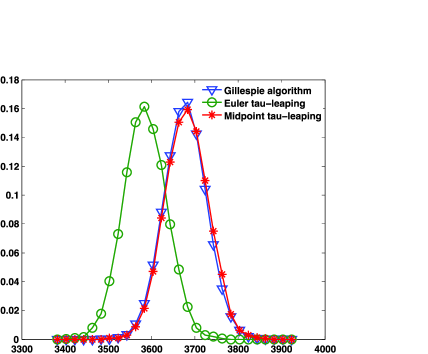
Figure 1: Relative frequency of $X(1)$ from $200\mbox{,}000$ sample paths constructed using (i) Gillespie’s algorithm, blue line $\nabla$ marker, (ii) Euler tau-leaping, green line, $\bigcirc$ marker, and (iii) midpoint tau-leaping, red line, $*$ marker. The approximated distribution generated via midpoint tau-leaping is clearly closer to the exact distribution than that of Euler tau-leaping.

It is simple to show that $X(1)$ is a binomial$(n,p)$ random variable with parameters $n=10\mbox{,}000$ and $p=1/e$. Therefore, $\mathbb{E}X(1)=10\mbox{,}000/e\approx 3678.8$. The estimated means produced from the 200,000 sample paths of Euler tau-leaping and midpoint tau-leaping were $3585.4$ and $3681.4$, respectively. Solving for $\mathcal{E}(t)$ of (3.10) for this example yields $\mathcal{E}(t)=(1/2)e^{-t}t$. Theorem 4.1 therefore estimates that Euler tau-leaping should produce a mean $(1/2)e^{-1}10\mbox{,}000^{1-0.325}\approx 92.2$ smaller than the actual mean, which is in agreement with $3678.8-3585.4=93.4$. Solving for $\mathcal{E}_{1}(t)$ of (41) for this example yields $\mathcal{E}_{1}(t)=(1/6)te^{-t}$. Theorem 4.5 therefore estimates that midpoint tau-leaping should produce a mean $(1/6)e^{-1}10\mbox{,}000^{1-2*0.325}=4.62$ smaller than the actual mean, which is in agreement with $3678.8-3681.4=-2.6$.

Example 5.2.

We now consider a simple Lotka–Volterra predator–prey model. Letting $A$ and $B$ represent the prey and predators, respectively, in a given environment we suppose (i) prey reproduce at a certain rate, (ii) interactions between predators and prey benefit the predator while hurting the prey, and (iii) predators die at a certain rate. One possible model for this system is

$$A\stackrel{{\scriptstyle 2}}{{\rightarrow}}2A,\qquad A+B\stackrel{{\scriptstyle 0.002}}{{\rightarrow}}2B,\qquad B\stackrel{{\scriptstyle 2}}{{\rightarrow}}\varnothing,$$

where a choice of rate constants has been made. Letting $X(t)\in\mathbb{Z}^{2}_{\geq 0}$ be such that $X_{1}(t)$ and $X_{2}(t)$ represent the numbers of prey and predators at time $t>0$, respectively, $X(t)$ satisfies

$$X(t) = X(0)+Y_{1}\biggl{(}\int_{0}^{t}2X_{1}(s)\,ds\biggr{)}\left[\matrix{1\cr 0}\right]$$

$${}+Y_{2}\biggl{(}\int_{0}^{t}0.002X_{1}(s)X_{2}(s)\,ds\biggr{)}\left[\matrix{-1\cr 1}\right]$$

$${}+Y_{3}\biggl{(}\int_{0}^{t}2X_{2}(s)\,ds\biggr{)}\left[\matrix{0\cr-1}\right].$$

We take $X(0)=[1\mbox{,}000,1\mbox{,}000]^{T}$, and so $V=1\mbox{,}000$ for our model. Lotka–Volterra models are famous for producing periodic solutions; this behavior is demonstrated in Figure 2.

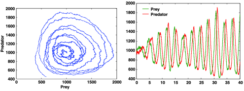
Figure 2: Oscillations in a predator–prey model. In the left image we see the numbers of predators versus the number of prey for a single realization of the system (5.2). In the right image we see the time-series of the numbers of predators and prey for a single realization of (5.2).

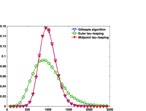
Figure 3: Relative frequency of $X_{2}(10)$ from $30\mbox{,}000$ sample paths constructed using (i) Gillespie’s algorithm, blue line $\nabla$ marker, (ii) Euler tau-leaping, green line, $\bigcirc$ marker, and (iii) midpoint tau-leaping, red line, $*$ marker. The approximated distribution generated via midpoint tau-leaping is clearly closer to the exact distribution than that of Euler tau-leaping.

We approximate the distribution of $X_{2}(10)$ using $30\mbox{,}000$ sample paths constructed using the Gillespie algorithm, Euler tau-leaping with a step-size of $1/20$ and midpoint tau-leaping with a step-size of $1/20$. Note that in this case $1/20=1/V^{0.434}$, and so $\beta=0.434$. The computational results are presented in Figure 3, which again demonstrate the stronger convergence rate of midpoint tau-leaping as compared to Euler tau-leaping.

Appendix

Lemma .1

Let $M$ be a $\{\mathcal{F}_{t}\}$-martingale, $R$ be bounded and $\{\mathcal{F}_{t}\}$-adapted, and let $h>0$. Then for $\eta(t)\equiv[t/h]h$,

$$\hat{M}(t)=\int_{0}^{t}R\circ\eta(s)\bigl{(}M(s)-M\circ\eta(s)\bigr{)}\,ds+R\circ\eta(t)\bigl{(}M(t)-M\circ\eta(t)\bigr{)}\bigl{(}\eta(t)+h-t\bigr{)}$$

is an $\{\mathcal{F}_{t}\}$-martingale and

$$[\hat{M}]_{t}=\int_{0}^{t}\bigl{(}R\circ\eta(r)\bigr{)}^{2}\bigl{(}\eta(r)+h-r\bigr{)}^{2}\,d[M]_{r}.$$ (1)

If $M$ is $\mathbb{R}^{d}$-valued and $R$ is $\mathbb{M}^{m\times d}$-valued, then the quadratic covariation matrix is

$$[\hat{M}]_{t}=\int_{0}^{t}\bigl{(}\eta(r)+h-r\bigr{)}^{2}R\circ\eta(r)\,d[M]_{r}R^{T}\circ\eta(r).$$

For $t<T-h$,

$$\mathbb{E}[\hat{M}(T)|\mathcal{F}_{t}] = \mathbb{E}\biggl{[}\int_{0}^{T}R\circ\eta(s)\bigl{(}M(s)-M\circ\eta(s)\bigr{)}\,ds\big{|}\mathcal{F}_{t}\biggr{]}$$

$$= \mathbb{E}\biggl{[}\int_{0}^{\eta(t)+h}R\circ\eta(s)\bigl{(}M(s)-M\circ\eta(s)\bigr{)}\,ds\big{|}\mathcal{F}_{t}\biggr{]}$$

$$= \int_{0}^{t}R\circ\eta(s)\bigl{(}M(s)-M\circ\eta(s)\bigr{)}\,ds$$

$${}+R\circ\eta(t)\bigl{(}M(t)-M\circ\eta(t)\bigr{)}\bigl{(}\eta(t)+h-t\bigr{)}.$$

The case of $T-h\leq t<T$ is similar. $[\hat{M}]$ is just the quadratic variation of the second term on the right, and noting that $\hat{M}$ is continuous at $t=kh$ for all $k=0,1,2\ldots,$ (1) follows.

For completeness, we include a statement of the martingale central limit theorem (see Kurtz86 for more details).

Lemma .2

Let $\{M_{n}\}$ be a sequence of $\mathbb{R}^{d}$-valued martingales with $M_{n}(0)=0$. Suppose

$$\lim_{n\to\infty}\mathbb{E}\Bigl{[}\sup_{s\leq t}|M_{n}(s)-M_{n}(s-)|\Bigr{]}=0$$

and

$$[M_{n}^{i},M_{n}^{j}]_{t}\to c_{i,j}(t)$$

for all $t\,{>}\,0$ where $C\,{=}\,((c_{i,j}))$ is deterministic and continuous. Then $M_{n}\,{\Rightarrow}\,M$, where $M$ is Gaussian with independent increments and $\mathbb{E}[M(t)M(t)^{T}]=C(t)$.

References

- (1) {barticle}[pbm] \bauthor\bsnmAnderson, \bfnmDavid F.\binitsD. F. (\byear2007). \btitleA modified next reaction method for simulating chemical systems with time dependent propensities and delays. \bjournalJ. Chem. Phys. \bvolume127 \bpages214107. \biddoi=10.1063/1.2799998, pmid=18067349 \endbibitem
- (2) {barticle}[pbm] \bauthor\bsnmAnderson, \bfnmDavid F.\binitsD. F. (\byear2008). \btitleIncorporating postleap checks in tau-leaping. \bjournalJ. Chem. Phys. \bvolume128 \bpages054103. \biddoi=10.1063/1.2819665, pmid=18266441 \endbibitem
- (3) {barticle}[pbm] \bauthor\bsnmCao, \bfnmYang\binitsY., \bauthor\bsnmGillespie, \bfnmDaniel T.\binitsD. T. and \bauthor\bsnmPetzold, \bfnmLinda R.\binitsL. R. (\byear2005). \btitleAvoiding negative populations in explicit Poisson tau-leaping. \bjournalJ. Chem. Phys. \bvolume123 \bpages054104. \biddoi=10.1063/1.1992473, pmid=16108628 \endbibitem
- (4) {barticle}[auto:STB—2010-11-18—09:18:59] \bauthor\bsnmCao, \bfnmYang\binitsY., \bauthor\bsnmGillespie, \bfnmDaniel T.\binitsD. T. and \bauthor\bsnmPetzold, \bfnmLinda R.\binitsL. R. (\byear2006). \btitleEfficient step size selection for the tau-leaping simulation method. \bjournalJ. Chem. Phys. \bvolume124 \bpages044109. \endbibitem
- (5) {barticle}[pbm] \bauthor\bsnmChatterjee, \bfnmAbhijit\binitsA., \bauthor\bsnmVlachos, \bfnmDionisios G.\binitsD. G. and \bauthor\bsnmKatsoulakis, \bfnmMarkos A.\binitsM. A. (\byear2005). \btitleBinomial distribution based tau-leap accelerated stochastic simulation. \bjournalJ. Chem. Phys. \bvolume122 \bpages024112. \biddoi=10.1063/1.1833357, pmid=15638577 \endbibitem
- (6) {bbook}[mr] \bauthor\bsnmEthier, \bfnmStewart N.\binitsS. N. and \bauthor\bsnmKurtz, \bfnmThomas G.\binitsT. G. (\byear1986). \btitleMarkov Processes: Characterization and Convergence. \bpublisherWiley, \baddressNew York. \biddoi=10.1002/9780470316658, mr=0838085 \endbibitem
- (7) {bbook}[mr] \bauthor\bsnmEthier, \bfnmStewart N.\binitsS. N. and \bauthor\bsnmKurtz, \bfnmThomas G.\binitsT. G. (\byear2005). \btitleMarkov Processes: Characterization and Convergence, \bedition2nd ed. \bpublisherWiley, \baddressNew York. \endbibitem
- (8) {barticle}[auto:STB—2010-11-18—09:18:59] \bauthor\bsnmGibson, \bfnmM. A.\binitsM. A. and \bauthor\bsnmBruck, \bfnmJ.\binitsJ. (\byear2000). \btitleEfficient exact stochastic simulation of chemical systems with many species and many channels. \bjournalJ. Phys. Chem. A \bvolume105 \bpages1876–1889. \endbibitem
- (9) {barticle}[mr] \bauthor\bsnmGillespie, \bfnmDaniel T.\binitsD. T. (\byear1976). \btitleA general method for numerically simulating the stochastic time evolution of coupled chemical reactions. \bjournalJ. Comput. Phys. \bvolume22 \bpages403–434. \bidmr=0503370 \endbibitem
- (10) {barticle}[auto:STB—2010-11-18—09:18:59] \bauthor\bsnmGillespie, \bfnmD. T.\binitsD. T. (\byear1977). \btitleExact stochastic simulation of coupled chemical reactions. \bjournalJ. Phys. Chem. \bvolume81 \bpages2340–2361. \endbibitem
- (11) {barticle}[auto:STB—2010-11-18—09:18:59] \bauthor\bsnmGillespie, \bfnmD. T.\binitsD. T. (\byear2001). \btitleApproximate accelerated simulation of chemically reaction systems. \bjournalJ. Chem. Phys. \bvolume115 \bpages1716–1733. \endbibitem
- (12) {barticle}[auto:STB—2010-11-18—09:18:59] \bauthor\bsnmGillespie, \bfnmD. T.\binitsD. T. and \bauthor\bsnmPetzold, \bfnmLinda R.\binitsL. R. (\byear2003). \btitleImproved leap-size selection for accelerated stochastic simulation. \bjournalJ. Chem. Phys. \bvolume119 \bpages8229–8234. \endbibitem
- (13) {bbook}[mr] \bauthor\bsnmKloeden, \bfnmPeter E.\binitsP. E. and \bauthor\bsnmPlaten, \bfnmEckhard\binitsE. (\byear1992). \btitleNumerical Solution of Stochastic Differential Equations. \bseriesApplications of Mathematics (New York) \bvolume23. \bpublisherSpringer, \baddressBerlin. \bidmr=1214374 \endbibitem
- (14) {barticle}[auto:STB—2010-11-18—09:18:59] \bauthor\bsnmKurtz, \bfnmThomas G.\binitsT. G. (\byear1972). \btitleThe relationship between stochastic and deterministic models for chemical reactions. \bjournalJ. Chem. Phys. \bvolume57 \bpages2976–2978. \endbibitem
- (15) {barticle}[mr] \bauthor\bsnmKurtz, \bfnmThomas G.\binitsT. G. (\byear1977/78). \btitleStrong approximation theorems for density dependent Markov chains. \bjournalStochastic Processes Appl. \bvolume6 \bpages223–240. \bidmr=0464414 \endbibitem
- (16) {bbook}[mr] \bauthor\bsnmKurtz, \bfnmThomas G.\binitsT. G. (\byear1981). \btitleApproximation of Population Processes. \bseriesCBMS-NSF Regional Conference Series in Applied Mathematics \bvolume36. \bpublisherSIAM, \baddressPhiladelphia, PA. \bidmr=0610982 \endbibitem
- (17) {barticle}[mr] \bauthor\bsnmLi, \bfnmTiejun\binitsT. (\byear2007). \btitleAnalysis of explicit tau-leaping schemes for simulating chemically reacting systems. \bjournalMultiscale Model. Simul. \bvolume6 \bpages417–436 (electronic). \biddoi=10.1137/06066792X, mr=2338489 \endbibitem
- (18) {barticle}[mr] \bauthor\bsnmRathinam, \bfnmMuruhan\binitsM., \bauthor\bsnmPetzold, \bfnmLinda R.\binitsL. R., \bauthor\bsnmCao, \bfnmYang\binitsY. and \bauthor\bsnmGillespie, \bfnmDaniel T.\binitsD. T. (\byear2005). \btitleConsistency and stability of tau-leaping schemes for chemical reaction systems. \bjournalMultiscale Model. Simul. \bvolume4 \bpages867–895 (electronic). \biddoi=10.1137/040603206, mr=2203944 \endbibitem
- (19) {bbook}[mr] \bauthor\bsnmWilkinson, \bfnmDarren James\binitsD. J. (\byear2006). \btitleStochastic Modelling for Systems Biology. \bpublisherChapman and Hall/CRC, \baddressBoca Raton, FL. \bidmr=2222876 \endbibitem