Exact Calculation of Entanglement in a 19-site 2D Spin System

Abstract

Using the Trace Minimization Algorithm, we carried out an exact calculation of entanglement in a 19-site two-dimensional transverse Ising model. This model consists of a set of localized spin-$\frac{1}{2}$ particles in a two dimensional triangular lattice coupled through exchange interaction $J$ and subject to an external magnetic field of strength $h$. We demonstrate, for such a class of two-dimensional magnetic systems, that entanglement can be controlled and tuned by varying the parameter $\lambda=h/J$ in the Hamiltonian and by introducing impurities into the systems. Examining the derivative of the concurrence as a function of $\lambda$ shows that the system exhibits a quantum phase transition at about $\lambda_{c}=3.01$, a transition induced by quantum fluctuations at the absolute zero of temperature.

I Introduction

Entanglement, which is a quantum mechanical property that has no classical analog, has been viewed as a resource of quantum information and computation amico2008 ; diviccezo ; entg1 ; Nielsen ; gruska ; vedral ; nori1 ; nori2 . Intensive researches of entanglement measurement, entanglement monotone, criteria for distinguishing separable from entangled pure states and all the extensions from bipartite to multipartite systems have been carried out both qualitatively and quantitatively amico2008 . At the interface between quantum information and statistical mechanics, there has been particular analysis of entanglement in quantum critical models osterloh ; osborne ; osterloh2004 ; vidal2003 .

The critical properties in the entanglement allow for a screening of the qualitative change of the system and a deeper characterization of the ground state wavefunction undergoing a phase transition. At T=0, ground states of many-body systems contain all correlations concerning phases of matters. Traditionally, systems have been studied by looking, for example, at their external perturbations, various order parameters and excitation spectrum amico2008 . Methods developed from quantum information shed light on new ways of studying many-body systems Lidar1 ; Lidar2 ; Lidar3 ; Lidar4 , such as providing support for numerical calculations, like density matrix renormalization or design of new efficient simulation strategies for many-body systems.

Entanglement close to quantum phase transitions was originally analyzed by Osborne and Nielsen osborne , and Osterloh et al. osterloh for the Ising model in one dimension. Recently, we studied a set of localized spins coupled through exchange interaction and subject to an external magnetic filed Osenda1 ; Osenda2 ; Osenda3 ; Osenda4 . We demonstrated for such a class of one-dimensional magnetic systems, that entanglement can be controlled and tuned by varying the anisotropy parameter in the Hamiltonian and by introducing impurities into the systems. In particular, under certain conditions, the entanglement is zero up to a critical point $\lambda_{c}$, where a quantum phase transition occurs, and is different from zero above $\lambda_{c}$ kais2002 .

In two and higher dimensions nearly all calculations for spin systems were obtained by means of numerical simulations Sandvik1 ; Sandvik2 . The concurrence and localizable entanglement in two-dimensional quantum XY and XXZ models were considered using quantum Monte Carlo Syluasen1 ; Syluasen2 . The results of these calculations were qualitatively similar to the one-dimensional case, but entanglement is much smaller in magnitude. Moreover, the maximum in the concurrence occurs at a position closer to the critical point than in the one-dimensional case amico2008 .

The Trace Minimization Algorithm for Hermitian eigenvalue problems, like those under consideration in this paper, was introduced in 1982 by A. Sameh and J. Wisniewski sameh1982 . It was designed specifically to handle very large problems on parallel computing platforms for obtaining the smallest eigenpairs. Later, a similar algorithm (Jacobi-Davidson) for the same eigenvalue problem was introduced by Sleijpen and Van der Vorst in 1996. A comparison of the two schemes by A. Sameh and Z. Tong in 2000 sameh2000 showed that the Trace Minimization scheme is more robust and efficient Sleijen .

In this paper, we use the Trace Minimization Algorithm sameh1982 ; sameh2000 to carry out an exact calculation of entanglement in a 19-site two dimensional transverse Ising model. We classify the ground state properties according to its entanglement for certain class on two-dimensional magnetic systems and demonstrate that entanglement can be controlled and tuned by varying the parameter $\lambda=h/J$ in the Hamiltonian and by introducing impurities into the systems. The paper is organized as follows. In the next section, we give a brief overview of the model, entanglement of formation and the trace minimization algorithm. Detailed methods are addressed in the appendix. We then proceed with the results and discussions of 1. the calculation of exact entanglement of a 19-site spin system, 2. the relationship of entanglement and quantum phase transition, and 3. the effects of impurities on the entanglement. The conclusions and the outlook are presented in the concluding section.

II Method

II.1 Model

We consider a set of localized spin-$\frac{1}{2}$ particles in a two dimensional triangular lattice coupled through exchange interaction $J$ and subject to an external magnetic field of strength $h$. The Hamiltonian for such a system is given by

$$H=-\sum_{<i,j>}J_{i,j}\sigma_{i}^{x}\sigma_{j}^{x}-h\sum_{i}\sigma_{i}^{z},$$ (1)

where $<i,j>$ is a pair of nearest-neighbors sites on the lattice, $J_{i,j}=J$ for all sites except the sites nearest to the impurity site $i_{m}$, while around the impurity site $J_{i,j}=(1+\alpha)J$, $\alpha$ measures the strength of the impurity which is located at site $i_{m}$, and $\sigma_{i}^{x}$ and $\sigma_{i}^{z}$ are the Pauli matrices. For this model it is convenient to define a dimensionless coupling constant $\lambda=h/J$.

II.2 Entanglement of formation

We confine our interest to the entanglement of two spins, at any position $i$ and $j$ osterloh . We adopt the entanglement of formation, a well known measure of entanglement wooters1998 , to quantify our entanglement kais2002 . All the information needed in this case is contained in the reduced density matrix $\rho_{i,j}$. Wootters wooters1998 has shown, for a pair of binary qubits, that the concurrence $C$, which goes from $0$ to $1$, can be taken as a measure of entanglement. The concurrence between sites $i$ and $j$ is defined as wooters1998

$$C(\rho)=max\{0,\epsilon_{1}-\epsilon_{2}-\epsilon_{3}-\epsilon_{4}\},$$ (2)

where the $\epsilon_{i}$’s are the eigenvalues of the Hermitian matrix $R\equiv\sqrt{\sqrt{\rho}\tilde{\rho}\sqrt{\rho}}$ with $\tilde{\rho}=(\sigma^{y}\otimes\sigma^{y})\rho^{*}(\sigma^{y}\otimes\sigma^{y})$ and $\sigma^{y}$ is the Pauli matrix of the spin in y direction. For a pair of qubits the entanglement can be written as,

$$E(\rho)=\epsilon(C(\rho)),$$ (3)

where $\epsilon$ is a function of the “concurrence” $C$

$$\epsilon(C)=h\left(\frac{1-\sqrt{1-C^{2}}}{2}\right),$$ (4)

where $h$ is the binary entropy function

$$h(x)=-x\log_{2}x-(1-x)log_{2}(1-x).$$ (5)

In this case, the entanglement of formation is given in terms of another entanglement measure, the concurrence C. The entanglement of formation varies monotonically with the concurrence.

The matrix elements of the reduced density matrix needed for calculating the concurrence are obtained numerically using the formalism developed in the following section.

II.3 Trace minimization algorithm (Tracemin)

Diagonalizing a $2^{19}$ by $2^{19}$ Hamiltonian matrix and partially tracing its density matrix is a numerically difficult task. We propose to compute the entanglement of formation, first by applying the trace minimization algorithm (Tracemin) sameh1982 ; sameh2000 to obtain the eigenvalues and eigenvectors of the constructed Hamiltonian. Then, we use these eigenpairs and new techniques detailed in the appendix to build partially traced density matrix.

The trace minimization algorithm was developed for computing a few of the smallest eigenvalues and the corresponding eigenvectors of the large sparse generalized eigenvalue problem

$$AU=BU\Sigma,$$ (6)

where matrices $A,B\in\mathbb{C}^{n\times n}$ are Hermitian positive definite, $U=[u_{1},...,u_{p}]\in\mathbb{C}^{n\times p}$ and $\Sigma\in\mathbb{R}^{p\times p}$ is a diagonal matrix. The main idea of Tracemin is that minimizing $Tr(X^{*}AX)$, subject to the constraints $X^{*}BX=I$, is equivalent to finding the eigenvectors $U$ corresponding to the p smallest eigenvalues. This consequence of Courant-Fischer Theorem can be restated as

$$\min_{X^{*}BX=I}Tr(X^{*}AX)=Tr(U^{*}AU)=\sum_{i=1}^{p}\lambda_{i},$$ (7)

where $I$ is the identity matrix. The following steps constitute a single iteration of the Tracemin algorithm:
$\bullet\quad G=X_{k}^{*}BX_{k}$ (compute $G$) $\bullet\quad G=V\Omega V^{*}$ (compute the spectral decomposition of $G$) $\bullet\quad H=\tilde{Q}^{*}A\tilde{Q}$ (compute $H$, where $\tilde{Q}=X_{k}V\Omega^{-1/2}$) $\bullet\quad H=W\Omega W^{*}$ (compute the spectral decomposition of $H$) $\bullet\quad\bar{X}_{k}=\tilde{Q}W$ (now $\bar{X}_{k}^{*}A\bar{X}_{k}=\Lambda$ and $\bar{X}_{k}^{*}B\bar{X}_{k}=I$) $\bullet\quad\bar{X}_{k+1}=\bar{X}_{k}-D$ ( $D$ is determined s.t. $Tr(X_{k+1}^{*}AX_{k+1})<Tr(X_{k}^{*}AX_{k})$ ).
In order to find the optimal update $D$ in the last step, we enforce the natural constraint $\bar{X}_{k}^{*}BD=0$, and obtain

$$\begin{pmatrix}A&B\bar{X}_{k}\\ X_{k}^{*}B&0\end{pmatrix}\begin{pmatrix}D\\ L\end{pmatrix}=\begin{pmatrix}A\bar{X}_{k}\\ 0\end{pmatrix}$$ (8)

.

Considering the orthogonal projector $P=B\bar{X}_{k}(X_{k}^{*}B^{2}X_{k})^{-1}\bar{X}_{k}^{*}B$ and letting $D=(I-P)\bar{D}$, the linear system (8) can be rewritten in the following form

$$(I-P)A(I-P)\bar{D}=(I-P)A\bar{X}_{k}.$$ (9)

Notice that the Conjugate Gradient method can be used to solve (9), since it can be shown that the residual and search directions $\text{r},\text{p}\in\text{Range}(P)^{\perp}$. Also, notice that the linear system (9) need to be solved only to a fixed relative precision at every iteration of Tracemin.

A reduced density matrix, built from the ground state which is obtained by Tracemin, is usually constructed as follows: diagonalize the system Hamiltonian $H(\lambda)$, retrieve the ground state $|\Psi>$ as a function of $\lambda=h/J$, build the density matrix $\rho=|\Psi><\Psi|$, and trace out contributions of all the other spins in density matrix to get reduced density matrix by $\rho(i,j)=\sum_{p}<u_{i}(A)|<v_{p}(B)|\rho|u_{j}(A)>|v_{p}(B)>$, where ${u_{i}(A)}$ and ${v_{p}(B)}$ are bases of subspaces $\epsilon(A)$ and $\epsilon(B)$. That includes creating a $2^{19}\times 2^{19}$ density matrix $\rho$ followed by permutations of rows, columns and some basic arithmetic operations on the elements of $\rho$. Instead of operating on a huge matrix, we pick up only certain elements from $|\Psi>$, performing basic algebra to build a reduced density matrix directly. Details are in the Appendix.

III Results and discussions

III.1 Exact entanglement of a 19-site spin system

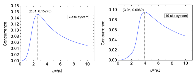
Figure 1: (Color online) Concurrence of center spin and its nearest neighbor as a function of $\lambda$ for both 7-site and 19-site system. In the 7-site system, concurrence reaches maximum 0.15275 when $\lambda=2.61$. In the 19-site system, concurrence reaches the maximum 0.0960 when $\lambda=3.95$.

We examine the change of concurrence in Eq. (2) between the center spin and its nearest neighbor as a function of $\lambda=h/J$ for both the 7-site and 19-site systems. In Fig.1, the concurrence of the 7-site system reaches its maximum 0.15275 when $\lambda=2.61$. In the 19-site system, the concurrence reaches 0.0960 when $\lambda=3.95$. The maximum value of concurrence in the 19-site model, where each site interacts with six neighbors, is roughly 1/3 of the maximum concurrence in the one-dimensional transverse Ising model with size N=201 Osenda1 , where it has only two neighbors for each site. It is the monogamy Coffman ; osborne2006 that limits the entanglement shared among the number of neighboring sites.

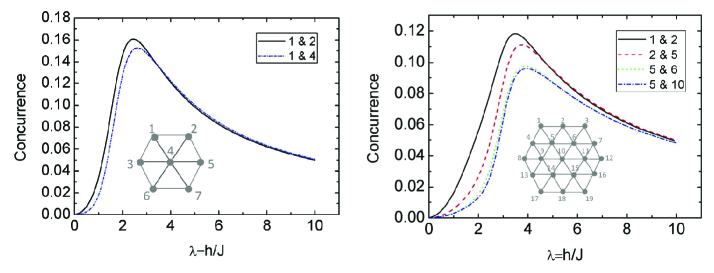
Figure 2: (Color online) The nearest neighbor concurrence as a function of $\lambda$ for different pairs. In 7-site system, there are two distinct pairs $1\ \&\ 2$ and $1\ \&\ 4$. In 19-site system, they are $1\ \&\ 2$, $2\ \&\ 5$, $5\ \&\ 6$ and $5\ \&\ 10$.

However, entanglement between other nearest neighbors are slightly different than those between the pairs involving the center. Figure 2 shows that the less the number of neighbors of a pair the larger the entanglement. The concurrence between the 1st and 2nd spins is greater than that between the 1st and 4th in the 7-site system. For the 19-site one, the concurrence between the 1st and 2nd spins is greater than that between the 2nd and 5th. The same rule applies to the others, therefore $C_{2,5}>C_{5,6}>C_{5,10}$. Although $5\ \&\ 6$ and $5\ \&\ 10$ have the same number of neighbors, the number of neighbors of neighbors of $5\ \&\ 6$ is less than that of $5\ \&\ 10$. Consequently, $C_{5,6}$ is slightly larger than $C_{5,10}$.

Our numerical calculation shows that the maximum concurrence of next nearest neighbor (say the 1st and 10th spins) is less than $10^{-8}$. The truly non-local quantum part of the two-point correlations is nonetheless very short-rangedosterloh . It shows that the entanglement is short ranged, though global. These results are similar to those obtained for Ising one-dimensional spin systems in a transverse magnetic fieldosterloh . The range of entanglement, that is the maximum distance between two spins at which the concurrence is different from zero, is short. The concurrence vanishes unless the two sites are at most next-neighbours.

III.2 Entanglement and quantum phase transition

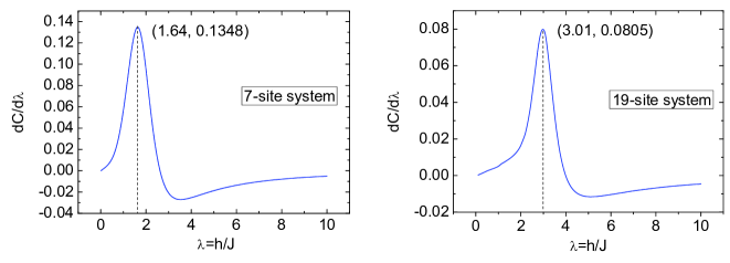
Figure 3: (Color online) The change of concurrence between the center and its nearest neighbor as a function of parameter $\lambda$ for 7-site and 19-site systems respectively. They both show the strong tendency of singularity at $\lambda=1.54$ and $\lambda=3.01$.

As we mentioned in Part II-B, all the information needed for quantifying the entanglement of two spins is contained in the reduced density matrix obtained from density matrix. In other words, entanglement is coded by the information of ground state, while the quantum phase transition is characterized by the change of ground state. In order to quantify the change of the many-body wavefunction when the system crosses the critical point, we calculate the change of concurrence $dC/d\lambda$ between the center and its nearest neighbor as a function of parameter $\lambda$ for both 7 and 19 sites systems, as shown in Fig.3. It is known that an infinite system, a system is at the thermodynamic limit, is supposed to have a singularity at the critical point of quantum phase transition; for a finite system one still has to take finite size effect into consideration. However, in Fig.3 both systems show strong tendency of being singular at $\lambda_{c}=1.64$ and $\lambda_{c}=3.01$ respectively. Renormalization group method for an infinite triangular system predicts critical point at $\lambda_{c}=4.75784$; the same method for a square lattice system at $\lambda_{c}=2.62975$ Penson , while finite-size scaling has $\lambda_{c}=3.044$ for square lattice Hamer . Our results show that the tendency to be singular is moving towards the infinite critical point as the size increases. For one-dimensional system since the calculations can be done for large number of spins, finite size scaling calculations for N ranging from 41 to 401 spins indicate that the derivative of the concurrence diverges logarithmically with increasing system size osterloh . In our study we can not perform finite size scaling analysis since we do not have enough data points to perform data collapse Kais-Review . Optimization methodsKais-Opt and Parallel Tracemin code is under development which will allow us to obtain exact results for larger system.

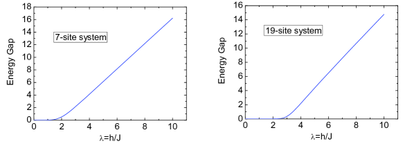
Figure 4: (Color online) The energy separation between the ground state and the first excited state as a function of $\lambda$.

To understand this model better, a discussion about the degeneracy in the system and an explanation of the energy spectrum is necessary. It is known that the ground state degeneracy of the Heisenberg spin model depends on whether the total number of spins is even (singlet) or odd (doublet). For the Ising model with transverse field on an infinite 1D chain, the ground state in the ferromagnetic (FM) phase is doubly degenerate and is gaped from the excitation spectrum by $2J(1-h/J)$ sachdev . (Note that, however, this degeneracy is never achieved unless one goes to the thermaldynamic limit, regardless number of spins being even or odd.) In our model, the Ising coupling is ferromagnetic, as opposed to the spin liquid case with antiferromagnetic coupling, the system is expected to break the $Z_{2}$ symmetry and develop the (Ising) FM order under small transverse field. Further, due to the construction of the lattice, it is impossible to have a system that has even number of sites while conserving all the lattice group symmetries. So we expect that the same doublet degeneracy remains in 2D as the system goes to the thermaldynamic limit. The energy gaps from our numerical results of finite systems are less than $10^{-8}$ (Fig.4), which are well consistent with the expectation. The strict doublets in finite systems only happen at $h/J=0$ exactly, when entanglements naturally are zero, not entangled at all; no matter which one of the doublet ground state is chosen, it gives the same value of entanglement. Otherwise even very small h help distinguish the ground state. Technically we don’t have to worry about that a different superposition of the ground states gives different values of entanglement.

The energy separation between the ground state and the first excited state in terms of $\lambda$ clarifies the spectrum of the system. Figure 4 presents the doubly degeneracy of the ground state and they separate around $\lambda=1.5$ for the 7-site and $\lambda=2.5$ for the 19-site system. While in the $dC/d\lambda$ vs $\lambda$ graph, both systems show strong tendency of being singular at $\lambda_{c}=1.64$ and $\lambda_{c}=3.01$ respectively. Both “separation position” and “singular position” are used as an indicator of “critical point”. And we believe using the finite-size scaling both will give the same “critical point” of the infinite system. But it seems $dC/d\lambda$ vs $\lambda$ is a better indicator because for the same size system it points out a value closer to the expected critical point. This property benefits the finite size scaling method, since less/smaller systems may be needed.

III.3 Introducing impurities to tune the entanglement

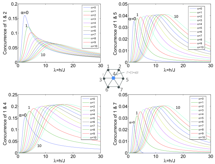
Figure 5: (Color online) Concurrences of different pairs with various strength of impurity in the center of the 7-site system.

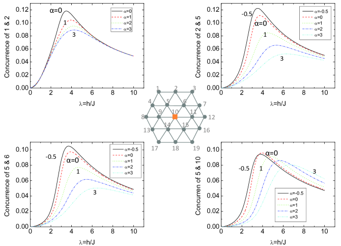
Figure 6: (Color online) Concurrence of different pairs with various strength of impurity in the center of the 19-site system.

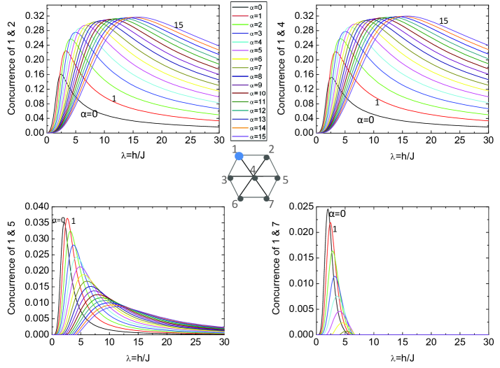
Figure 7: (Color online) Concurrence of different pairs with various strength of impurity at site 1 of a 7-site system.

We introduce one impurity in the center of the 19-site spin system. The impurity only interacts with nearest neighbors in strength $J^{\prime}=(1+\alpha)J$. When the strength increases, the concurrence of any two spins decreases. Then we move the impurity to site 5. The concurrence shows the same trend of decreasing, as the impurity strengths go up. Details are shown in Fig.5 for the concurrence of different pairs with various strength of impurity in the center of the 7-site system, while Fig.6 show the results for 19-site system. Fig.7 shows the results with various strength of impurity at site 1 of a 7-site system and Fig.8 for various strength of impurity at site 5 of a 19-site system.

The maximum of entanglement is shifted with the increasing of the parameter $\alpha$. The shift is the result of the competition between the spin-spin interaction $J$ and the external transverse magnetic field $h$. Consider the ideal situation of pure infinite system. Without the coupling interaction, all the spins will point along the direction of transverse field. While with the absence of transverse field, the ground state is supposed to be 2-fold degenerated, either along the positive x direction or the negative x direction. Every spin has six neighbors, so averagely is affected by three $J$, and one $h$. When the two forces are well-matched in strength, the phase transition occurs. Fig. 3 indicates the 19-site system has strong tendency of singularity at $\lambda=3.01$, which is consistent and very close with the above statement. When the system is finite, the boundary effect (less than six neighbors) will affect the position of the maximum of entanglement a little bit as Fig. 2 shows for different pairs. After we introduce the impurity, the balance of $3:1$ is destroyed, so the the maximum of entanglement is shifted quite a bit for different strength of $J^{\prime}=(1+\alpha)J$.

The value of the maximum changes with $\alpha$ is because of the monogamy that limits the entanglement shared among neighbors. For example, in Fig. 4, the stronger the interactions between 1 $\&$ 4 and 2 $\&$ 4, i.e. the larger $\alpha$, the less 1 $\&$ 2 entangle. So the value of maximum goes down for larger $\alpha$.

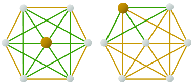
Figure 9: (Color online) Overview of the change of concurrence in 7-site system. The large yellow dot stands for the impurity and silver dots denote regular spins. Lines connecting two sites represent the entanglement. If the line is green, it means the entanglement between two sites increases as the impurity gets “stronger”, otherwise the yellow line indicates that the entanglement decrease when the impurity increases.

Figure 9 gives a good overview of the change of concurrence for the 7-site system. The large yellow dot stands for the impurity and silver dots denote regular spins. Lines connecting two sites represent the entanglement. If the line is green, it means the entanglement between two sites increases as the impurity gets “stronger”, and the yellow line indicates that the entanglement decreases when the impurity increases. We can explain these phenomena of 7-site system as follows. When the impurity interacts more with the neighbor, the pair also entangles more. Since some spins are more involved with the impurity, they themselves entangle less. The only exceptions are the next nearest neighbors. Thus, entanglement close to the impurity tends to get bigger when J’ is greater than J. However, the behavior of entanglement between site 5 and 10 in the 19-site system surprisingly goes down as the strength of the impurity coupling increases. It is not clear why the behavior is different for the one in the 7-site system and whether increasing the system size has any effect. We are planing to increase the size of the system to include the next layer, which will bring the system to 37-site, in order to analyze this phenomena.

All the results above are obtained through sequential computing. In the future to increase the object size under consideration, we plan to take advantage of parallel computing. We already have a parallel Tracemin algorithm and we are developing a parallel code for computation of the partial trace. This will be useful as we expand our 2D systems to larger number of spins in order to perform finite-size scaling for quantum critical parameters.

In summary, the Tracemin algorithm allowed us to carry out an exact calculation of entanglement in a 19-site two dimensional transverse Ising model. We demonstrated for such a class of two-dimensional magnetic systems, that entanglement can be controlled and tuned by varying the parameter $\lambda$ in the Hamiltonian and by introducing impurities into the systems.

IV Acknowledgments

We would like to thank the Army Research Office (ARO) and the BSF for financial support.

Appendix A Applications of trace minimization algorithm

A.1 General forms of matrix representation of the Hamiltonian

By studying the patterns of $\sum_{<i,j>}I\otimes\cdots\sigma_{i}^{x}\otimes\cdots\sigma_{j}^{x}\otimes\cdots I$ and $\sum_{i}I\otimes\cdots\sigma_{i}^{z}\otimes\cdots I$, one founds the following rules.

A.1.1 $\sum_{i}\sigma_{i}^{z}$ for N spins

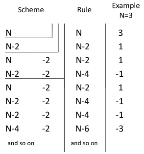
Figure 10: Diagonal elements of $\sum_{i}\sigma_{i}^{z}$ for N spins.

The matrix is $2^{N}$ by $2^{N}$; it has only $2^{N}$ diagonal elements. Elements follow the rules shown in Fig. 10.

If one stores these numbers in a vector, and initializes $v=(N)$, then the new v is the concatenation of the original v and the original v with 2 subtracted from each of its elements. We repeat this N times, i.e.,

$$v=\left(\begin{array}[]{c}v\\ v-2\\ \end{array}\right);$$ (10)

$$v =\left(\begin{array}[]{c}N\end{array}\right),$$ (12)

$$\Rightarrow v =\left(\begin{array}[]{c}N\\ N-2\\ \end{array}\right),$$ (15)

$$\Rightarrow v =\left(\begin{array}[]{c}N\\ N-2\\ N-2\\ N-4\\ \end{array}\right).$$ (20)

A.1.2 $\sum_{<i,j>}I\otimes\cdots\sigma_{i}^{x}\otimes\cdots\sigma_{j}^{x}\otimes\cdots I$ for N spins

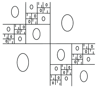
Figure 11: Scheme of matrix $I\otimes\sigma_{3}^{x}\otimes\sigma_{2}^{x}\otimes I\otimes I$

Since $\left(\begin{array}[]{ccc}1&0\\ 0&1\\ \end{array}\right)$ & $\left(\begin{array}[]{ccc}0&1\\ 1&0\\ \end{array}\right)$ exclude each other, for matrix $I\otimes\cdots\sigma_{i}^{x}\otimes\cdots\sigma_{j}^{x}\otimes\cdots I$, every row/column contains only one “1”, then the matrix owns $2^{N}$ “1”s and only “1” in it. If we know the position of “1”s, it turns out that we can set a $2^{N}$ by 1 array “col” to store the column position of “1”s corresponding to the 1st $\rightarrow$ $2^{N}$th rows. In fact, the non-zero elements can be located by the properties stated below. For clarity, let us number N spins in the reverse order as: N-1, N-2, …, 0, instead of 1, 2, …, N. The string of non-zero elements starts from the first row at: $1+2^{i}+2^{j}$; with string length $2^{j}$; and number of such strings $2^{N-j-1}$. For example, Fig. 11 shows these rules for a scheme of $I\otimes\sigma_{3}^{x}\otimes\sigma_{2}^{x}\otimes I\otimes I$.

Again, because of the exclusion, the positions of non-zero element “1” of $I\otimes\cdots\sigma_{i}^{x}\otimes\cdots\sigma_{j}^{x}\otimes\cdots I$ are different from those of $I\otimes\cdots\sigma_{l}^{x}\otimes\cdots\sigma_{m}^{x}\otimes\cdots I$. So $\sum_{<i,j>}I\otimes\cdots\sigma_{i}^{x}\otimes\cdots\sigma_{j}^{x}\otimes\cdots I$ is a $2^{N}$ by $2^{N}$ matrix with only 1 and 0.

After storing array “col”, we repeat the algorithm for all the nearest pairs $<i,j>$, and concatenate “col”s to position matrix “c” of $\sum_{<i,j>}I\otimes\cdots\sigma_{i}^{x}\otimes\cdots\sigma_{j}^{x}\otimes\cdots I$. In the next section we apply these rules to our problem.

A.2 Specialized matrix multiplication

Using the diagonal elements array “v” of $\sum_{i}\sigma_{i}^{z}$ and position matrix of non-zero elements “c” for $\sum_{<i,j>}I\otimes\cdots\sigma_{i}^{x}\otimes\cdots\sigma_{j}^{x}\otimes\cdots I$, we can generate matrix H, representing the Hamiltonian. However, we only need to compute the result of the matrix-vector multiplication H*Y in order to run Tracemin, which is the advantage of Tracemin, and consequently do not need to explicitly obtain H. Since matrix-vector multiplication is repeated many times throughout iterations, we propose an efficient implementation to speedup its computation specifically for Hamiltonian of Ising model (and XY by adding one term).

For simplicity, first let Y in H*Y be a vector and $J=h=1$ (in general Y is a tall matrix and $J\neq h\neq 1$). Then

$$H*Y$$ (42)

$$= \sum_{<i,j>}\sigma_{i}^{x}\sigma_{j}^{x}*Y+\sum_{i}\sigma_{i}^{z}*Y$$

$$= \left(\begin{array}[]{cccccc}1&&1&&1&\\ &1&&1&&1\\ &\ldots&&\ldots&&\\ &&&&&\\ &\ldots&&\ldots&&\\ 1&&&&1&1\\ \end{array}\right)*\left(\begin{array}[]{c}Y(1)\\ Y(2)\\ \vdots\\ \vdots\\ Y(2^{N})\\ \end{array}\right)+\left(\begin{array}[]{ccccc}v(1)&&&&\\ &v(2)&&&\\ &&\ddots&&\\ &&&\ddots&\\ &&&&v(2^{N})\\ \end{array}\right)*\left(\begin{array}[]{c}Y(1)\\ Y(2)\\ \vdots\\ \vdots\\ Y(2^{N})\\ \end{array}\right)$$

$$= \left(\begin{array}[]{c}Y(c(1,1))+Y(c(1,2))+\ldots+Y(c(1,\#ofpairs)\\ \vdots\\ Y(c(k,1))+Y(c(k,2))+\ldots+Y(c(k,\#ofpairs)\\ \vdots\\ Y(c(2^{N},1))+Y(c(2^{N},2))+\ldots+Y(c(2^{N},\#ofpairs)\\ \end{array}\right)+\left(\begin{array}[]{c}v(1)*Y(1)\\ v(2)*Y(2)\\ \vdots\\ \vdots\\ v(2^{N})*Y(2^{N})\end{array}\right),$$ (53)

where p# stands for the number of pairs.

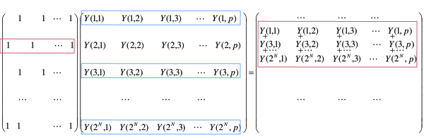
Figure 12: (Color online) The illustration of H*Y.

When Y is a matrix, we can treat Y ($2^{N}$ by p) column by column for $\sum_{<i,j>}I\otimes\cdots\sigma_{i}^{x}\otimes\cdots\sigma_{j}^{x}\otimes\cdots I$. Also, we can accelerate the computation by treating every row of Y as a vector and adding these vectors at once. Fig. 12 visualized the process.

Notice that the result of the multiplication of the xth row of $\sum_{<i,j>}\sigma_{i}^{x}\sigma_{j}^{x}$ (delineated by the red box above) and Y, is equivalent to the sum of rows of Y, whose row numbers are the column indecis of non-zero elements’ of the xth row. Such that we transform a matrix operation to straight forward summation & multiplication of numbers.

Appendix B Partial Trace

All the information needed for quantifying the entanglement of two spins $i$ & $j$ is contained in the reduced density matrix $\rho(i,j)$, which can be obtained from global density matrix $\rho=|\psi\rangle\langle\psi|$, where $|\psi\rangle$ is the ground state of the system, via partial trace. Now let us show how we can obtain the reduced density matrix from the ground state calculated by Tracemin.

B.1 Density operator in the pure case and partial trace

Consider a system whose state vector at the instant $t$ is

$$|\psi(t)\rangle=\sum_{n}c_{n}(t)|u_{n}\rangle,\quad\sum_{n}|c_{n}(t)|^{2}=1.$$ (54)

The density operator $\rho(t)$ is defined as

$$\rho(t)=|\psi(t)\rangle\langle\psi(t)|.$$ (55)

It enables us to obtain all the physical predictions of an observable A(t) by

$$\langle A(t)\rangle=Tr\{\rho(t)A\}.$$ (56)

Let us consider two different system (1) and (2) and the global system (1)+(2), whose state space is the tensor product: $\varepsilon=\varepsilon(1)\otimes\varepsilon(2)$. Let $|u_{n}(1)\rangle$ be a basis of $\varepsilon(1)$ and $|v_{p}(2)\rangle$, a basis of $\varepsilon(2)$, the kets $|u_{n}(1)\rangle|v_{p}(2)\rangle$ from a basis of $\varepsilon$.

The density operator $\rho$ of the global system is an operator which acts in $\varepsilon$. We construct from $\rho$ an operator $\rho(1)$ [or $\rho(2)$] acting only in $\varepsilon(1)$ [or $\varepsilon(2)$] which will enable us to make all the physical prediction about measurements bearing only on system(1) or system(2). This operation will be called a partial trace with respect to (2) [or (1)]. Matrix elements of the operator $\rho(1)$ are

$$\langle u_{n}(1)|\rho(1)|u_{n^{\prime}}(1)\rangle=\sum_{p}(\langle u_{n}(1)|\langle v_{p}(2)|)\rho(|u_{n^{\prime}}(1)\rangle|v_{p}(2)\rangle).$$ (57)

Now let A(1) be an observable acting in $\varepsilon(1)$ and $\widetilde{A}(1)=A(1)\otimes I(2)$, its extension in $\varepsilon$. We obtain, using the definition of the trace and closure relation:

$$\widetilde{A}(1)\rangle=Tr\{\rho(1)A(1)\}.$$ (58)

As it is designed, the partial trace $\rho(1)$ enables us to calculate all the mean values $\langle\widetilde{A}(1)\rangle$ as if the system(1) were isolated and had $\rho(1)$ for a density operator Cohen .

B.2 Properties of the reduced density matrix

As we calculate the entanglement of formation, we trace out all spins but two (bipartite). Their reduced density matrix is, therefore, four by four. Reality and parity conservation of H together with translational invariance already fix the structure of $\rho$ to be symmetric with $\rho_{11}$, $\rho_{22}$, $\rho_{33}$, $\rho_{44}$, $\rho_{14}$, $\rho_{23}$ as the only non-zero entries. It follows from the symmetry properties of the Hamiltonian, the $\rho$ must be real and symmetrical, plus the global phase flip symmetry of Hamiltonian, which implies that $[\sigma_{i}^{z}\sigma_{j}^{z},\rho_{ij}]=0$, so

$$\left(\begin{array}[]{cccc}1&&&\\ &-1&&\\ &&-1&\\ &&&1\\ \end{array}\right)\left(\begin{array}[]{cccc}\rho_{11}&\rho_{12}&\rho_{13}&\rho_{14}\\ \rho_{21}&\rho_{22}&\rho_{23}&\rho_{24}\\ \rho_{31}&\rho_{32}&\rho_{33}&\rho_{34}\\ \rho_{41}&\rho_{42}&\rho_{43}&\rho_{44}\\ \end{array}\right)-\left(\begin{array}[]{cccc}\rho_{11}&\rho_{12}&\rho_{13}&\rho_{14}\\ \rho_{21}&\rho_{22}&\rho_{23}&\rho_{24}\\ \rho_{31}&\rho_{32}&\rho_{33}&\rho_{34}\\ \rho_{41}&\rho_{42}&\rho_{43}&\rho_{44}\\ \end{array}\right)\left(\begin{array}[]{cccc}1&&&\\ &-1&&\\ &&-1&\\ &&&1\\ \end{array}\right)=0,$$ (75)

$$\left(\begin{array}[]{cccc}\rho_{11}&\rho_{12}&\rho_{13}&\rho_{14}\\ -\rho_{21}&-\rho_{22}&-\rho_{23}&-\rho_{24}\\ -\rho_{31}&-\rho_{32}&-\rho_{33}&-\rho_{34}\\ \rho_{41}&\rho_{42}&\rho_{43}&\rho_{44}\\ \end{array}\right)-\left(\begin{array}[]{cccc}\rho_{11}&-\rho_{12}&-\rho_{13}&\rho_{14}\\ \rho_{21}&-\rho_{22}&-\rho_{23}&\rho_{24}\\ \rho_{31}&-\rho_{32}&-\rho_{33}&\rho_{34}\\ \rho_{41}&-\rho_{42}&-\rho_{43}&\rho_{44}\\ \end{array}\right)=0,$$ (84)

$$2\left(\begin{array}[]{cccc}0&\rho_{12}&\rho_{13}&0\\ -\rho_{21}&0&0&-\rho_{24}\\ -\rho_{31}&0&0&-\rho_{34}\\ 0&\rho_{42}&\rho_{43}&0\\ \end{array}\right)=0,$$ (89)

$$\rho_{12}=\rho_{13}=\rho_{21}=\rho_{24}=\rho_{31}=\rho_{34}=0.$$ (90)

Because $\rho_{ij}$ is symmetric,

$$\rho_{14}=\rho_{41},\quad\rho_{23}=\rho_{32},$$ (91)

therefore,

$$\rho_{ij}=\left(\begin{array}[]{cccc}\rho_{11}&0&0&\rho_{14}\\ 0&\rho_{22}&\rho_{23}&0\\ 0&\rho_{32}&\rho_{33}&0\\ \rho_{41}&0&0&\rho_{44}\\ \end{array}\right).$$ (92)

B.3 Building the reduced density matrix

The available code of partial trace involves permutating rows/columns of the density matrix $\rho$. On one hand, we need to avoid generating the huge matrix $\rho$ ($2^{19}$ by $2^{19}$). On the other hand, even if we have $\rho$, permutations are too costly to be computed. Fortunately, we are able to convert “generate a global density matrix, then partial trace” into “get six elements then build a reduced density matrix”. These six elements are closely related to the ground state which we have already obtained after the application of Tracemin. In fact the structure of the system (the Hamiltonian) guarantees that our ground state is a real vector and implicit of time. That makes the calculation neater, with no worry about the complex conjugate and time evolution.

Here is how to retreat the six elements. For example, we intent on tracing three spins: 1st, 3rd & 5th, out of total five, provided the ground state with above properties. We start from the definition of partial trace (57)

$$\langle u_{n}(2)|\langle v_{p}(4)|\rho(2,4)|u_{n^{\prime}}(2)\rangle|v_{p^{\prime}}(4)\rangle$$ (93)

$$= \sum_{\alpha,\beta,\gamma}\langle a_{\alpha}(1)|\langle u_{n}(2)|\langle b_{\beta}(3)|\langle v_{p}(4)|\langle c_{\gamma}(5)|\psi\rangle\langle\psi|a_{\alpha}(1)\rangle|u_{n^{\prime}}(2)\rangle|b_{\beta}(3)\rangle|v_{p^{\prime}}(4)\rangle|c_{\gamma}(5)\rangle,$$

and carry it out for a specific matrix element

$$\rho_{11}(2,4)$$ (94)

$$= \langle 00|\rho(2,4)|00\rangle$$

$$= \sum_{\alpha,\beta,\gamma}\langle\underline{a_{\alpha}(1)}\ \underline{0}\ \underline{b_{\beta}(3)}\ \underline{0}\ \underline{c_{\gamma}(5)}|\psi\rangle\langle\psi|\underline{a_{\alpha}(1)}\ \underline{0}\ \underline{b_{\beta}(3)}\ \underline{0}\ \underline{c_{\gamma}(5)}\rangle$$

$$\because|\psi\rangle\text{ is real}$$

$$= \sum_{\alpha,\beta,\gamma}\langle\underline{a_{\alpha}(1)}\ \underline{0}\ \underline{b_{\beta}(3)}\ \underline{0}\ \underline{c_{\gamma}(5)}|\psi\rangle^{2}.$$

Since

$$|\psi\rangle=\sum_{\alpha,n,\beta,p,\gamma}\psi_{m}|a_{\alpha}(1)u_{n}(2)b_{\beta}(3)v_{p}(4)c_{\gamma}(5)\rangle,$$ (95)

$$\langle a_{\alpha}(1)u_{n}(2)b_{\beta}(3)v_{p}(4)c_{\gamma}(5)|\psi\rangle=\psi_{m},$$ (96)

$\langle\underline{a_{\alpha}(1)}\ \underline{0}\ \underline{b_{\beta}(3)}\ \underline{0}\ \underline{c_{\gamma}(5)}|\psi\rangle$ is the coefficient in front of base $|\underline{a_{\alpha}(1)}\ \underline{0}\ \underline{b_{\beta}(3)}\ \underline{0}\ \underline{c_{\gamma}(5)}\rangle$ at $|\psi\rangle$ expansion. When we write $|\psi\rangle$ as a column vector $\left(\begin{array}[]{c}\psi_{1}\\ \psi_{2}\\ \vdots\\ \psi_{2^{N}}\\ \end{array}\right)$, its elements are the coefficients corresponding to the basis $\begin{array}[]{c}|00000\rangle\\ |00001\rangle\\ \vdots\\ |11111\rangle\end{array}$. Then if we can locate $|\underline{a_{\alpha}(1)}\ \underline{0}\ \underline{b_{\beta}(3)}\ \underline{0}\ \underline{c_{\gamma}(5)}\rangle$ as the $mth$ base among all basis, we know that $\langle\underline{a_{\alpha}(1)}\ \underline{0}\ \underline{b_{\beta}(3)}\ \underline{0}\ \underline{c_{\gamma}(5)}|\psi\rangle=\psi_{m}$. Our task is to locate all the basis with the 2nd & 4th spins being at state $|0\rangle$, then pick out corresponding $\psi_{m}$s, square and sum them together.

Before we continue onto the details, let us construct a basis matrix of five spins illustrated in Fig. 13 and define the following.

Period: we say the pattern like $\begin{array}[]{c}0\\ \vdots\\ 0\\ 1\\ \vdots\\ 1\end{array}$ is a period. Segment: $\begin{array}[]{c}0\\ \vdots\\ 0\end{array}$ or $\begin{array}[]{c}1\\ \vdots\\ 1\end{array}$ is a segment. Length: the number of elements in a period or a segment. L.P.(i): length of a period of the ith spin. L.S.(i): length of a segment of the ith spin.

The $ith$ spin out of total N spins has:

$\begin{array}[]{llll}&ith/N&2nd/5&4th/5\\ L.P.&2^{N-i+1}&2^{5-2+1}=16&2^{5-4+1}=4\\ L.S.&2^{N-i}&2^{5-2}=8&2^{5-4}=2\\ \#ofperiods&2^{i-1}&2^{2-1}=2&2^{4-1}=8\\ \#ofsegments&2^{i}&2^{2}=4&2^{4}=16\\ \end{array}$

Using these definitions, we can in general easily locate basis such as $|\ldots 0\ldots 0\ldots\rangle$, and within five steps obtain element $\rho_{11}(i,j)$, by applying the following algorithm.

1. 1st $0$ in every period for $ith$ spin is located at “p”= $1,\ 1+L.P.(i),\ 1+2L.P.(i),\ldots\leq 2^{N}$

2. 1st $0$ in every period for $jth$ spin, when the ith is $0$, is located at “q”= $p,\ p+L.P.(j),\ 1+2L.P.(i),\ldots\leq p+L.P.(i)-1$, $(\because i<j\ \therefore L.P.(j)<L.P.(i)\ \&L.S.(j)<L.P.(i)).$

3. L.S.(j) decides the length of continued $|\ldots 0\ldots 0\ldots\rangle$ basis.

4. After locating “q”, we naturally have $\psi(q)\Rightarrow\psi^{2}(q)\Rightarrow\psi^{2}(q)+\psi^{2}(q+1)+\ldots\psi^{2}(q+L.S.(j)-1)$, then locate the next “q”.

5. When we add them altogether, it is $\rho_{11}(i,j)$.

Similarly, we can locate $``01^{\prime\prime}\ ``10^{\prime\prime}\ ``11^{\prime\prime}$ for

$$\rho_{22}(i,j) = \langle 01|\rho(i,j)|01\rangle,$$ (97)

$$\rho_{33}(i,j) = \langle 10|\rho(i,j)|10\rangle,$$ (98)

$$\rho_{44}(i,j) = \langle 11|\rho(i,j)|11\rangle.$$ (99)

$\rho_{14}(i,j)$ and $\rho_{23}(i,j)$ are a bit different.

$$\rho_{14}(i,j)=\langle 00|\rho(i,j)|11\rangle=\langle\ldots 0\ldots 0\ldots|\psi\rangle\langle\psi|\ldots 1\ldots 1\ldots\rangle.$$ (100)

In this case we don’t have to locate $|\ldots 0\ldots 0\ldots\rangle\ \&|\ldots 1\ldots 1\ldots\rangle$ respectively. Letting $q$ be the position of $\ldots 0\ldots 0\ldots$ and the corresponding $q^{\prime}$ of $\ldots 1\ldots 1\ldots$ (i.e. other basis are the same), they are related by $q^{\prime}=q+L.S.(i)+L.S.(j)$. That enable us obtain $\rho_{11}$ and $\rho_{14}$ at the same time:

$$\rho_{11}(i,j) = \sum\psi^{2}(q),$$ (101)

$$\rho_{14}(i,j) = \sum\psi(q)\psi\left(q+L.S.(i)+L.S.(j)\right).$$ (102)

So are the $\rho_{22}(i,j)$ and $\rho_{23}(i,j)$.

Figure 8: (Color online) Concurrence of different pairs with various strength of impurity at site 5 of a 19-site system.

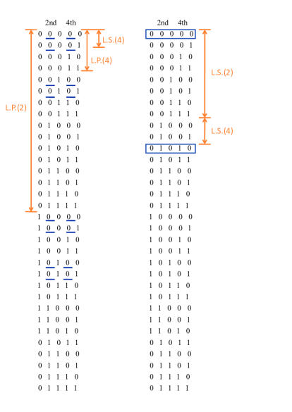
Figure 13: (Color online) The illustration of five spins basis.

References

- (1) A. Amico, R. Fazio, A. Osterloh, V. Vedral, Rev. Mod. Phys. 80, 518 (2008).
- (2) C.H. Bennett and D.P. DiVincenzo, Nature 404, 247 (2000).
- (3) C. Macchiavello, G.M. Palma and A. Zeilinger, Quantum Computation and Quantum Information Theory (World Scientific, 2000).
- (4) M. Nielsen and I. Chuang, Quantum Computation and Quantum Communication (Cambridge Univ. Press, Cambridge, 2000)
- (5) J. Gruska, Quantum Computing (McGraw-Hill, 1999)
- (6) V. Vedral, M.B. Plenio, M.A. Rippin and P.L. Knight, Phys. Rev. Lett. 78, 2275 (1997).
- (7) Y. Pashkin, T. Tilma, D. Averin, O. Astafiev, T. Yamamoto, Y. Nakamura, F. Nori, and J. Tsai, Int. J. Quantum Inf. 1, 421 (2003).
- (8) K. Maruyama, T. Iitaka, and F. Nori, Phys. Rev. A 75, 012325 (2007).
- (9) A. Osterloh, L. Amico, G. Falci, and R. Fazio, Nature 416, 608 (2002).
- (10) T. Osborne, and M. Nielsen, Phys. Rev. A 66, 032110 (2002).
- (11) A. Osterloh, L. Amico, F. Plastina, and R. Fazio, Proceedings of SPIE Quantum Information and Computation II, edited by E. Donkor, A. R. Pirich, and H. E. Brandt (SPIE, Bellingham, WA), 5436, 150 (2004).
- (12) G. Vidal, J. Latorre, E. Rico, and A. Kitaev, Phys. Rev. Lett. 90, 227902 (2003).
- (13) L.A. Wu, M.S. Sarandy and D.A. Lidar, Phys. Rev. Lett., 93, 250404-1 (2004).
- (14) L.A. Wu, M. S. Sarandy, D. A. Lidar, and L. J. Sham, Phys. Rev. A 74, 052335 (2006).
- (15) V. Akulin, G. Kurizki, and D.A. Lidar, J. Phys. B 40, E01 (2007).
- (16) D. A. Lidar, A. T. Rezakhani, and A. Hamma, J. Math. Phys. 50, 102106 (2009).
- (17) O. Osenda, Z. Huang and S. Kais, Phys. Rev. A 67, 062321-4 (2003).
- (18) Z. Huang, O. Osenda and S. Kais, Phys. Lett. A 322, 137 (2004).
- (19) Z. Huang and S. Kais, In. J. Quant. Information 3, 83 (2005).
- (20) Z. Huang and S. Kais, Phys, Rev. A 73, 022339 (2006).
- (21) S. Kais, Adv. Chem. Phys. 134, 493 (2007).
- (22) A. Sandvik and J. Kurkij, Phys. Rev. B 43, 5950 (191).
- (23) O. Syljuasen, and A.W. Sandvik, Phys. Rev. E 66, 046701 (2002).
- (24) O. Syluasen, Phys. Lett. A 322, 25 (2003).
- (25) O. Syluasen, Phy. Rev. A 68, 060301 (2003).
- (26) A. Sameh, and J.A. Wisniewski, SIAM J. Numerical Analysis, 19, 1243 (1982).
- (27) A. Sameh, and Z. Tong, J. of computational and applied mathematics 123, 155 (2000).
- (28) G. Sleijpen and H. van der Vorst, SIAM J. Matrix Anal. Appl. 17, 401 (1996).
- (29) W. Wooters, Phys. Rev. Lett. 80, 2245, (1998).
- (30) V. Coffman, J. Kundu, and W. K. Wootters, Phys. Rev. A 61, 052306 (2000).
- (31) T. J. Osborne, and F. Verstraete, Phys. Rev. Lett. 96, 220503 (2006).
- (32) C. Cohen-Tannoudji, B. Diu, and F. Laloe, Quantum Mechanics (Wiley-Interscience, 2006)
- (33) K. Penson, R. Jullien, and P. Pfeuty, Phys. Rev. Lett. B (19), 4653 (1979)
- (34) C. Hamer, J. Phys. A: Math. Gen. 33, 6683 (2000).
- (35) S. Kais and P. Serra Adv. Chem. Phys., 125, 1-100 (2003).
- (36) P. Serra, A.F. Stanton, and S. Kais, Phys. Rev. E 55, 1162 (1997).
- (37) S. Sachdev Quantum Phase Transitions (Cambridge Univ. Press, Cambridge, 2001).