Deterministic photon-photon $\sqrt{\rm SWAP}$ gate using a lambda system

Abstract

We theoretically present a method to realize a deterministic photon-photon $\sqrt{\rm SWAP}$ gate using a three-level lambda system interacting with single photons in reflection geometry. The lambda system is used completely passively as a temporary memory for a photonic qubit; the initial state of the lambda system may be arbitrary, and active control by auxiliary fields is unnecessary throughout the gate operations. These distinct merits make this entangling gate suitable for deterministic and scalable quantum computation.

Single photons are promising candidates for implementing qubits in quantum computation due to their long coherence times. Furthermore, one-qubit gates such as Hadamard and NOT gates can be readily realized using linear optical elements GK . Photonic qubits have the disadvantage that it is difficult to realize two-qubit controlled gates such as controlled-NOT gates due to the weak mutual interaction between photons Mil . This problem has been partially overcome by linear optics quantum computation, which enables probabilistic controlled gates that successfully operate depending on the measurement results of ancillary photons KLM ; OB .

In the quest for realizing deterministic controlled gates in quantum optics, a measurable nonlinear phase shift between single photons has been demonstrated using a cavity quantum electrodynamics system in the bad-cavity regime Tur . This system has the characteristic that radiation from the atom is nearly completely forwarded to a one-dimensional field that is determined by the radiation pattern of the cavity. Such one-dimensional configurations can be realized by a variety of physical systems, including a leaky resonator interacting with an atom or a quantum dot PB2 ; dot1 , a single emitter near a surface plasmon pla , and a superconducting qubit near a transmission line or a resonator cc1 ; Fan . Since the incident light inevitably interferes with the radiation from the system due to the reduced dimensionality, the effective light-matter interaction can be drastically enhanced under this configuration. Utilizing this property, several quantum devices have been proposed to date, such as controlled logic gates Duan1 ; Duan2 , quantum-state converters Cirac ; Sham ; Ima and entanglers of photonic or material qubits Ima ; Hu1 ; Hu2 . These devices perform their tasks with the help of active quantum control of the material part (such as initialization Duan1 ; Duan2 ; Cirac ; Sham ; Ima ; Hu1 ; Hu2 , single-qubit rotation Duan1 ; Duan2 , and classical pumping Cirac ; Sham ; Ima ) and by measurements Hu1 ; Hu2 .

In the present study, we theoretically point out a unique potential of a three-level lambda system coupled to a one-dimensional photon field in the reflection geometry. (A lambda system is hereafter referred to as an “atom”, although it can be implemented by other physical systems such as semiconductor quantum dots and superconducting Josephson junctions lam1 ; lam2 ; lam3 .) We show that a deterministic photon-photon $\sqrt{\rm SWAP}$ gate can be realized by using the atom completely passively as a temporary memory for photonic qubits; the initial state of the atom may be arbitrary including even mixed states, and active control of the atom is unnecessary throughout successive gate operations. These properties are quite advantageous when constructing scalable quantum networks. Furthermore, since the $\sqrt{\rm SWAP}$ gate constitutes a universal set of quantum gates together with one-qubit gates rtSWAP1 ; rtSWAP2 , the proposed scheme provides a vivid blueprint for future quantum computation, that is deterministic and scalable.

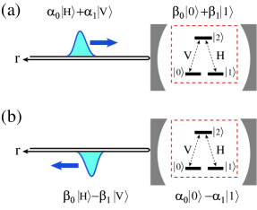
Figure 1: Interaction between a lambda system and a single photon propagating in one dimension. (a) Initial state. The photonic and atomic qubits may be in arbitrary states. (b) Final state. The lambda system is completely de-excited through radiative decay. The photonic and atomic qubits can be completely swapped under appropriate conditions.

The physical setup considered in this study is schematically illustrated in Fig. 1. The atom has two degenerate ground states ($|0\rangle$ and $|1\rangle$) and an excited state ($|2\rangle$), and the transition frequency is $\Omega$. The $|1\rangle\leftrightarrow|2\rangle$ and $|0\rangle\leftrightarrow|2\rangle$ transitions in the atom are assisted respectively by horizontally (H) and vertically (V) polarized photons and the radiative decay rates for the $|2\rangle\to|1\rangle$ and $|2\rangle\to|0\rangle$ transitions are $\Gamma_{H}$ and $\Gamma_{V}$. The total Hamiltonian including the atom and the photon field is given, under the rotating-wave approximation, by (putting $\hbar=c=1$)

$${\cal H} = \Omega\sigma_{22}+\int dk\left[kh_{k}^{\dagger}h_{k}+i\sqrt{\frac{\Gamma_{H}}{2\pi}}(\sigma_{21}h_{k}-h_{k}^{\dagger}\sigma_{12})\right]$$ (1)

$$+\int dk\left[kv_{k}^{\dagger}v_{k}+i\sqrt{\frac{\Gamma_{V}}{2\pi}}(\sigma_{20}v_{k}-v_{k}^{\dagger}\sigma_{02})\right],$$

where $\sigma_{ij}(=|i\rangle\langle j|)$ is the atomic transition operator, and $h_{k}$ ($v_{k}$) is the annihilation operator for the H (V) polarized photon with wave number $k$. As shown in Fig. 1, we define the spatial coordinate $r$ along the propagation direction of the photon, and assign the negative (positive) region to the input (output) ports. The real-space representation of the field operator $\widetilde{h}_{r}$ is defined as the Fourier transform of $h_{k}$ by $\widetilde{h}_{r}=(2\pi)^{-1/2}\int dke^{ikr}h_{k}$.

The initial states of the photon and the atom are given by $\alpha_{0}|H\rangle+\alpha_{1}|V\rangle$ and $\beta_{0}|0\rangle+\beta_{1}|1\rangle$, respectively [Fig. 1(a)]. We denote the wave packet of the input photon in the real-space representation by $f(r)$, which is normalized as $\int dr|f(r)|^{2}=1$. The four basis states of the input are then given, in the multimode notation, by

$$|H,0\rangle = \int drf(r)\widetilde{h}_{r}^{\dagger}|0\rangle,$$ (2)

$$|H,1\rangle = \int drf(r)\widetilde{h}_{r}^{\dagger}|1\rangle,$$ (3)

$$|V,0\rangle = \int drf(r)\widetilde{v}_{r}^{\dagger}|0\rangle,$$ (4)

$$|V,1\rangle = \int drf(r)\widetilde{v}_{r}^{\dagger}|1\rangle.$$ (5)

The output states are determined by the Schrödinger equations, $|H,0\rangle\to e^{-i{\cal H}t}|H,0\rangle$ etc, where ${\cal H}$ is the Hamiltonian of Eq. (1) and the final time $t$ is a sufficiently large time at which the atom is completely de-excited [Fig. 1(b)]. The time evolutions of $|H,0\rangle$ and $|V,1\rangle$ are trivial, since the input photon does not interact with the atom and therefore propagates freely. In contrast, the time evolutions of $|H,1\rangle$ and $|V,0\rangle$ are nontrivial, since the input photon may interact with the atom in these cases. The output state vectors are given by

$$|H,0\rangle \to \int drg_{1}(r,t)\widetilde{h}_{r}^{\dagger}|0\rangle,$$ (6)

$$|H,1\rangle \to \int drg_{3}(r,t)\widetilde{h}_{r}^{\dagger}|1\rangle-\int drg_{2}(r,t)\widetilde{v}_{r}^{\dagger}|0\rangle,$$ (7)

$$|V,0\rangle \to \int drg_{4}(r,t)\widetilde{v}_{r}^{\dagger}|0\rangle-\int drg_{2}(r,t)\widetilde{h}_{r}^{\dagger}|1\rangle,$$ (8)

$$|V,1\rangle \to \int drg_{1}(r,t)\widetilde{v}_{r}^{\dagger}|1\rangle,$$ (9)

where $g_{1}$, $g_{2}$, $g_{3}$ and $g_{4}$ are determined by

$$g_{1}(r,t) = f(r-t),$$ (10)

$$g_{2}(r,t) = \sqrt{\Gamma_{H}\Gamma_{V}}s(t-r),$$ (11)

$$g_{3}(r,t) = f(r-t)-\Gamma_{H}s(t-r),$$ (12)

$$g_{4}(r,t) = f(r-t)-\Gamma_{V}s(t-r),$$ (13)

where $s(t)$ is the atomic coherence induced by the input photon, which evolves as

$$\frac{d}{dt}s(t)=\left(-i\Omega-\frac{\Gamma_{H}+\Gamma_{V}}{2}\right)s(t)+f(-t).$$ (14)

These equations are derived in Appendix A The probabilities of the occurrence and absence of the $|H,1\rangle\leftrightarrow|V,0\rangle$ transition are quantified by $P=\int dr|g_{2}(r,t)|^{2}$ and $P^{\prime}=\int dr|g_{3}(r,t)|^{2}$=$\int dr|g_{4}(r,t)|^{2}$, which satisfy the sum rule of $P+P^{\prime}=1$.

We here consider a case in which the pulse length $l$ of the input photon is sufficiently long to satisfy $l\gg\Gamma_{H,V}^{-1}$. In this case, Eq. (14) can be solved adiabatically. Denoting the detuning of the input photon by $\omega$ [namely, $f(r)\sim e^{i(\Omega+\omega)r}$], $s(t)$ is given by $s(t)=\frac{2}{\Gamma_{H}+\Gamma_{V}-2i\omega}f(-t)$. Substituting this into Eqs. (6)–(13) and neglecting the translational motion of the photon, the four basis states are transformed as follows on reflection:

$$|H,0\rangle \to |H,0\rangle,$$ (15)

$$|H,1\rangle \to {\textstyle\frac{\Gamma_{V}-\Gamma_{H}-2i\omega}{\Gamma_{H}+\Gamma_{V}-2i\omega}|H,1\rangle-\frac{2\sqrt{\Gamma_{H}\Gamma_{V}}}{\Gamma_{H}+\Gamma_{V}-2i\omega}|V,0\rangle,}$$ (16)

$$|V,0\rangle \to {\textstyle-\frac{2\sqrt{\Gamma_{H}\Gamma_{V}}}{\Gamma_{H}+\Gamma_{V}-2i\omega}|H,1\rangle+\frac{\Gamma_{H}-\Gamma_{V}-2i\omega}{\Gamma_{H}+\Gamma_{V}-2i\omega}|V,0\rangle,}$$ (17)

$$|V,1\rangle \to |V,1\rangle.$$ (18)

The case of $\Gamma_{H}=\Gamma_{V}$ is of particular interest as a quantum logic gate. When the input photon is in resonance with the atom ($\omega=0$), this gate behaves as an atom-photon SWAP gate. As illustrated in Fig. 1, the quantum states of atomic and photonic qubits are exchanged on reflection as

$$(\alpha_{0}|H\rangle+\alpha_{1}|V\rangle)(\beta_{0}|0\rangle+\beta_{1}|1\rangle)\to(\beta_{0}|H\rangle-\beta_{1}|V\rangle)(\alpha_{0}|0\rangle-\alpha_{1}|1\rangle).$$ (19)

Thus, the atom functions as a quantum memory of the photonic qubit, which is indispensable for long-distance quantum key distribution using quantum repeaters. On the other hand, when the detuning of the input photon is set to the linewidth of the atom ($\omega=\pm\Gamma_{H}$), this gate behaves as an atom-photon $\sqrt{\rm SWAP}$ gate. For example, when $\omega=-\Gamma_{H}$, $|H,1\rangle\to 2^{-1/2}(e^{i\pi/4}|H,1\rangle+e^{3i\pi/4}|V,0\rangle)$ and $|V,0\rangle\to 2^{-1/2}(e^{3i\pi/4}|H,1\rangle+e^{i\pi/4}|V,0\rangle)$, whereas $|H,0\rangle$ and $|V,1\rangle$ remain unchanged.

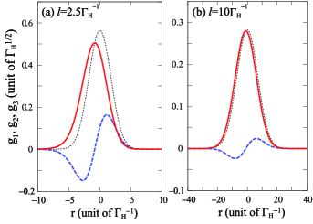
Figure 2: Shapes of the output wave packets, $g_{1}$ (thin dotted line), $g_{2}$ (solid line) and $g_{3}$ (dashed line), for the case of the atom-photon SWAP gate ($\Gamma_{H}=\Gamma_{V}$ and $\omega=0$). The natural phase factor $e^{i\Omega(r-t)}$ is removed. The pulse length is (a) $l=2.5\Gamma_{H}^{-1}$ and (b) $l=10\Gamma_{H}^{-1}$.

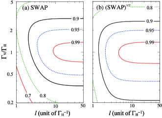
Figure 3: Contour plots of the average gate fidelities for the atom-photon (a) SWAP ($\omega=0$) and (b) $\sqrt{\rm SWAP}$ ($\omega=-\Gamma_{H}$) gates, as functions of the pulse length $l$ and $\Gamma_{V}/\Gamma_{H}$.

To observe the effects of a finite pulse length $l$, the shapes of $g_{1}$, $g_{2}$ and $g_{3}$(=$g_{4}$) are plotted in Fig. 2 for the case of the atom-photon SWAP gate ($\Gamma_{H}=\Gamma_{V}$ and $\omega=0$). The input mode function is assumed to be Gaussian, $f(r)=(2/\pi l^{2})^{1/4}\exp(-r^{2}/l^{2}+i\Omega r)$. It is observed that $g_{2}$ is slightly delayed relative to $g_{1}$ due to absorption and re-emission by the atom. The delay time is of the order of $\Gamma_{H}^{-1}$. However, this delay becomes negligible when the input pulse is long ($l\gg\Gamma_{H}^{-1}$) as in Fig. 2(b). $g_{2}$ becomes almost identical to $g_{1}$ whereas $g_{3}$ vanishes. The average gate fidelities of the atom-photon SWAP and $\sqrt{\rm SWAP}$ gates are respectively given by avgf1 ; avgf2

$$\bar{F}_{\rm SWAP} = \frac{1+\left|1+\int drg_{2}^{\ast}g_{1}\right|^{2}}{5},$$ (20)

$$\bar{F}_{\sqrt{\rm SWAP}} = \frac{1+\left|1+\frac{1+i}{4}\int dr(g_{3}^{\ast}+g_{4}^{\ast}-2ig_{2}^{\ast})g_{1}\right|^{2}}{5}.$$ (21)

In Fig. 3, $\bar{F}_{\rm SWAP}$ and $\bar{F}_{\sqrt{\rm SWAP}}$ are plotted as functions of the pulse length $l$ and the ratio $\Gamma_{V}/\Gamma_{H}$ of the atomic decay rates. The conditions for achieving high-fidelity operations are given by $l\gg\Gamma_{H,V}^{-1}$ and $\Gamma_{H}/\Gamma_{V}\simeq 1$ for both gates.

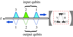
Figure 4: Illustration of the photon-photon $\sqrt{\rm SWAP}$ gate. Photons 1 and 3 are in resonance with the atom ($\omega=0$), whereas photon 2 is detuned ($\omega=\pm\Gamma_{H}$). The input qubits are the polarization states of photons 1 and 2, whereas the output qubits are those of photons 3 and 2.

These atom–photon gates are highly useful for a variety of purposes in quantum information processing. As an illuminative example, we show that a photon-photon $\sqrt{\rm SWAP}$ gate that operates deterministically and with a high gate fidelity can be realized by using an atom as a temporary quantum memory. This fact implies that deterministic all-optical quantum computation is possible, since a $\sqrt{\rm SWAP}$ gate constitutes a universal set of quantum gates together with one-photon gates, which can be realized by linear optical elements. Figure 4 shows a schematic illustration of the photon-photon $\sqrt{\rm SWAP}$ gate. Three photons (1, 2, and 3) are forwarded to the atom with sufficiently large time intervals between them. The initial state of the atom may be an arbitrary superposition of the two ground states, $|0\rangle$ and $|1\rangle$. Photons 1 and 3 are in resonance with the atom ($\omega=0$), whereas photon 2 is slightly detuned ($\omega=\pm\Gamma_{H}$). We assign photons 1 and 2 as the input qubits, and photons 3 and 2 as the output qubits. We can then confirm the following $\sqrt{\rm SWAP}$ operation (for example, for $\omega=-\Gamma_{H}$ for photon 2):

$$|H\rangle_{1}|H\rangle_{2} \to |H\rangle_{3}|H\rangle_{2},$$ (22)

$$|H\rangle_{1}|V\rangle_{2} \to 2^{-1/2}(e^{i\pi/4}|H\rangle_{3}|V\rangle_{2}+e^{-i\pi/4}|V\rangle_{3}|H\rangle_{2})$$ (23)

$$|V\rangle_{1}|H\rangle_{2} \to 2^{-1/2}(e^{-i\pi/4}|H\rangle_{3}|V\rangle_{2}+e^{i\pi/4}|V\rangle_{3}|H\rangle_{2})$$ (24)

$$|V\rangle_{1}|V\rangle_{2} \to |V\rangle_{3}|V\rangle_{2}.$$ (25)

The initial states of the atom and photon 3, both of which may be arbitrary, are respectively transferred to the final states of photon 1 and the atom in the following manner:

$$\alpha_{0}|0\rangle_{a}+\alpha_{1}|1\rangle_{a} \to \alpha_{0}|H\rangle_{1}-\alpha_{1}|V\rangle_{1},$$ (26)

$$\beta_{0}|H\rangle_{3}+\beta_{1}|V\rangle_{3} \to \beta_{0}|0\rangle_{a}-\beta_{1}|1\rangle_{a},$$ (27)

where the subscript “$a$” denotes the atom. These states are unentangled with the output qubits and therefore do not affect the gate. They can also be recycled for subsequent gate operations. Four comments on this gate are in order. (i) This gate enables the $\sqrt{\rm SWAP}$ operation between two photons having different frequencies. The SWAP operation between them can be achieved by using this gate twice. Therefore, the current scheme can be extended to construct the $\sqrt{\rm SWAP}$ operation between two photons having the same frequency. (ii) The present scheme does not depend on optical nonlinearity nor interference between single photons. Therefore, the proposed gate operates with a high fidelity irrespective of the pulse shapes and time intervals of the input photons, provided the pulses are sufficiently long. This implies that high stability of optical paths, which is essential in many optical experiments, is not required. (iii) The atom may be in an arbitrary de-excited state initially. Even if the atom is in a mixed state, it can be restored to a pure state automatically by the first input photon. Therefore, the quantum coherence of the atom should be maintained only during the three photons interact with the atom. (iv) Throughout successive gate operations, there is no need for auxiliary control fields to manipulate the atomic quantum state. Namely, the atom is used completely passively as a temporary quantum memory. These merits make the proposed scheme quite advantageous for constructing a scalable quantum network.

Finally, we estimate the effects of practical noises and imperfections such as radiative loss, finite spin-coherence times, discrepancy between $\Gamma_{H}$ and $\Gamma_{V}$, and finite pulse lengths, assuming that the lambda system is implemented by a charged quantum dot in a photonic crystal nanocavity. The typical values of the cavity-QED parameters are $(g,\gamma,\kappa)\sim 2\pi\times(16,0.2,32)$ GHz, and therefore $\Gamma(\sim g^{2}/\kappa)\sim 2\pi\times 8$ GHz. Then, the photon loss rate is estimated at $\gamma/(\Gamma+\gamma)\sim$2.5% per one gate operation. The gate fidelity can be estimated with a help of Fig. 3; when the pulse length $l$ is 400 ps (20$\Gamma^{-1}$) and $\Gamma_{H}/\Gamma_{V}=1.4$ for example, the fidelity of the photon-photon $\sqrt{\rm SWAP}$ gate becomes $(0.99)^{3}\sim 0.97$. The time intervals between photons should be shorter than the homogeneous spin-coherence time of the order of $\mu$s spin1 ; spin2 .

In summary, we have investigated the interaction between a three-level lambda system and a single photon propagating in one dimension (Fig. 1), and observed that this atom–photon system behaves as SWAP and $\sqrt{\rm SWAP}$ gates when the two decay rates in the atom are close ($\Gamma_{H}\simeq\Gamma_{V}$). Furthermore, successive input of three photons enables a photon-photon $\sqrt{\rm SWAP}$ gate (Fig. 4) that can operate deterministically. The distinct advantage of the proposed gate is that the atomic qubit is used completely passively; the atomic qubit may be in an arbitrary initial state, and any active control of the atomic qubit is unnecessary throughout the gate operations. Therefore, the proposed gate is suitable for constructing scalable quantum networks and computers.

The authors are grateful to T. Yamamoto, T. Kato, R. Shimizu, and N. Matsuda for fruitful discussions. This research was partially supported by the Nakajima Foundation, MEXT KAKENHI (17GS1204, 21104507), the Special Coordination Funds for Promoting Science and Technology, and the CREST program of the Japan Science and Technology Agency (JST).

Appendix A Derivation of Eqs. (10)–(14)

A.1 Heisenberg equations

From the Hamiltonian of Eq. (1), the Heisenberg equations for $h_{k}$ and $\sigma_{12}$ are given by

$$\frac{d}{d\tau}h_{k} = -ikh_{k}-\sqrt{\frac{\Gamma_{H}}{2\pi}}\sigma_{12},$$ (28)

$$\frac{d}{d\tau}\sigma_{12} = -i\Omega\sigma_{12}+\sqrt{\Gamma_{H}}(\sigma_{11}-\sigma_{22})\widetilde{h}_{0}+\sqrt{\Gamma_{V}}\sigma_{10}\widetilde{v}_{0},$$ (29)

where $\widetilde{h}_{0}$ is the real-space representation of the field operator at $r=0$, namely, $\widetilde{h}_{0}=(2\pi)^{-1/2}\int dkh_{k}$. The initial and final moments are respectively set at $\tau=0$ and $t$. Then, from Eq. (28), $h_{k}(\tau)$ ($0<\tau<t$) is represented in two ways,

$$h_{k}(\tau) = h_{k}(0)e^{-ik\tau}-\sqrt{\frac{\Gamma_{H}}{2\pi}}\int_{0}^{\tau}d\tau^{\prime}\sigma_{12}(\tau^{\prime})e^{-ik(\tau-\tau^{\prime})},$$ (30)

$$h_{k}(\tau) = h_{k}(t)e^{-ik(\tau-t)}+\sqrt{\frac{\Gamma_{H}}{2\pi}}\int_{\tau}^{t}d\tau^{\prime}\sigma_{12}(\tau^{\prime})e^{-ik(\tau-\tau^{\prime})}.$$ (31)

As the Fourier transform of the above equations, $\widetilde{h}_{0}(\tau)$ is given by

$$\widetilde{h}_{0}(\tau) = \widetilde{h}_{-\tau}(0)-\frac{\sqrt{\Gamma_{H}}}{2}\sigma_{12}(\tau),$$ (32)

$$\widetilde{h}_{0}(\tau) = \widetilde{h}_{t-\tau}(t)+\frac{\sqrt{\Gamma_{H}}}{2}\sigma_{12}(\tau).$$ (33)

Equating the right-hand sides, introducing a new label $r(=t-\tau)$, and using the symmetry of the system, we obtain the following set of equations:

$$\widetilde{h}_{r}(t) = \widetilde{h}_{r-t}(0)-\sqrt{\Gamma_{H}}\sigma_{12}(t-r),$$ (34)

$$\widetilde{v}_{r}(t) = \widetilde{v}_{r-t}(0)-\sqrt{\Gamma_{V}}\sigma_{02}(t-r),$$ (35)

where $0<r<t$. These equations are known as the input-output relation. Substituting Eq. (32) into Eq. (29) and using the symmetry, we obtain

$$\frac{d}{d\tau}\sigma_{12} = \left(-i\Omega-\frac{\Gamma_{H}+\Gamma_{V}}{2}\right)\sigma_{12}+\sqrt{\Gamma_{H}}(\sigma_{11}-\sigma_{22})\widetilde{h}_{-\tau}(0)+\sqrt{\Gamma_{V}}\sigma_{10}\widetilde{v}_{-\tau}(0),$$ (36)

$$\frac{d}{d\tau}\sigma_{02} = \left(-i\Omega-\frac{\Gamma_{H}+\Gamma_{V}}{2}\right)\sigma_{02}+\sqrt{\Gamma_{V}}(\sigma_{00}-\sigma_{22})\widetilde{v}_{-\tau}(0)+\sqrt{\Gamma_{H}}\sigma_{01}\widetilde{h}_{-\tau}(0).$$ (37)

A.2 Temporal evolution of $|V,0\rangle$

We investigate the temporal evolution of the input states, Eqs. (2)–(5). As a nontrivial case, we consider here the evolution of $|V,0\rangle$. From Eqs. (4) and (8), the input and output state vectors are written as

$$|\varphi_{in}\rangle = \int drf(r)\widetilde{v}_{r}^{\dagger}|0\rangle,$$ (38)

$$|\varphi_{out}\rangle = \int drg_{4}(r;t)\widetilde{v}_{r}^{\dagger}|0\rangle-\int drg_{2}(r;t)\widetilde{h}_{r}^{\dagger}|1\rangle.$$ (39)

These two state vectors are related by $|\varphi_{out}\rangle=e^{-i{\cal H}t}|\varphi_{in}\rangle$. The following two properties are useful in the arguments below: (I) $e^{-i{\cal H}t}|0\rangle=|0\rangle$ and $e^{-i{\cal H}t}|1\rangle=|1\rangle$ since ${\cal H}|0\rangle={\cal H}|1\rangle=0$. (II) $\widetilde{h}_{r}(0)|\varphi_{in}\rangle=0$ and $\widetilde{v}_{r}(0)|\varphi_{in}\rangle=f(r)|0\rangle$, since the field commutators are given by $[\widetilde{v}_{r},\widetilde{v}_{r^{\prime}}^{\dagger}]=\delta(r-r^{\prime})$ and $[\widetilde{h}_{r},\widetilde{v}_{r^{\prime}}^{\dagger}]=0$.

From Eq. (39) and the property (I), $g_{2}$ and $g_{4}$ are determined by

$$g_{2}(r,t) = -\langle 1|\widetilde{h}_{r}|\varphi_{out}\rangle=-\langle 1|\widetilde{h}_{r}(t)|\varphi_{in}\rangle,$$ (40)

$$g_{4}(r,t) = \langle 0|\widetilde{v}_{r}|\varphi_{out}\rangle=\langle 0|\widetilde{v}_{r}(t)|\varphi_{in}\rangle,$$ (41)

where $A(t)=e^{i{\cal H}t}Ae^{-i{\cal H}t}$ (Heisenberg representation). Using Eqs. (34), (35), (38) and the property (II), $g_{2}$ and $g_{4}$ are recast into the following forms:

$$g_{2}(r,t) = \sqrt{\Gamma_{H}}\langle 1|\sigma_{12}(t-r)|\varphi_{in}\rangle,$$ (42)

$$g_{4}(r,t) = f(r-t)-\sqrt{\Gamma_{V}}\langle 0|\sigma_{02}(t-r)|\varphi_{in}\rangle.$$ (43)

$s_{02}(\tau)\equiv\langle 0|\sigma_{02}(\tau)|\varphi_{in}\rangle$ and $s_{12}(\tau)\equiv\langle 1|\sigma_{12}(\tau)|\varphi_{in}\rangle$ represent the atomic coherence induced by the input photon. Their equations of motion are given, from Eqs. (36)–(38) and the property (II), by

$$\frac{d}{d\tau}s_{02}(\tau) = \left(-i\Omega-\frac{\Gamma_{H}+\Gamma_{V}}{2}\right)s_{02}(\tau)+\sqrt{\Gamma_{V}}\langle 0|\sigma_{00}(\tau)-\sigma_{22}(\tau)|0\rangle f(-\tau),$$ (44)

$$\frac{d}{d\tau}s_{12}(\tau) = \left(-i\Omega-\frac{\Gamma_{H}+\Gamma_{V}}{2}\right)s_{12}(\tau)+\sqrt{\Gamma_{V}}\langle 1|\sigma_{10}(\tau)|0\rangle f(-\tau).$$ (45)

Since $\langle 0|\sigma_{00}(\tau)-\sigma_{22}(\tau)|0\rangle=\langle 1|\sigma_{10}(\tau)|0\rangle=1$ from the property (I), $s_{02}(\tau)$ and $s_{12}(\tau)$ becomes identical. Introducing $s=s_{02}/\sqrt{\Gamma_{V}}=s_{12}/\sqrt{\Gamma_{V}}$, we obtain

$$g_{2}(r,t) = \sqrt{\Gamma_{H}\Gamma_{V}}s(t-r),$$ (46)

$$g_{4}(r,t) = f(r-t)-\Gamma_{V}s(t-r),$$ (47)

$$\frac{d}{d\tau}s(\tau) = \left(-i\Omega-\frac{\Gamma_{H}+\Gamma_{V}}{2}\right)s(\tau)+f(-\tau).$$ (48)

Thus, Eqs. (11), (13) and (14) of the main text are derived.

References

(1)
C. C. Gerry and P. L. Knight,
Introductory Quantum Optics
(Cambridge University Press, Cambridge, England, 2005),
Sec. 11.11.
(2)
G. J. Milburn, Phys. Rev. Lett. 62, 2124 (1989).
(3)
E. Knill, R. Laflamme and G. J. Milburn, Nature 409, 46 (2001).
(4)
J. L. O’Brien, Science 318, 1567 (2007).
(5)
Q. A. Turchette, C. J. Hood, W. Lange, H. Mabuchi and H. J. Kimble,
Phys. Rev. Lett. 75, 4710 (1995).
(6)
T. Aoki et al.,
Phys. Rev. Lett. 102, 083601 (2009).
(7)
I. Fushman et al., Science 320, 769 (2008).
(8)
D. E. Chang, A. S. Sørensen, E. A. Demler, and M. D. Lukin,
Nature Phys. 3, 807 (2007).
(9)
A. Blais et al., Phys. Rev. A 69, 062320 (2004).
(10)
J. T. Shen and S. Fan,
Phys. Rev. Lett. 95, 213001 (2005).
(11)
L. -M. Duan and H. J. Kimble,
Phys. Rev. Lett. 92, 127902 (2004).
(12)
B. Wang and L. -M. Duan,
Phys. Rev. A 75, 050304(R) (2007).
(13)
J. I. Cirac, P. Zoller, H. J. Kimble, and H. Mabuchi,
Phys. Rev. Lett. 78, 3221 (1997).
(14)
W. Yao, R. -B. Liu, and L. J. Sham,
Phys. Rev. Lett. 95, 030504 (2005).
(15)
D. Pinotsi and A. Imamoglu,
Phys. Rev. Lett. 100, 093603 (2008).
(16)
C. Y. Hu et al.,
Phys. Rev. B 78, 085307 (2008).
(17)
C. Y. Hu, W. J. Munro and J. G. Rarity,
Phys. Rev. B 78, 125318 (2008).
(18)
X. Xu et al.,
Nature Phys. 4, 692 (2008).
(19)
D. Press, T. D. Ladd, B. Zhang, and Y. Yamamoto,
Nature 456, 218 (2008).
(20)
J. Q. You and F. Nori,
Phys. Today 58 (11), 42 (2005).
(21)
D. Loss and D. P. DiVincenzo,
Phys. Rev. A 57, 120 (1998).
(22)
K. Eckert et al.,
Phys. Rev. A 66, 042317 (2002).
(23)
See EPAPS Document No. [number will be inserted by publisher]
for derivation of the output wave packets.
For more information on EPAPS,
see http://www.aip.org/pubservs/epaps.html.
(24)
M. Horodecki, P. Horodecki and R. Horodecki,
Phys. Rev. A 60, 1888 (1999).
(25)
M. A. Nielsen,
Phys. Lett. A 303, 249 (2002).