Convergence conditions for iterative methods seeking multi-component solitary waves with prescribed quadratic conserved quantities
Abstract
We obtain local (i.e., linearized) convergence conditions for iterative methods that seek solitary waves with prescribed values of quadratic conserved quantities of multi-component Hamiltonian nonlinear wave equations. These conditions extend the ones found for single-component solitary waves in [J. Yang and T.I. Lakoba, Stud. Appl. Math. 120, 265–292 (2008)]. We also show that, and why, these convergence conditions coincide with dynamical stability conditions for ground-state solitary waves.
Keywords: Coupled nonlinear wave equations, Solitary waves, Iterative methods.
PACS: 03.75.Lm, 05.45.Yv, 42.65.Tg, 47.35.Fg.
Solitary wave solutions of most nonlinear wave equations can be found only numerically. Recently, J. Yang and the present author obtained [1] conditions under which an iterative numerical method can converge to stationary solitary waves of single-component Hamiltonian nonlinear wave equations. When this method, in what follows referred to as the imaginary-time evolution method (ITEM), converges, it provides one with a numerical approximation of a solitary waves with a prescribed value of a quadratic conserved quantity usually referred to either as power or the number of particles. However, many phenomena are described not by a single equation but by systems of coupled equations. Therefore, it is of interest to obtain conditions under which a multi-component counterpart of the ITEM would be guaranteed to converge to, i.e., find, a multi-component solitary wave. We obtain such a condition in this work. Moreover, generalizing an observation made in [1], we show that the multi-component ITEM converges only to those ground states of nonlinear wave equations which are dynamically stable, and explain why this is the case.
1 Introduction and background
For the single-equation case considered in Ref. [1], the power of a solitary wave is
| (1.1) |
where is the real-valued field of the solitary wave and is the spatial coordinate. (Here and below, if the limits of the integration are not indicated, the integration is assumed to be over the entire spatial domain.) For example, if the time-dependent wave satisfies a Nonlinear Schrödinger-type (NLS-type) equation
| (1.2) |
where is the Laplacian, then upon the substitution , where is real, Eq. (1.2) reduces to
| (1.3a) | |||
| where | |||
| (1.3b) | |||
The parameter is referred to as the propagation constant of the solitary wave. A straightforward calculation shows that the power is conserved by the evolution equation (1.2). Thus, can be parametrized either by or by , so that one can write .
The method analyzed in [1] finds the solution with a prescribed value of by iterations:
| (1.4a) | |||
| (1.4b) | |||
| (1.4c) |
where is an auxiliary parameter, and a positive definite operator can be conveniently chosen in the form mimicking the linear constant-coefficient part of in (1.3a):
| (1.5) |
The purposes of and in (1.4b) will be clarified shortly. The inner product is defined as
| (1.6) |
Methods similar to (1.4c) had also been considered for finding solitary waves in the past (see, e.g., [2]–[5]). However, it was in [1] where the convergence conditions of the specific version, (1.4c), of the ITEM were found in terms of the properties of the linearized operator of Eq. (1.3a). Namely, Eqs. (1.4c) are linearized by a substitution
| (1.7) |
which results in [1]
| (1.8) |
Here is the linearized operator of in Eq. (1.3a). For example, for given by (1.3b),
| (1.9) |
The ITEM (1.4c) converges if the eigenvalues of the right-hand side of its linearization (1.8) are located between and . The first of these conditions implies that
| (1.10) |
where is the most negative eigenvalue of . (In practice, the maximum can be easily found by just a few trials, and then the value leading to an optimal convergence rate is usually somewhat smaller than ; see Fig. 3 and Eq. (47) in [1].) The second condition can be shown [1] to be related to the properties of the original equation (1.3a) and its linearized operator as follows [6]. First, let us denote
| (1.11) |
(and similarly for any other operator or matrix). Next, assume that we are considering the generic case whereby the null space of does not contain any functions other than those of the modes which are associated with translational invariance of the solitary wave along . Then, under condition (1.10), the ITEM (1.4c) converges provided that either
| (1.12a) | |||
| or | |||
| (1.12b) | |||
In all the other cases algorithm (1.4c) diverges [9]. Remarkably, as pointed out in [1], these convergence conditions are the same as the stability conditions of nodeless solitary waves in the NLS-type evolution equation (1.2) [8]. In other words, the ITEM (1.4c) converges only to those nodeless solitary waves of (1.2) that are dynamically linearly stable. (Let us note, in passing, that iterative methods that are guaranteed to converge to any solitary wave, stable or unstable, were first proposed in [3] and later developed in [10].)
The purpose of using operator in (1.4b) is to considerably reduce the magnitude of the most negative eigenvalue of operator compared to that of [3, 1, 10]. This is analogous to preconditioning a poorly conditioned matrix when solving a linear equation by an iterative method; this can considerably improve the convergence rate of the iterations (see, e.g., [7], Lecture 40). In regards to implementing , note that it is a differential operator with constant coefficients and hence has a simple representation in the Fourier space. Therefore, and are easily computed using the direct and inverse Fast Fourier Transforms, which are available as built-in commands in all major computing software.
Note that the propagation constant in the ITEM (1.4c) is not prescribed but computed iteratively. Numerical methods for finding solutions of Eq. (1.3b) with a specified value of rather than with a specified value of power (1.1) have also been considered in quite a few studies (see, e.g., references in [11]), and we will not consider them in this work.
In this paper, we derive convergence conditions of a generalization of the ITEM (1.4c) for multi-component solitary waves. Such a generalization was proposed in [11] (but see also Section 4.3 in [10]), and its algorithm is presented in Section 2. Note that in [11], we also proposed another method that finds solitary waves with the same conserved quantities as the ITEM but converges faster; moreover, it converges much faster than the ITEM when the latter converges slowly. This method is a modified form of the well-known Conjugate Gradient method (CGM; see, e.g., [7], Lecture 38), and its algorithm is given in Appendix for the reader’s convenience. In [11] we showed that this modified CGM has the same convergence conditions as the ITEM. Therefore, these convergence conditions, which generalize conditions (1.12b), apply to both the ITEM and modified CGM. The derivation of these conditions is the main result of this paper and is presented in Section 3. This derivation is based on the idea of Ref. [12], where it was used to establish stability conditions for a certain class of multi-component solitary waves. In fact, our convergence conditions of the ITEM and modified CGM turn out to be the same as the stability conditions derived in [12]. This relation between the two sets of conditions generalizes a similar fact pointed out in [1] for single-component equations, and in Section 5 we explain under what circumstances such a coincidence of the convergence and stability conditions occurs. In Section 4 we provide a geometrical argument that facilitates intuitive interpretation of the convergence conditions derived in Section 3 for the special case where the solitary wave has two quadratic conserved quantities. In Section 6 we summarize the results of this work. Let us emphasize that numerical examples involving the multi-component ITEM and CGM are not a subject of this analytical study; the interested reader can find such examples in Ref. [11].
2 ITEM algorithm for multi-component solitary waves
Let us begin with an example that will motivate introduction of some new notations. The following system describes pulse evolution in a two-core nonlinear directional fiber coupler where each core supports two orthogonal polarizations of light [13]:
| (2.1) |
Here and are the pairs of orthogonal polarizations in the two cores. The quadratic quantities conserved by these equations and generalizing (1.1) are:
| (2.2) |
where . Upon the substitution
| (2.3) |
where can (for the purpose of this example) be chosen to be real-valued, system (2.1) reduces to:
| (2.4) |
where . Then the powers of the individual components are
| (2.5) |
We now generalize this example to an -component system possessing an -component vector of conserved quantities , so that the th component of is:
| (2.6) |
where the solitary wave is . As illustrated in the above example with and , the number of conserved quantities can be less than the number of the components of the solitary wave: . Other examples where the situation takes place include: a system of NLS-type equations coupled coherently via phase-sensitive nonlinear terms (as opposed to linear ones as in (2.1)); the well-known system of three waves interacting via quadratic nonlinearity [14, 15]; and any system of coupled carrier-wave (also known as long-wave, or Korteweg–de Vries-type (KdV-type)) equations, as we will explain at the end of Section 5. To emphasize the possibility of having , we use a different vector notation for than for . Now, the matrix in (2.6) is assumed to be in reduced echelon form (see any textbook on undergraduate Linear Algebra) and, in addition, its columns are arranged so that
| (2.7) |
In (2.2), matrix is the matrix.
The multi-component generalization of Eqs. (1.3a) and (1.4a) is
| (2.8a) | |||
| (2.8b) |
For example, in (2.4), is the first term (the vector), and is the first factor of the second term (the matrix) on the left-hand side. The matrix is a self-adjoint positive definite operator. For optimal preconditioning, its differential part should mimic the highest derivative in the linear part of . For example, for the in (2.4), can be chosen as a diagonal matrix with its diagonal entries of the form (1.5).
The multi-component version of the ITEM (1.4c) is:
| (2.9a) | |||
| (2.9b) |
where
Note that, by (2.7), the numerator of the fraction under the square root equals . Let us emphasize that if , then (2.9b) specifies only that the components of have their prescribed values but does not impose any other conditions on the powers, , of the individual components of the solitary wave.
As we noted in Section 1, in [11] we proposed a modified CGM that converges under the same conditions that we will establish for the ITEM (2.9b), but faster. Moreover, it converges much faster when the ITEM converges slowly. Its algorithm, however, is somewhat less transparent than (2.9b), and therefore we state it in Appendix. Let us reiterate: The convergence analysis that we will present in Section 3 applies both to the ITEM and the modified CGM. We advocate using the latter method when the slow convergence of the ITEM justifies spending a little extra effort on programming the algorithm of the CGM.
As in the single-component case, we perform convergence analysis of the ITEM (2.9b) using linearization analogous to (1.7). A tedious but straightforward calculation shows that the linearized operator of the right-hand side of Eq. (2.9a) is:
| (2.10) |
Here is the linearized operator of in (2.8a) obtained when the last term in that equation is replaced by ; compare with (2.4). (Although is not prescribed but instead is iteratively computed within the method, its exact value can still be used in the convergence analysis.) For Hamiltonian wave equations, is self-adjoint. Next, the conservation of implies the orthogonality relation
| (2.11) |
Taking the inner product between and (2.9a), one can show that Eq. (2.9b) does not change the linearization of (2.9a); the role of (2.9b) is to guarantee that the components of vector equal their prescribed values exactly rather than in the linear approximation. Thus, the operator in (2.10) is the linearized operator of the multi-component ITEM. Operator is easily verified [1] to be self-adjoint on the space of functions satisfying the orthogonality relation (2.11). However, is not self-adjoint. To cast the linearized ITEM (2.9b) into a form involving only self-adjoint operators, which is more convenient to analyze than (2.10), we use the following change of variables:
| (2.12) |
Then the linearized ITEM (2.10) and the orthogonality relation (2.11) become:
| (2.13) |
| (2.14) |
In what follows we will analyze the transformed form (2.13) of the linearized ITEM, because it involves operator that is self-adjoint on the space of functions satisfying the orthogonality relation (2.14). Therefore, the evolution of the iteration error is completely determined by the eigenvalues of . For convergence of the ITEM, these eigenvalues must lie between and . The first of these conditions is achieved by adjusting , whereas the second condition is analyzed in the next Section, where we will establish its connection to the number of positive eigenvalues of . It should be pointed out that by Sylvester’s law of inertia (see, e.g., [16]), the numbers of positive and zero eigenvalues of and are the same. Therefore, we will refer everywhere to those eigenvalues of , whereas in the analysis of (2.13) it is the eigenvalues of that are involved directly.
Finally, a note is in order about the effect of zero eigenvalues of . As in [1], we assume the generic situation whereby the null space of does not contain any functions other than those of the modes which are associated with translational invariance of the solitary wave along coordinate . As was shown in [1] and [11] for the single-component ITEM and CGM, such modes lead only to a slight shift of the solitary wave along the respective coordinates, but do not otherwise affect convergence of the iterative method. The same proofs carry over directly to the multi-component case. Thus, in what follows we will focus on nonzero eigenvalues of .
3 Stability criterion for multi-component iterative methods
This Section contains the main result of this work, Eqs. (3.1b), which are derived using a combination of analyses of Refs. [1] and [12]; see [17]. Namely, we will show that the operator is negative definite on the space of functions satisfying (2.14) provided that the Jacobian matrix
| (3.1a) | |||
| and that | |||
| (3.1b) | |||
where the notation is defined in (1.11). These conditions generalize conditions (1.12b) for the multi-component ITEM (2.9b) and modified CGM (A.1f). As explained at the end of Section 2, under these conditions the ITEM can be guaranteed to converge by choosing to be sufficiently small (in practice, [1, 10]). The modified CGM is guaranteed to converge provided that (3.1b) hold.
Let be an eigenfunction of and be an eigenfunction of :
| (3.2) |
Taking the inner product of with the first equation in (3.2) and using the definition of , one sees that eigenfunctions with satisfy the orthogonality relation (2.14). However, the eigenfunction with does not, in general, satisfy that relation, as we will see later on. Let us now expand and over the set of ’s:
| (3.3) |
Here the two terms in each expansion correspond to the contributions of the discrete and continuous spectra of , and ’s are scalars and ’s are vectors:
| (3.4) |
Here and below we do not indicate the dependence of and on since it is always implied. Let us also denote an vector
| (3.5) |
From the (3.2), (3.3), (3.5) one finds:
| (3.6) |
Substitution of these equations into the orthogonality relation (2.14), which is to be satisfied by for , yields:
| (3.7) |
Before continuing, we need to point out one important feature of the eigenvalue problem for , which can be restated as
| (3.8) |
Namely, the vector in it is arbitrary, and, therefore, by specifying different ’s one obtains different ’s for a given . To verify this, one only needs to substitute from (3.8) into (3.5). This observation about being arbitrary allows one to reformulate the problem as follows:
| Analyze under what conditions matrix can be singular for . | (3.9) |
If we find that can be singular only for , this would imply that is negative definite (modulo the remark made at the end of Section 2) and hence the multi-component ITEM and modified CGM would converge. Again, note that in arriving at formulation (3.9), we have relied on the arbitrariness of . Indeed, if had not been arbitrary but instead determined by , then the first equation in (3.7) would not have been equivalent to (3.9), since even though could have been singular, the particular might not have necesarily been its eigenvector.
To address question (3.9), we study the eigenvalue problem for the real and symmetric matrix :
| (3.10) |
Its eigenvalues can be found from the Rayleigh quotient:
| (3.11) |
From (3.11), (3.7), (3.4) and the completeness of the set of ’s one has:
| (3.12) |
Here we have used the fact that rank of is , since is constructed from independent components of ; hence . Similarly, one verifies that all the eigenvalues of satisfy
| (3.13) |
As , the matrix . The latter is a rank-one matrix, and hence only one of its eigenvalues is nonzero. Therefore, at , at most (see below) one eigenvalue of has a simple pole singularity and the other eigenvalues are continuous functions of .
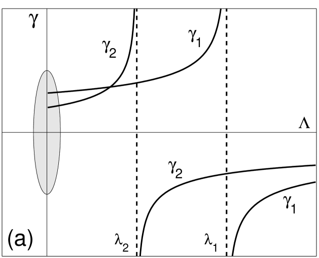
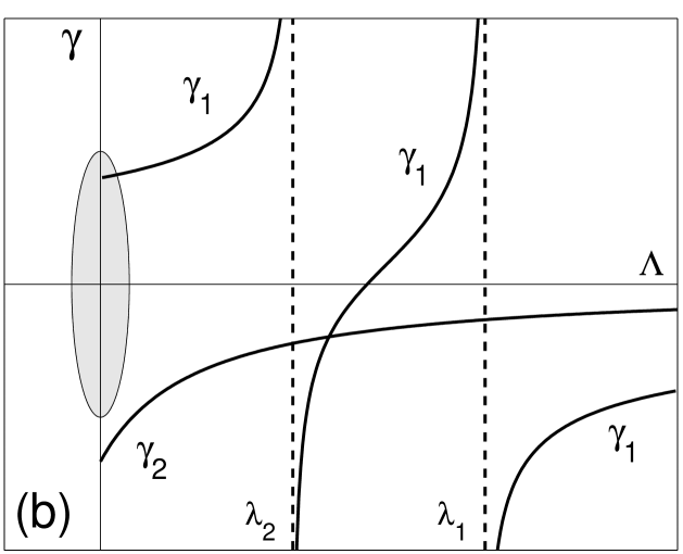
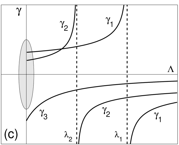
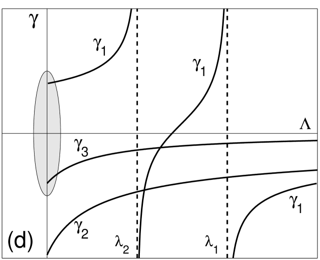
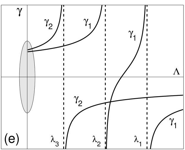
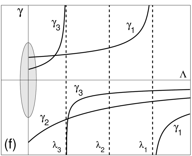
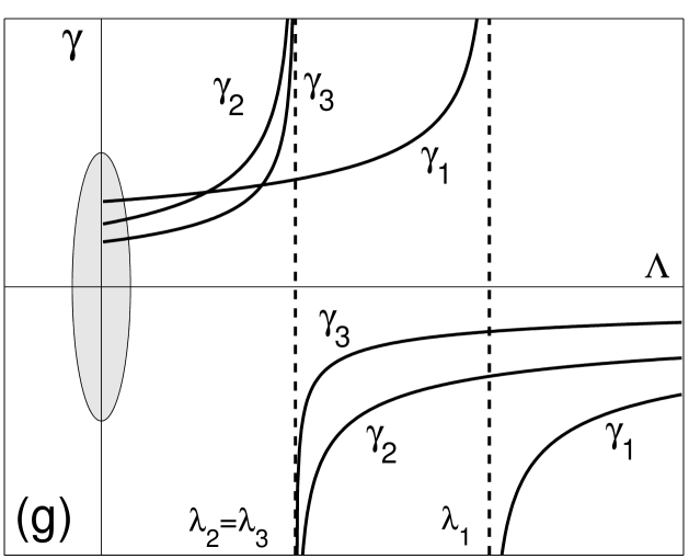
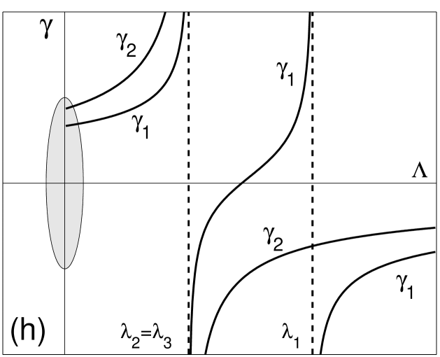
The facts stated in the previous paragraph allow one to specify when can be singular (i.e., one of ) for . We will do so for generic cases first and at the end will consider the missed special cases. One should consider three possibilities:
| (i) , (ii) , (iii) . | (3.14) |
Qualitatively different situations for possibilities (i) and (ii) are examplified by Fig. 1(a–d). From panels (a,c) in this Figure one can see that does not occur for provided that . From Fig. 1(b,d) it also follows that if , then there is always a for some . By inspection, one can convince oneself that these statements are true is the general case (i.e., for any and ) for possibilities (i) and (ii). One can also see that the situation where cannot occur. Indeed, by (3.12), all , and they can become positive only at ’s. Hence the number of positive eigenvalues of cannot exceed the number of positive ’s, which is . Finally, in regards to possibility (iii), one can easily see (Fig. 1(e)) that there should always be a for some . To summarize, does not become singular for positive only when .
Thus, to arrive at conditions (3.1b), we need to relate with . First, in analogy to the first equation in (3.7),
| (3.15) |
As we noted after Eq. (3.2), the right-hand side of (3.15) does not, in general, vanish. We will now find . From the definition of ,
| (3.16) |
On the other hand, consider Eq. (2.8a) written for the transformed operator and note that the last term in that equation is (see also (2.4)). Differentiation of this equation with respect to yields:
| (3.17a) | |||
| where and is the vector whose th entry is 1 and the other entries are zero. Combining Eqs. (3.17a) for all yields | |||
| (3.17b) | |||
where is an matrix. Now, comparison of (3.16) and (3.17b) shows that
| (3.18) |
where are arbitrary constants, and we have used our assumption that the null space of (and hence of ) can consist only of translational-invariance eigenmodes. All such eigenmodes are orthogonal to , as can be seen by considering their inner products with (3.17b). Then the substitution of (3.18) into (3.15) and recalling that (see (2.8b) and (2.12)) yields . Given the arbitrariness of (see the text after (3.8)), this implies that
| (3.19) |
This fact along with the summary sentence found before Eq. (3.15) entails condition (3.1b) in the generic case.
Let us now consider special cases that we have glossed over. First, suppose one of the terms in the discrete sum in (3.7) with a is a zero matrix. This can occur only when . Then by the first equation in (3.4), the corresponding eigenfunction of satisfies the orthogonality condition (2.14) and, by (3.8) and (3.5), is also an eigenfunction of with the eigenvalue . Thus, even though all the eigenvalues of are continuous at and do not change their signs (see Fig. 1(f), where ), operator still has a positive eigenvalue . Note that since fewer than of the eigenvalues change sign as decreases from to , then and hence by (3.19), this special cases falls under the generic condition (3.1b).
Second, suppose that two positive eigenvalues of the self-adjoint operator are the same. Since the corresponding eigenfunctions are linearly independent, so are the eigenvectors of whose eigenvalues will have a pole singularity at . Figures 1(g,h) illustrate two qualitatively different situations that can occur in this case. As one can see, condition (3.1b) still determines whether any of the ’s can vanish for .
Third, suppose is singular. This means that there is an eigenfunction of that satisfies the orthogonality condition (2.14). As we point our below, this may prevent the ITEM and modified CGM from converging. Hence we impose condition (3.1a). Thus, we have established both conditions (3.1b) as being necessary and sufficient to guarantee that the iterative methods (2.9b) (with (1.10) being satisfied) and (A.1f) will converge for any initial guess that is sufficiently close to the solitary wave being sought.
Let us now discuss how these methods may behave if either of these conditions is violated. If (3.1b) does not hold, then the ITEM is guaranteed to diverge for a generic initial condition, since the iteration error will contain a component of the eigenmode that will increase by a factor at each iteration. On the other hand, if (3.1a) is violated, then the iteration error will contain an eigenmode with , which will remain the same at each iteration. Hence the ITEM will settle near , and the norm of the iteration error will not be able to reach an arbitrarily low prescribed error. Thus, the linearized convergence analysis predicts that the method will “stall” at a higher error, but will not diverge. (Taking into account terms nonlinear in (see (1.7)) may yield the information of whether the method actually converges or diverges. However, such a nonlinear analysis is of limited practical use since, even if the ITEM is found to eventually converge, it would do so very slowly in this case.)
As for the modified CGM, it is not bound to diverge if is not negative definite. However, it may do so when either of conditions (3.1b) is violated. The mechanism of this divergence would be the vanishing of the denominator in Eqs. (A.1fb,e) of the algorithm. Such a divergence may perhaps be avoided by choosing a different (but still generic) initial guess .
Finally, let us present an example where one can predict convergence of the ITEM and modified CGM without computing the eigenvalues of and . This example is a straightforward extension of Corollary 1 in [1] to the multi-component case. Consider a system of incoherently coupled NLS-type equations, generalizing (1.2):
| (3.20) |
Its solitary wave is sought in the form with being real. Note that in this case, , , and also
| (3.21a) | |||
| In this case the operator is diagonal with entries | |||
| (3.21b) | |||
Suppose that at least one of the components of has at least one node and is positive (semi)definite. Then , and hence the iterative methods (2.9b) and (A.1f) diverge.
On the other hand, suppose that all components of are nodeless and is negative (semi)definite. Then , and hence the iterative methods converge. The proof of both statements repeats that of Corollary 1 in [1] and hence is not given here.
4 Geometric interpretation of when
In the case of a single equation, the ITEM’s convergence condition in (1.12b) has a simple geometric interpretation: the curve must have a positive slope. (In other words, solitary waves for which and curve has a negative slope cannot be obtained by the ITEM; however, they may be obtained by other iterative methods [1].) The convergence condition in the multi-component case, Eq. (3.1b), is not as straightforward to visualize. In this section we will give a geometric interpretation of this condition for the case , i.e. when the solitary wave has two quadratic conserved quantities and . (Note that the solitary wave in this case can have more than two components: examples include the three-wave system [14, 15] and Eqs. (2.1).) While in the case the Jacobian can be either positive or nonpositive (i.e., there are two possibilities), in the there are three possibilities: when has two, one, or no positive eigenvalues. Thus, below we will give a geometric interpretation of these three situations. Interestingly, this interpretation makes reference of a single curve (see Eqs. (4.5c) below) — an intersection line of surfaces and shifted in a certain manner.
For brevity, let us denote
| (4.1) |
Note that is a symmetric matrix (see (3.7)), and so . From the quadratic equation satisfied by its eigenvalues one can see that:
| (4.2a) | |||
| (4.2b) | |||
| (4.2c) |
We have used the symmetry of to infer that a definite sign of in (4.2ca,c) implies the corresponding sign for both these diagonal entries individually.
Let us consider two surfaces and and the normal vectors to them at a given point :
| (4.3) |
where these vectors are chosen to point downward. If these surfaces are vertically shifted so as to have the same height at point , then the cross-product of the normal vectors defines the direction of the intersection line of such shifted surfaces at this point. The vertical component of this cross-product is :
| (4.4) |
Thus, according to the above definition, the intersection line, , of the shifted surfaces and points in the same vertical direction (i.e., up or down) as . Let us also note that are the projections of onto the axes and . With these observations, conditions (4.2c) are restated as:
| (4.5a) | |||
| (4.5b) | |||
| (4.5c) |
Finally, let us note that conditions (4.5c) can be restated solely in terms of the two-component vectors obtained by projection of on the horizontal plane:
| (4.6a) | |||
| (4.6b) | |||
| (4.6c) |
where the angle is measured from to in the counterclockwise direction.
5 Connection between convergence and dynamical stability
First, we observe that the conditions (3.1b) under which the ITEM (2.9b) and the modified CGM (A.1f) are guaranteed to converge [18] are the same under which the solitary wave of the incoherently coupled NLS-type equations (3.20) with all nodeless components is linearly stable [12]. (More precisely, the system analyzed in [12] had , but the results of that paper are straightforwardly extended to apply to (3.20).) Thus, the nodeless solutions of (3.20) found by the iterative methods of this paper are guaranteed to be dynamically linearly stable. This is an extension of the result found in [1] for a single-component Eq. (1.2).
Let us now explain why this close connection between the convergence and stability takes place. Our explanation applies both to single- and multi-component equations. In regards to the convergence conditions, recall that the iteration methods converge when the operator in (2.10) is negative definite on the space of functions satisfying the orthogonality relation (2.11). Note that on this space, , and therefore, the negative definitenesses of and are equivalent under (2.11).
Let us now turn to the stability conditions. The details are slightly different for envelope and carrier solitary waves, so we begin with the former using Eqs. (2.1) as an example whenever needed. Seeking the slightly perturbed solitary wave in the form similar to (2.3) where now all are replaced by
| (5.1) |
one obtains (see, e.g., [12]):
| (5.2) |
In the case of Eqs. (2.3) or (3.20), (see (2.8a)), but in general (e.g., for the three-wave system [14, 15]) this is not so. Also, in the case where , it is convenient, although not critical, to write the -term in as, e.g., for (2.4): diag; this makes explicitly self-adjoint. What is important is that
| (5.3) |
where the right-hand side is the zero matrix. Condition (5.3) is, in fact, the solvability condition of the second equation in (5.2), and is equivalent to the condition that satisfy the orthogonality relation (2.11):
| (5.4) |
Property (5.4) is easily verified by substituting (5.1) into the conservation law .
By (5.4), (5.3) one can invert the second equation in (5.2) and substitute the result in the first equation:
| (5.5) |
Recall that this generalized eigenvalue problem is considered on the restricted space (5.4). Both operators in (5.5) are self-adjoint. Then, if (and hence ) is negative definite, then by Sylvester’s law of inertia, the sign of is determined by the signs of the eigenvalues of . If L is negative definite (again — on the restricted space (5.4), or equivalently, (2.11)), then and hence the solitary wave is dynamically linearly stable (see (5.1)).
Thus, to summarize: The conditions of convergence of the ITEM and modified CGM coincide with the conditions under which the solitary wave is dynamically linearly stable if and only if operator is negative definite. In particular, this occurs when is a ground state. (Unfortunately, the latter fact is not readily determined by inspection for multi-component solitary waves.) Let us note that this result about the coincidence of convergence and stability conditions for ground-state solitary waves fully agrees with the results of [4, 19], where it was proven that an ITEM-like method converges to ground states of (1.2) and its generalization (3.20) describing dynamics of Bose–Einstein condensates.
Finally, we give a counterpart of the above statement for carrier wave equations using the KdV equation
| (5.6) |
as an example. Its solitary wave with velocity satisfies an equation , whose linearized operator is . The iterative methods seeking a solitary wave with a prescribed value of power (1.1) will converge provided that is negative definite on a space of functions satisfying a variant of (2.11):
| (5.7) |
On the other hand, the stability analysis of (5.6) via an ansatz leads to the eigenvalue problem . Upon the substitution , this eigenvalue problem is rewritten in the same form as (5.2) [20]:
| (5.8) |
Note that due to the translational invariance of the solitary wave, is a solution of . Thus, all considerations for the envelope equations carry over to the case of (5.6), and we conclude that the convergence conditions of the ITEM and CGM coincide with the stability conditions of the solitary wave if is the ground state of (or, equivalently, is negative definite on the space defined by (5.7)).
It may also be pointed out that in coupled multi-component generalizations of the KdV, there is only one parameter — the wave’s velocity — that is the analog of the propagation constant vector for the envelope equations, like in (2.1) or (3.20). Therefore, in this case, there is only one quadratic conserved quantity (which is probably the sum of the powers of all the components). In other words, , and hence the ITEM and modified CGM can converge only if .
6 Conclusions
In this work, we obtained the convergence conditions of the iterative methods (2.9b) and (A.1f) that find multi-component solitary waves with prescribed values of quadratic conserved quantities (2.6). These convergence conditions are given by (3.1b) (provided that (1.10) holds for the ITEM (2.9b)), which extend the convergence conditions of the single-component ITEM obtained in [1]. These conditions also turn out to be the same as the dynamical stability conditions for the nodeless (e.g., ground-state) solitary wave of the system of incoherently coupled NLS-type equations (3.20), which were obtained in [12]. For a single-component NLS-type equation (1.2), such a coincidence was observed in [1]. Earlier, similar statements were proven for (1.2) and (3.20) in [4, 19] by different techniques. In Section 5 we showed that, in general, the convergence conditions of the iterative methods (2.9b) and (A.1f), on one hand, and the dynamical stability conditions, on the other, coincide for ground-state solitary waves of all Hamiltonian nonlinear wave equations.
Let us conclude with two remarks. First, even though we stated the ITEM (2.9b) in the main text of the paper while stating the CGM (A.1f) in Appendix, we remind the reader (see Section 2) that if the ITEM converges slowly, then the modified CGM will provide considerable acceleration of the iterations. Alternatively, one can use the slowest mode elimination technique [21] to accelerate the algorithm of the ITEM. Comparison of these three methods was done in [11], with the modified CGM being found the fastest.
Second, above we have explicitly mentioned the form of the operators employed by the ITEM and modified CGM for envelope equations (like (2.1) and (3.20)) and for the carrier waves (like the KdV, (5.6)). For systems that couple envelope and carrier waves, which are commonly referred to as short–long wave interaction, or generalized Zakharov–Benney, equations, the formalism remains the same.
Appendix: Modified CGM for solitary waves with a prescribed
The steps of this algorithm for Eq. (2.8a) are (operator is defined in (2.10)):
| (A.1a) | |||
| (A.1b) | |||
| (A.1c) | |||
| (A.1d) | |||
| (A.1e) | |||
| (A.1f) |
Equation (A.1a) defines the initial residual and the search direction . The first equation in (A.1c) updates the iterative solution along the search direction by making a “step” of “length” found in (A.1b). Equations (A.1fd,f) update the residual and the search direction using an auxiliary parameter computed in (A.1e).
References
- [1] J. Yang and T.I. Lakoba, “Accelerated imaginary-time evolution methods for the computation of solitary waves,” Stud. Appl. Math. 120, 265–292 (2008).
- [2] M.L. Chiofalo, S. Succi, and M.P. Tosi, “Ground state of trapped interacting Bose-Einstein condensates by an explicit imaginary-time algorithm,” Phys. Rev. E 62 7438–7444 (2000).
- [3] J.J. Garcia-Ripoll and V.M. Perez-Garcia, “Optimizing Schrödinger functionals using Sobolev gradients: Applications to Quantum Mechanics and Nonlinear Optics,” SIAM J. Sci. Comput. 23, 1316–1334 (2001).
- [4] W. Bao and Q. Du, “Computing the ground state solution of Bose–Einstein condensates by a normalized gradient flow,” SIAM J. Sci. Comput. 25, 1674–1697 (2004).
-
[5]
V.S. Shchesnovich and S.B. Cavalcanti, “Rayleigh functional for nonlinear systems,”
available at
http://www.arXiv.org, Preprint nlin.PS/0411033. - [6] In the language of Linear Algebra, differs from by a rank-one correction (i.e., the last term in (1.8)), and the relation between the eigenvalues of two such matrices can be found, e.g., in [7], p. 230.
- [7] L.N. Trefethen and D. Bau, III, Numerical Linear Algebra, SIAM, Philadelphia, 1997.
- [8] N.G. Vakhitov and A.A. Kolokolov, “Stationary solutions of the wave equation in the medium with nonlinearity saturation,” Radiophys. Quantum Electron. 16, 783–789 (1973); A.A. Kolokolov, “Stability of stationary solutions of nonlinear wave equations,” Radiophys. Quantum Electron. 17, 1016–1020 (1974)
- [9] In [1] it was also required that for , the eigenfunction of corresponding to the positive eigenvalue be not orthogonal to . However, one can show, similarly to how we will do it in Section 3, that this special case actually falls under case (1.12b).
- [10] J. Yang and T.I. Lakoba, “Universally-convergent squared-operator iteration methods for solitary waves in general nonlinear wave equations,” Stud. Appl. Math. 118, 153–197 (2007).
-
[11]
T.I. Lakoba, “Conjugate gradient method for finding fundamental solitary waves,” to appear in Physica D
(2009); also available at
http://www.arXiv.org, Preprint 0903.3266. - [12] D.E. Pelinovsky and Y.S. Kivshar, “Stability criterion for multicomponent solitary waves,” Phys. Rev. E 62, 8668–8676 (2000).
- [13] T.I. Lakoba, D.J. Kaup, and B.A. Malomed, “Solitons in nonlinear directional coupler with two orthogonal polarizations,” Phys. Rev. E 55, 6107–6120 (1997).
- [14] Y. N. Karamzin and A. P. Sukhorukov, “Mutual focusing of high-power light beams in media with quadratic nonlinearity,” Sov. Phys. JETP 41, 414–420 (1976).
- [15] A.V. Buryak, P. Di Trapani, D.V. Skryabin, and S. Trillo, “Optical solitons due to quadratic nonlinearities: From basic physics to futuristic applications,” Phys. Rep. 370, 63–235 (2002).
- [16] R. Horn and C. Johnson, Matrix Analysis, Cambridge University Press, 1991. [Specifically, see Theorems 4.5.8 and 7.6.3.]
- [17] While many pieces of the analysis of this section can be found in [12], we found it expedient to write a self-contained account of it. Indeed, it would take one some effort to relate the two quite different setting and notations of that paper and this work. Even more nontrivial effort is needed to deduce the main result, Eqs. (3.1b), of this work from the main results summarized in Section II of [12].
- [18] Recall that we always imply that (1.10) holds for the ITEM.
- [19] W. Bao, “Ground states and dynamics of multi-component Bose-Einstein condensates,” Multiscale Model. Simul. 2, 210–236 (2004).
- [20] Y. Kodama and D. Pelinovsky, “Spectral stability and time evolution of N-solitons in the KdV hierarchy,” J. Phys. A: Math. Gen. 38, 6129–6140 (2005).
- [21] T.I. Lakoba and J. Yang, “A mode elimination technique to improve convergence of iteration methods for finding solitary waves,” J. Comp. Phys. 226, 1693–1709 (2007).