A VLT VIMOS integral field spectroscopic study of perturbed blue compact galaxies: UM 420 and UM 462

Abstract

We report on optical integral field spectroscopy of two unrelated blue compact galaxies mapped with the 13 $\times$ 13 arcsec² VIMOS integral field unit at a resolution of 0.33 $\times$ 0.33 arcsec². Continuum and background subtracted emission line maps in the light of [O iii] $\lambda$5007, H$\alpha$, and [N ii] $\lambda$6584 are presented. Both galaxies display signs of ongoing perturbation and/or interaction. UM 420 is resolved for the first time to be a merging system composed of two starbursting components with an ‘arm-like’ structure associated with the largest component. UM 462 which is a disrupted system of irregular morphology is resolved into at least four starbursting regions. Maps of the H$\alpha$ radial velocity and FWHM are discussed. No underlying broad line region was detected from either galaxy as the emission lines are well-fitted with single Gaussian profiles only. Electron temperatures and densities as well as the abundances of helium, oxygen, nitrogen, and sulphur were computed from spectra integrated over the whole galaxies and for each area of recent star formation. Maps of the O/H ratio are presented: these galaxies show oxygen abundances that are $\sim$ 20 per cent solar. No evidence of substantial abundance variations across the galaxies that would point to significant nitrogen or oxygen self-enrichment is found ($\lesssim$ 0.2 dex limit). Contrary to previous observations, this analysis does not support the classification of these BCGs as Wolf-Rayet galaxies as the characteristic broad emission line features have not been detected in our spectra. Baldwin-Phillips-Terlevich emission line ratio diagrams which were constructed on a pixel by pixel basis indicate that the optical spectra of these systems are predominantly excited by stellar photoionization.

1 Introduction

Blue compact dwarf galaxies (BCGs) offer a means of exploring star-formation in low-mass, low-metallicity (1/50–1/3 Z_⊙,Kunth:2000) systems and, by analogy, the chemically un-evolved systems in the high-$z$ primordial universe. Typically, they are characterised by their strong emission lines superimposed on a faint, blue continuum, resulting from one or more recent bursts of star-formation. These compact, gas-rich objects are estimated to have high star-formation rates in the order of 0.1 to 1 M_⊙ yr^-1 (Fanelli:1988) with typical H i masses of M${}_{HI}\sim 10^{7}-10^{8}$ M_⊙ (Thuan:1981), and are ideal laboratories for many topics related to star-formation, partly because they do not display more complicated phenomena, such as density waves, that operate in larger galaxies (Cairos:2001). This is a study of two BCGs, UM 420 and UM 462, first discovered by the University of Michigan survey for extragalactic emission-line objects (Macalpine:1978). Their individual properties may provide insights into the role of galaxy interactions in chemical recycling and starbursting episodes. Several studies have suggested that interactions with other systems are a contributing factor to large-scale starbursts in dwarf galaxies (Brinks:1990; Mendez:2000; Iglesias:2001; Verdes:2002; Tran:2003). Hence it may be no coincidence that both galaxies studied here display signs of interaction and/or perturbation in the form of tails, multiple nuclei, or disrupted morphology.

UM 420 was reported by Lopez-Sanchez:2008 as having an irregular and elongated morphology, with two long regions extending in different directions from the brightest central region. A bright spiral galaxy, UGC 1809, lies 16.5^′′ west of UM 420, but at less than half the redshift of UM 420 is not physically associated to it and cannot cause an effect. UM 420 was once thought to be a large H ii region near the edge of UGC 1809’s spiral arms, and as a result the SIMBAD data base currently incorrectly lists its RA and DEC as those of UCG 1809 (the correct RA and DEC for UM 420 are given in Table LABEL:tab:galaxies). Pustilnik:2004 describe UM 420 as being a possible ‘sinking merger’, i.e. harbouring a satellite galaxy that is sinking into a larger, gas-rich companion.

UM 462 with UM 461 form part of an interacting binary pair separated by only $\sim$50^′′ (Taylor:1995; Telles:1995). In a H i survey of H ii galaxies with companions (Taylor:1995), UM 461 was observed to have a tidal arm extending in the direction of UM 462 and outer H i contours that are clearly disturbed by its nearby neighbour. Telles:1995 interpreted UM 462 as being part of a group of H ii galaxies, UM 461, UM 463 and UM 465, whose star-bursting episodes are synchronised on time scales of less than 10⁷ years, despite being separated by $\sim$1–2 Mpc. Following the classification system of Loose:1985, Cairos:2001 classified UM 462 as being of ‘iE’ type, i.e. showing a complex inner structure with several star-forming regions superimposed on an extended regular envelope. This type of structure is commonly interpreted as a sign of interaction. Spectroscopically, both galaxies have been classified as Wolf-Rayet (WR) galaxies (this is however disputed in the present work; see Sec. 5.3), with broad He ii $\lambda$4686 being detected in their spectra (Izotov:1998; Guseva:2000). Guseva:2000 also claimed to see broad C iv $\lambda$4658 and C iv $\lambda$5808 emission in the spectra of UM 420, indicating the presence of WCE stars, although the detections were doubted by Schaerer:1999 on the basis of the S/N ratio of the Guseva:2000 spectrum. The relative numbers of WR stars to O-type stars were estimated by Guseva:2000 as 0.03 and 0.005 for UM 420 and UM 462, respectively. Schaerer:1999 have defined WR galaxies as being those whose ongoing or recent star formation has produced stars sufficiently massive to evolve to the WR stage. However, the same authors also note that the definition of a WR galaxy is dependent on the quality of the spectrum, and the location and size of the aperture.

UM 420 falls within a small sub-set of BCGs reported by Pustilnik:2004 as having anomalously high N/O ratios ($\sim$ 0.5 dex) compared to BCGs of similar oxygen metallicity (12+log(O/H)=7.93; Izotov:1998, IT98 hereafter). They attributed this over-abundance of nitrogen to the effects of N-rich winds from large numbers of Wolf-Rayet (WNL-type) stars. A previous IFU study by James:2009 (J09 hereafter) of another BCG in this ‘high N/O’ group, Mrk 996, derived a significantly higher O/H ratio than previously and an N/O ratio for its narrow-line component which is now typical for its metallicity. Mrk 996, however, was shown by J09 to also contain an extremely dense, extended broad-line component displaying a N/O ratio up to 20 times higher than the galaxy’s narrow-line component; this large N/H and N/O enrichment was attributed to the cumulative effects of a large population of $\sim$2600 WNL-type stars whose number was estimated from fitting the broad emission features at 4640 and 4650-Å with theoretical WR spectral templates. By conducting a similar study of UM 420 we aimed to investigate its N/O ratio status, and to study potential effects to the gas abundance patterns due to WR stars. On the other hand, UM 462 provides a useful comparison, as it has been reported to have a rather normal N/O ratio close to the average observed for many BCGs at its published metallicity of 12 $+$ log(O/H) $=$ 7.95 (IT98).

In order to understand interaction-induced starbursts, it is essential to gain spatial information regarding the properties (e.g. physical conditions, chemical abundances) of the starburst regions and any spatial correlations that may hold. This type of information has been limited in previous long-slit spectroscopic studies of H ii galaxies. In this paper we present high resolution optical observations obtained with the VIMOS integral field unit (IFU) spectrograph on the ESO 8.2m Very Large Telescope UT3/Melipal. The data afford us new spatiokinematic ‘3-D’ views of UM 420 and UM 462. The spatial and spectral resolutions achieved (Section 2.1) allow us to undertake a chemical and kinematical analysis of both systems, providing a clearer picture of the ionised gas within their star-forming regions. We adopt distances of 238 Mpc and 14.4 Mpc for UM 420 and UM 462, respectively, corresponding to their redshifted velocities measured here of $+$17,454 and $+$1057 km s^-1 ($z$ $=$ 0.060604 and 0.003527, as given in Table LABEL:tab:galaxies), for a Hubble constant of H_o = 73.5 km s^-1 Mpc^-1 (Bernardis:2008).

Table 1: General Parameters of UM 420 and UM 462

	Coordinates (J2000)
Name	$\alpha$	$\delta$	$z$a	Distance (Mpc)	Other Names
UM 420	02 21 36.2	00 29 34.3	0.060604	238
UM 462	11 53 18.5	-02 32 20.6	0.003527	14.4	Mrk 1307, UGC 06850

^a

Derived from the present observations

2 VIMOS IFU Observations and Data Reduction

2.1 Observations

Two data sets for each galaxy were obtained with the Visible Multi-Object Spectrograph (VIMOS) IFU mounted on the 8.2m VLT at the Paranal Observatory in Chile. All data sets were taken with the high-resolution and high-magnification settings of the IFU, which resulted in a field-of-view (FoV) of 13${}^{\prime\prime}\times$13^′′ covered by 1600 spaxels (spatial pixels) at a sampling of 0.33^′′ per spaxel. The data consist of high-resolution blue grism spectra (HRblue, $\sim$0.51 Å/pixel, 2.01$\pm$ 0.23 Å FWHM resolution) covering 4150–6200 Å and high-resolution orange grism spectra (HRorange, $\sim$0.6 Å/pixel, 1.92 $\pm$ 0.09 Å FWHM resolution) covering 5250–7400 Å. Spectra from both grisms for each galaxy are shown in Figure 1. The observing log can be found in Table LABEL:tab:obslog. Four exposures were taken per grism, per observation ID. The third exposure within each set was dithered by $+$0.25^′′ in RA and by $+$0.61^′′ in DEC for both galaxies (corresponding to a 2 spaxel offset in the $X$-direction) in order to remove any broken fibres when averaging exposures. All observations were taken at a position angle of 20^∘ for UM 420 and 22^∘ for UM 462.

Table 2: VIMOS IFU observing log

Observation ID	Date	Grism	Exp. time (s)	Airmass range	FWHM seeing (arcsec)
UM 420
250536-9	14/11/2006	HR blue	4 ${\times}$ 402	1.11–1.40	0.85
250534,250535	14/11/2006	HR orange	4 ${\times}$ 372	1.13–1.36	0.79
UM 462
250563-6	22-23/03/2007	HR blue	4 ${\times}$ 402	1.60 – 1.10	1.02
250559,250562	22-23/03/2007	HR orange	4 ${\times}$ 372	2.16 – 1.73	0.74

2.2 Data Reduction

Data reduction was carried out using the ESO pipeline via the gasgano software package and followed the sequence outlined by J09. The reduction involves three main tasks: vmbias, vmifucalib and vmifustandard. The products of these were fed into vmifuscience which extracted the bias-subtracted, wavelength- and flux-calibrated, and relative fibre transmission-corrected science spectra. The final cube construction from the quadrant-specific science spectra output by the pipeline utilised an IFU table that lists the one to one correspondence between fibre positions on the IFU head and stacked spectra on the IFU (Bastian:2006). A final data cube for each of the HRblue and HRorange grisms was then created by averaging over the final flux-calibrated science cubes created from each observation block. For a more detailed description of the data reduction and processing from science spectra to spatially reconstructed cube, see J09. A schematic representation of the data reduction processes performed within gasgano is provided by Zanichelli:2005. Sky subtraction was performed by locating a background region within each quadrant, summing the spectra over each of the spaxels in the reconstructed cube and subtracting the median sky spectrum of the region from its corresponding quadrant. Median combining was needed to ensure that any residual contamination from faint objects was removed. In the case of UM 420, the western edge of the IFU frame sampled the outermost faint regions of the unrelated foreground spiral galaxy UGC 1809 (e.g. Lopez-Sanchez:2008), and this background subtraction procedure enabled the removal of any contaminating signal. Before averaging to produce a final data cube for each grism, each cube was corrected for differential atmospheric refraction (DAR). This correction accounts for the refraction of an object’s spectrum along the parallactic angle of the observation as it is observed through the atmosphere. The cubes were corrected using an iraf-based programme written by J. R. Walsh (based on an algorithm described in Walsh:1990). The procedure calculates fractional spaxel shifts for each monochromatic slice of the cube relative to a fiducial wavelength (i.e. a strong emission line), shifts each slice with respect to the orientation of the slit on the sky and the parallactic angle and recombines the DAR-corrected data cube. For both galaxies a high S/N ratio fiducial emission line (He i $\lambda$5876) was available within the wavelength overlap of the HRblue and HRorange cubes. Although not essential, correcting multiple spectral cubes to a common emission line allows one to check that the alignment between them is correct.

2.3 Emission Line Profile Fitting

Taking into account that there are 1600 spectra across the FoV of each data cube, we utilised an automated fitting process called PAN (Peak ANalysis; Dimeo:2005). This is an IDL-based general curve-fitting package, adapted by Westmoquette:2007 for use with FITS data. The user can interactively specify the initial parameters of a spectral line fit (continuum level, line peak flux, centroid and width) and allow PAN to sequentially process each spectrum, fitting Gaussian profiles accordingly. The output consists of the fit parameters for the continuum and each spectral line’s profile and the $\chi^{2}$ value for the fit. It was found that all emission lines in the spectra of both UM 420 and UM 462 could be optimally fitted with a single narrow Gaussian. For high S/N ratio cases, such as Balmer lines and [O iii] $\lambda$5007, attempts were made to fit an additional broad Gaussian profile underneath the narrow component. These fits were assessed using the statistical F-test procedure, a process that determines the optimum number of Gaussians required to fit each line (see J09 for a more detailed discussion). We found that it was not statistically significant to fit anything more than a single Gaussian to the emission lines in the spectra of either object. Thus single Gaussian profiles were fitted to each emission line profile, restricting the minimum FWHM to be the instrumental width. Suitable wavelength limits were defined for each emission line and continuum level fit. Further constraints were applied when fitting the [S ii] doublet: the wavelength difference between the two lines was taken to be equal to the redshifted laboratory value when fitting the velocity component, and their FWHM were set equal to one another. The fitting errors reported by PAN underestimate the true uncertainties. We thus follow the error estimation procedure outlined by J09, which involves the visual re-inspection of the line profile plus fit after checking which solution was selected by our tests, and taking into account the S/N ratio of the spectrum. By comparing PAN fits to those performed by other fitting techniques (e.g. iraf’s splot task) on line profiles with an established configuration (i.e. after performing the F-test) we find that estimated uncertainties of $\sim$5–10 per cent are associated with the single Gaussian fits. A listing of the measured flux and FWHM uncertainties appears in Table LABEL:tab:fluxes, where errors are quoted for individual component fits to emission lines detected on the integrated spectra from across all of UM 420 and UM 462.

3 Mapping Line Fluxes

3.1 Line fluxes and reddening corrections

Figure 1: VIMOS IFU summed spectra of UM 420 after smoothing with a 5 pixel boxcar function: (a) UM 420, top panel: high resolution blue spectrum, bottom panel: high resolution orange spectrum. The spectra are integrated over an area of 7.6${}^{\prime\prime}\times$6.3^′′ (8.8$\times$7.2 kpc²) and correspond to exposure times of 4$\times$402 s and 4$\times$372 s for the HRblue and HRorange grisms, respectively; (b) Same as (a), for UM 462. Spectra are integrated over an area of 10.2${}^{\prime\prime}\times$10.2^′′ (714.1$\times$714.1 pc²).

Full HRblue and HRorange spectra for UM 420 and UM 462 are shown in Figure 1(a) and (b), respectively. Table LABEL:tab:fluxes lists the measured FWHMs and observed and de-reddened fluxes of the detected emission lines within UM 420 and UM 462, respectively. The listed fluxes are from IFU spectra summed over each galaxy and are quoted relative to $F$(H$\beta$) $=$ 100.0. Foreground Milky Way reddening values of $E$($B-V$) $=$ 0.04 and 0.02 were adopted, from the maps of Schlegel:1998, corresponding to $c$(H$\beta$) $=$ 0.05 and 0.03 in the directions of UM 420 and UM 462, respectively. The line fluxes were then corrected for extinction using the Galactic reddening law of Howarth:1983 with $R_{V}$ $=$ 3.1 using $c$(H$\beta$) values derived from each galaxy’s H$\alpha$/H$\beta$ and H$\gamma$/H$\beta$ emission line ratios, weighted in a 3 : 1 ratio, respectively, after comparison with the theoretical Case B ratios from Hummer:1987 of $j_{\rm H\alpha}/j_{\rm H\beta}$ $=$ 2.863 and $j_{\rm H\gamma}/j_{\rm H\beta}$ $=$ 0.468 (at $T_{\rm e}$ $=$ 10⁴ K and $N_{\rm e}$ $=$ 100 cm^-3). The same method was used to create $c$(H$\beta$) maps for each galaxy, using H$\alpha$/H$\beta$ and H$\gamma$/H$\beta$ ratio maps, which were employed to deredden other lines on a spaxel by spaxel basis prior to creating electron temperature, electron density and abundance maps. As stated in Table LABEL:tab:fluxes, overall $c$(H$\beta$) values of 0.25$\pm$0.08 and 0.19$\pm$0.04 were found to be applicable to the integrated emission from UM 420 and UM 462, respectively.

Table 3: Emission line measurements for summed spectra of UM 420 and UM 462. Observed and de-reddened fluxes are relative to F(H$\beta$)=I(H$\beta$)=100. Line fluxes were extinction-corrected using the c(H$\beta$) values shown at the bottom of the table, calculated from the relative H$\alpha$, H$\beta$ and H$\gamma$ fluxes. FWHMs have been corrected for the instrumental FWHM resolution (Section 2.1)

	UM 420			UM 462
Line ID	FHWM (km s-1)	F($\lambda$)	I($\lambda$)	FHWM (km s-1)	F($\lambda$)	I($\lambda$)
3969 [Ne III]	431.0$\pm$ 52.2	27.1$\pm$ 2.5	30.5$\pm$ 2.8	—	—	—
4101 H$\delta$	205.7$\pm$ 12.1	22.8$\pm$ 1.2	25.3$\pm$ 1.3	—	—	—
4340 H$\gamma$	183.3$\pm$ 5.3	42.0$\pm$ 1.1	45.1$\pm$ 1.1	143.1$\pm$ 1.8	43.3$\pm$ 0.5	45.7$\pm$ 0.5
4363 [O III]	239.1$\pm$ 64.0	6.3$\pm$ 1.3	6.8$\pm$ 1.4	156.6$\pm$ 13.8	7.1$\pm$ 0.5	7.4$\pm$ 0.5
4471 He I	143.5$\pm$26.3	3.5$\pm$0.5	3.7$\pm$0.5	113.7$\pm$ 12.4	3.1$\pm$ 0.3	3.2$\pm$ 0.3
4686 He II	—	—	—	175.4$\pm$ 5.1	1.7$\pm$ 0.1	1.7$\pm$ 0.1
4861 H$\beta$	187.9$\pm$ 2.0	100.0$\pm$ 1.3	100.0$\pm$ 0.9	123.4$\pm$ 0.7	100.0$\pm$ 0.7	100.0$\pm$ 0.5
4921 He I	—	—	—	122.5$\pm$ 7.3	0.9$\pm$ 0.2	0.9$\pm$ 0.2
4959 [O III]	182.3$\pm$ 1.8	139.2$\pm$ 1.7	137.3$\pm$ 1.1	118.6$\pm$ 1.2	164.6$\pm$ 1.7	162.9$\pm$ 1.5
5007 [O III]	181.4$\pm$ 1.0	430.5$\pm$ 4.5	421.9$\pm$ 1.9	116.4$\pm$ 0.7	477.4$\pm$ 3.5	470.2$\pm$ 2.5
5015 He I or [FeIV]	—	—	—	104.2$\pm$ 6.6	1.8$\pm$ 0.1	1.8$\pm$ 0.1
5030 [Fe IV]	79.9$\pm$ 15.2	3.5$\pm$ 0.5	3.4$\pm$ 0.5	—	—	—
5876 He I	184.0$\pm$ 14.4	13.2$\pm$ 0.9	11.7$\pm$ 0.7	115.8$\pm$ 11.6	12.1$\pm$ 1.0	11.0$\pm$ 0.9
6051 [Fe IV]	36.7$\pm$ 7.2	6.8$\pm$ 0.4	5.9$\pm$ 0.3	—	—	—
6300 [O I]	—	—	—	116.8$\pm$ 17.2	5.0$\pm$ 0.6	4.4$\pm$ 0.5
6312 [S III]	—	—	—	123.6$\pm$ 21.9	1.9$\pm$ 0.4	1.7$\pm$ 0.3
6363 [O I]	—	—	—	150.9$\pm$ 28.8	3.5$\pm$ 0.7	3.1$\pm$ 0.6
6548 [N II]	238.3$\pm$ 56.6	10.9$\pm$ 2.1	9.1$\pm$ 1.7	127.3$\pm$ 13.5	3.1$\pm$ 0.3	2.7$\pm$ 0.2
6563 H$\alpha$	178.8$\pm$ 1.1	334.4$\pm$ 3.6	279.1$\pm$ 1.4	103.1$\pm$ 0.6	323.4$\pm$ 2.5	282.2$\pm$ 1.6
6584 [N II]	189.7$\pm$ 14.4	29.5$\pm$ 1.8	24.6$\pm$ 1.5	109.8$\pm$ 4.2	8.5$\pm$ 0.3	7.4$\pm$ 0.2
6678 He I	135.7$\pm$105.2	4.7$\pm$1.6	3.8$\pm$1.3	127.6$\pm$ 6.3	4.2$\pm$ 0.4	3.7$\pm$ 0.3
6716 [S II]	196.5$\pm$ 9.3	33.9$\pm$ 1.4	27.9$\pm$ 1.1	101.0$\pm$ 5.2	19.0$\pm$ 0.8	16.4$\pm$ 0.7
6731 [S II]	201.2$\pm$ 12.6	26.9$\pm$ 1.4	22.1$\pm$ 1.1	105.9$\pm$ 7.4	14.4$\pm$ 0.8	12.4$\pm$ 0.7
7136 [Ar III]	—	—	—	104.6$\pm$ 8.9	9.2$\pm$ 0.6	7.8$\pm$ 0.5
c(H$\beta$) dex	0.25$\pm$0.08			0.19$\pm$0.04
F(H$\beta$)$\times$10-16erg s-1 cm-2	359.1$\pm$6.1			2660$\pm$14

3.2 H$\alpha$ line properties

Here we discuss the appearance of the targets in the light of the highest S/N ratio H i emission line, H$\alpha$. Figure 2 shows flux, radial velocity and FWHM maps for H$\alpha$ from UM 420 and UM 462, respectively.

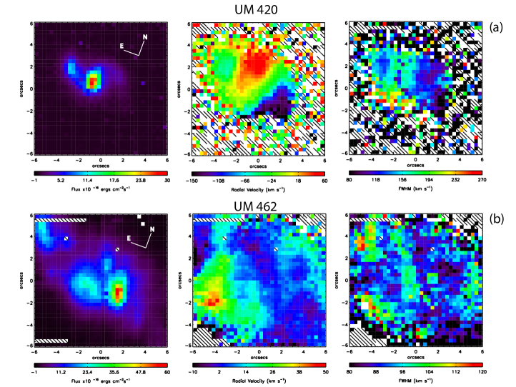
Figure 2: Maps of UM 420 (a) and UM 462 (b) in H$\alpha$; left column: flux per 0.33 arcsec² spaxel; centre column: radial velocity (relative to heliocentric systemic velocity of $+$17,545 and $+$1057 km s^-1 for UM 420 and UM 462, respectively; right column: H$\alpha$ FWHM corrected for the instrumental point spread function. See text for details.

3.2.1 UM 420

The H$\alpha$ flux map shown in the left-hand panel of Figure 2(a) displays a double peak; the first peak is centrally located at the RA and DEC listed in Table LABEL:tab:galaxies, with a surface brightness of 2.75$\times$10^-14 erg cm^-2 s^-1 arcsec^-2 and the second peak is located $\sim$2.2^′′ east of that central position, with a peak surface brightness of 9.72$\times$10^-15 erg cm^-2 s^-1 arcsec^-2. These two H$\alpha$ peaks provide the basis for defining two main star-forming regions, as displayed in Figure 3. An arm-like structure can be seen north-west of the central peak, extending in a south-westerly direction; it could be the result of an ongoing merger or interaction between the two identified regions. A more luminous spiral galaxy, UGC 1809, lies 16.5^′′ westward of the galaxy, as noted by Takase:1986, but at less than half the redshift of UM 420 it cannot be identified as an interacting companion. The VIMOS IFU H$\alpha$ flux is a factor of 1.1 larger than the one measured by IT98 in a 3^′′ $\times$ 200^′′ slit and a factor of 1.8 times larger than that estimated by Lopez-Sanchez:2008 from broad band H$\alpha$ $+$ [N ii] images. The H$\alpha$ radial velocity map shown in the central panel of Figure 2 shows two separate velocity gradients. Firstly, there is a balanced velocity gradient at position angle (PA) 50^∘ east of north (labelled as ‘Position 1’ on the central panel of Figure 4). This linear velocity gradient may be indicative of solid body rotation between the main emission peak (Region 1) and the ‘arm-like’ structure north-west of Region 1. Secondly, the main body of the galaxy, i.e. the double peaked emission structure, shows a velocity gradient at a PA of 110^∘ east of north (labelled as ‘Position 2’ on the central panel of Figure 4).

Figure 4 shows position-velocity (P-V) diagrams along both these axes. These diagrams were created by placing a spaxel-wide (i.e. with a width of 0.33^′′) pseudo-slit across the radial velocity map, and plotting the radial velocity as a function of distance from the slit’s centre. The smooth and symmetrically structured velocity gradient along Position 1 suggests that the axis orthogonal to it could be adopted as a rotational axis for UM 420 (projected on the plane of the sky). From the top panel of Figure 4 we can then make a new estimate of the heliocentric systemic velocity of UM 420; a radial velocity of $+$17,545$\pm$30 km s^-1 is needed to normalise the distribution along the proposed axis of rotation to zero (cf. the $+$17,514$\pm$12 km s^-1 estimation of IT98). Thus a velocity gradient ranging from $\sim$-100 km s^-1 to $\sim$+100 km s^-1 is seen in the direction normal to the rotation axis, with the negative radial velocity of $-$100 km s^-1 lying within the south-west arm of the galaxy. Also, a velocity gradient exists between Region 1 and 2, ranging from $\sim$ $-$5 km s^-1 to $\sim$+100 km s^-1. This velocity difference of $\sim$100 km s^-1 between the two peaks in H$\alpha$ flux may be evidence that Region 2 is a satellite galaxy falling into or merging with a larger companion, Region 1.

Another scenario could also be considered. Based on the H$\alpha$ emission line map (Figure 3), UM 420 could also be identified as a spiral galaxy with weak spiral arms (of which we detect only one arm - the south-west arm), a nuclear starburst (Region 1) and a faint, outer-lying starburst or superstar cluster situated at the edge of the galaxy (Region 2). However, for a distance of 238 Mpc (Section 1), UM 420 has an outer radius of only $\sim$3.5 kpc (at isophotes at 3% of the central peak flux), which would be very small for a spiral galaxy. Further to this, we find a spiral galaxy scenario improbable when considering the radial velocity map (central panel of Figure 2a) which clearly shows that Region 2 is kinematically decoupled from the rest of the galaxy.

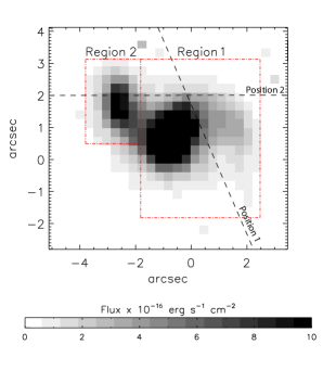
Figure 3: UM 420: H$\alpha$ emission per 0.33$\times$0.33 arcsec² spaxel. The two main areas of H$\alpha$ emission have been used to define two main star-forming regions. Also overlaid on the map are the locations of position-velocity cuts used for the P-V diagrams shown in Figure 4.

A FWHM map for H$\alpha$ is shown in the right-hand panel of Figure 2(a). The highest measured FWHM is $\sim$270 km s^-1, located southwards of the central emission peak, along the southern edge of the galaxy. The central flux peak is aligned with a peak of $\sim$160 km s^-1 whereas the second, easterly, flux peak is located within an area of decreased FWHM, $\sim$130 km s^-1, surrounded by a slightly higher FWHM area of $\sim$150 km s^-1. The south-western arm harbours the lowest line FWHM of $\sim$80–120 km s^-1.

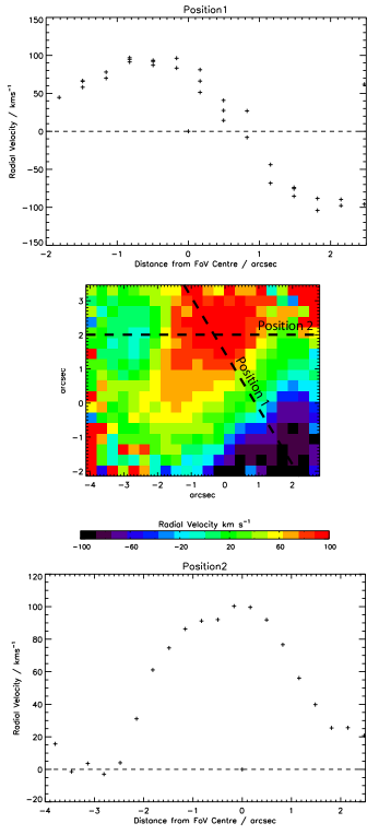
Figure 4: Position velocity (P-V) diagrams for UM 420 in H$\alpha$: central panel: radial velocity map of UM 420 (see Figure 2(a) for details) where the black dotted line overlaid on the map represents cuts orthogonal to the two proposed axes of rotation, as used for the P-V diagrams in the top and bottom panels; top panel: P-V diagram for H$\alpha$ along Position 1, defined as 50^∘ east of north; bottom-panel: P-V diagram for H$\alpha$ along Position 2, at 110^∘ east of north. Zero-point velocities are relative to a recession velocity of $+$17,514 km s^-1. Typical relative radial velocity errors are estimated as 30 km s^-1, with an estimated spatial uncertainty of 0.5 spaxels ($\pm$0.17^′′).

3.2.2 UM 462

UM 462 exhibits a far more disrupted morphology than UM 420. The left-hand panel of Figure 2(b) shows a peak in H$\alpha$ flux located at $\alpha=11^{\rm h}\,53^{\rm m}\,20.25\pm 0.1^{\rm s}$, $\delta=-02^{\circ}\,32^{\prime}\,19.62\pm 0.1^{\prime\prime}$ (J2000), with a surface brightness of 5.34$\times$10^-14 erg cm^-2 s^-1 arcsec^-2. Three additional flux peaks can be seen, located 2.5^′′ northeast, 3.05^′′ east and 8.9^′′ east of this central peak. These H$\alpha$ peaks provide the basis for defining four main star-forming regions, as displayed in Figure 5. Three of the regions have a similar peak surface brightness of 2.0–2.4$\times$10^-13 erg cm^-2 s^-1 arcsec^-2. Region 4 lies farthest away from the brightest SF region (Region 1), at almost 9^′′; a large low surface brightness envelope ($\sim$5$\times$10^-14 erg cm^-2 s^-1 arcsec^-2) separates it from Regions 1–3. It could be the result of interaction with the nearby galaxy UM 461 (Taylor:1995). Previous $R$-band and H i imaging by Taylor:1995 and VRI surface photometry by Telles:1995thesis revealed only two star-forming regions within UM 462 which correspond to Regions 1 and 2 in Figure 5. The H$\alpha$ flux measured by IT98 amounts to 35% of the corresponding VIMOS IFU flux, in accordance with the fraction of the galaxy’s emitting area intercepted by IT98’s slit. The radial velocity distribution of H$\alpha$, displayed in the central panel of Figure 2(b), shows no overall velocity structure through the galaxy. UM 462, being part of an interacting binary pair of galaxies, has a highly disturbed velocity distribution which shows no spatial correlation with flux (Figure 2(b): left-hand panel). The brightest region (Region 1) has a radial velocity of $\sim$0–10 km s^-1, as does the majority of the emitting gas. The largest radial velocity lies directly south-east of this region, with a magnitude of $+$50 km s^-1, in an area of low surface brightness emission. This velocity space extends into the envelope separating Region 4 from Regions 1–3. Region 4 itself lies within a space of negative radial velocity, where again the peaks in velocity and flux are spatially uncorrelated.

The H$\alpha$ FWHM map of UM 462 (right-hand panel of Figure 2(b)) shows no spatial correlation with the flux distribution and only a minimal correlation with radial velocity (Figure 2(b):central panel). A peak in the FWHM of H$\alpha$ is seen $\sim$1^′′ south of the emission peak of Region 4, at 130 km s^-1, which aligns with the negative radial velocity peak.

3.3 [O iii] and [N ii]

Emission line maps of both galaxies in the light of [O iii] $\lambda$5007 and [N ii] $\lambda$6584 lines are shown in Figs  6 and 7. For UM 420 the morphology of [O iii] is similar to that of H$\alpha$ exhibiting two main starbursting regions along with the arc-like ‘arm’ protruding from the brighter region. In UM 462, which is the nearest of the two objects, the [O iii] map shows more structure that the corresponding H$\alpha$ map with an additional area of compact emission to the south-west of Region 1 of Fig  5. According to the morphological criteria of Cairos et al. (2001) these maps support the designation of UM 462 as being of ‘iI,C’ type (irregular; cometary appearance) rather than of ‘iE’ type; UM 420 can be classified as ‘iI, M’ (merging). For both BCGs, the [N ii] morphology is more diffuse and extended that that of [O iii]. The wider distribution of [N ii] is probably due to the effect of lower energy photons surviving farther away from the massive ionising clusters and allowed to produce N⁺ beyond the O²⁺ zone.

Figure 5: UM 462: H$\alpha$ emission per 0.33$\times$0.33 arcsec² spaxel. The four main H$\alpha$ emission areas have been labelled Regions 1–4.

4 Electron Temperature and Density Diagnostics

The dereddened [O iii] ($\lambda$5007 $+$ $\lambda$4959)/$\lambda$4363 intensity ratios were used to determine electron temperatures within each galaxy. The $T_{\rm e}$ values were computed by inputting [O iii] intensity ratios and an adopted electron density into iraf’s TEMDEN task in the NEBULA package. Atomic transition probabilities and collisional strengths for O²⁺ were taken from Wiese:1996 and Lennon:1994, respectively. From the summed spectra over each galaxy (Table LABEL:tab:fluxes) and adopting the electron densities quoted below we derived mean electron temperatures of $\sim$14,000 K and $\sim$13,700 K for UM 420 and UM 462, respectively (Table 4). Using the same method, $T_{\rm e}$ maps were derived using [O iii] ($\lambda$5007 $+$ $\lambda$4959)/$\lambda$4363 emission map ratios. Average $T_{\rm e}$ values for the regions corresponding to peaks in H$\alpha$ emission for UM 420 and UM 462 are given in Tables 6 and 8, respectively, using the regionally integrated relative line intensities (Tables 5, 7). The $T_{\rm e}$ values from the summed spectra were adopted when computing $N_{\rm e}$ values from the [S ii] doublet ratio $\lambda$6717/$\lambda$6731: we derived average $N_{\rm e}$ values of $\sim$170 cm^-3 and $\sim$90 cm^-3 for UM 420 and UM 462, respectively (Table 4). Similarly, the $T_{\rm e}$ maps were used to compute $N_{\rm e}$ maps from $\lambda$6717/$\lambda$6731 ratio maps, which were then adopted for the computation of ionic abundance maps discussed in the following Section. Average $N_{\rm e}$ values for the regions corresponding to peaks in H$\alpha$ emission for UM 420 and UM 462 are given in Tables 6 and 8, respectively.

5 Chemical Abundances

Figure 6: UM 420: The distribution of flux per 0.33$\times$0.33 arsec² spaxels of [O iii] $\lambda$5007 (left panel) and [N ii] $\lambda$6584 (right panel)

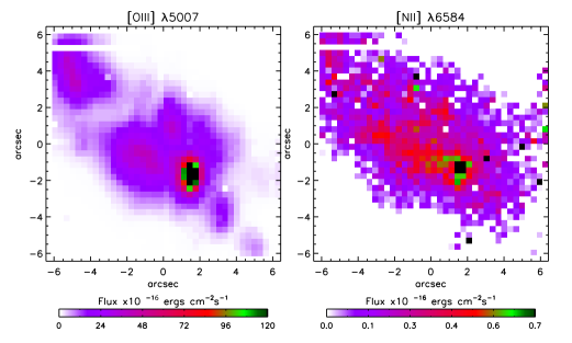
Figure 7: UM 462: The distribution of flux per 0.33$\times$0.33 arsec² spaxels of [O iii] $\lambda$5007 (left panel) and [N ii] $\lambda$6584 (right panel)

Table 4: Ionic and elemental abundances for UM 420 and UM 462 derived, from summed IFU spectra over each galaxy. All ionisation correction factors (ICFs) are taken from Kingsburgh & Barlow, (1994).

Property	UM 420	UM 462
Te (O III)/ K	14000$\pm$ 1500	13700$\pm$ 350
Ne (S II)/ cm-3	170$\pm$ 80	90$\pm$ 75
c(H$\beta$)	0.25$\pm$0.08	0.19$\pm$0.04
He+/H+ ($\lambda$4471) $\times 10^{2}$	7.65$\pm$1.03	6.68 $\pm$0.62
He+/H+ ($\lambda$5876) $\times 10^{2}$	9.07$\pm$0.54	8.63 $\pm$0.71
He+/H+ ($\lambda$6678) $\times 10^{2}$	10.6$\pm$3.6	10.4 $\pm$ 0.72
He+/H+ mean $\times 10^{2}$	9.09$\pm$1.20	8.58 $\pm$0.72
He2+/H+ ($\lambda$4686)$\times 10^{3}$	—	1.45 $\pm$ 0.08
He/H $\times 10^{2}$	9.09$\pm$1.20	8.73 $\pm$0.72
O+/H+a $\times 10^{5}$	5.51$\pm^{3.35}_{1.56}$	4.32$\pm^{0.43}_{0.36}$
O++/H+ $\times 10^{5}$	5.24$\pm^{1.96}_{1.13}$	6.30$\pm^{0.50}_{0.44}$
O/H $\times 10^{4}$	1.08$\pm^{0.53}_{0.27}$	1.06$\pm^{0.09}_{0.08}$
12+log(O/H)	8.03$\pm^{0.17}_{0.13}$	8.03$\pm^{0.04}_{0.07}$
N+/H+ $\times 10^{6}$	1.94$\pm^{0.68}_{0.44}$	0.61$\pm^{0.05}_{0.05}$
ICF(N)	1.95$\pm^{2.12}_{1.04}$	2.46$\pm^{0.46}_{0.39}$
N/H $\times 10^{6}$	3.79$\pm^{6.86}_{2.42}$	1.50$\pm^{0.43}_{0.33}$
12+log(N/H)	6.58$\pm^{0.45}_{0.44}$	6.18$\pm^{0.11}_{0.11}$
log(N/O)	$-$1.45$\pm^{0.57}_{0.62}$	$-$1.85$\pm^{0.14}_{0.15}$
Ne++/H+ $\times 10^{5}$	3.33$\pm^{2.24}_{1.09}$	—
ICF(Ne)	2.05$\pm^{1.86}_{0.93}$	—
Ne/H $\times 10^{5}$	6.84$\pm^{14.98}_{4.33}$	—
12+log(Ne/H)	7.83$\pm^{0.50}_{0.43}$	—
log(Ne/O)	$-$0.20$\pm^{0.63}_{0.61}$	—
S+/H+ $\times 10^{7}$	5.58$\pm^{1.66}_{1.12}$	3.30$\pm^{0.33}_{0.30}$
S++/H+ $\times 10^{6}$	2.55${}^{b}\pm^{1.84}_{0.85}$	1.20$\pm^{0.34}_{0.29}$
ICF(S)	0.81$\pm^{0.19}_{0.49}$	0.62$\pm^{0.14}_{0.13}$
S/H $\times 10^{6}$	2.53$\pm^{2.58}_{1.84}$	0.96$\pm^{0.51}_{0.35}$
12+log(S/H)	6.40$\pm^{0.31}_{0.56}$	5.98$\pm^{0.18}_{0.20}$
log(S/O)	$-$1.63$\pm^{0.43}_{0.74}$	$-$2.05$\pm^{0.22}_{0.24}$
Ar++/H+ $\times 10^{7}$	—	3.71$\pm^{0.19}_{0.17}$s
ICF(Ar)	—	1.07$\pm^{0.05}_{0.03}$
Ar/H $\times 10^{7}$	—	3.98$\pm^{0.38}_{0.31}$
log(Ar/O)	—	$-$2.43$\pm^{0.08}_{0.07}$

^a

Derived using [O II] $\lambda$3727 flux from IT98

^b

Derived using the relationship between S²⁺ and S⁺ (Equation A38) of Kinsgburgh & Barlow (1994)

Abundance maps relative to H⁺ were created for the N⁺, O²⁺, S⁺ and S²⁺ ions, using the $\lambda\lambda$6584, 5007, 6717$+$6731 and 6312 lines, respectively, when the appropriate line was detected. Examples of flux maps used in the derivations of these abundance maps can be seen in Figures 6 and 7, showing the distribution of flux in the [O iii] $\lambda$5007 and [N ii] $\lambda$6584 emission lines for UM 420 and UM 462, respectively. Since the [S iii] $\lambda$6312 line was not detected from UM 420, its S²⁺/H⁺ abundance was estimated using an empirical relationship between the S²⁺ and S⁺ ionic fractions (equation A38) from Kingsburgh:1994. Ionic abundances were calculated using iraf’s IONIC task, using each galaxy’s respective $T_{\rm e}$ and $N_{\rm e}$ maps described above, with each VIMOS spaxel treated as a distinct ‘nebular zone’ with its own set of physical conditions. Ionic abundance ratios were also derived from the summed spectra fluxes, whose $T_{\rm e}$’s and $N_{\rm e}$’s are listed in Table 4, using the program equib06 (originally written by I. D. Howarth and S. Adams). Table 4 also includes a Ne²⁺/H⁺ abundance ratio for UM 420, as the [Ne iii] $\lambda$3969 line was redshifted into the HRblue spectral range, and an Ar²⁺/H⁺ ratio for UM 462. Abundance maps were however not created for either ion due to the low S/N ratio [Ne iii] $\lambda$3969 and [Ar iii] $\lambda$7135 emission line maps, and the N/H and Ar/H listed in Table 4 have been computed from integrated line ratios across the IFU. Differences between abundances derived using the different atomic data tables utilised by IONIC and equib06 were investigated by also using IONIC to compute abundances from the summed spectra. Typical differences were found to be $\sim$2% or less. Since [O ii] $\lambda$3727 is not redshifted into the VIMOS spectral range for either galaxy we have to rely on published fluxes. We therefore adopted $F$($\lambda$3727)/$F$(H$\beta$) values of 2.02$\pm$0.04 and 1.46$\pm$0.01 for UM 420 and UM 462, respectively (from IT98), and corrected them for reddening using the mean $c$(H$\beta$) values derived here (see Table LABEL:tab:fluxes). The spectra of IT98 were obtained using the 2.1-m Kitt Peak Observatory GoldCam spectrograph’s 3${}^{\prime\prime}\times$200^′′ slit aligned to collect the maximum amount of flux from the targets. For UM 420, whose GoldCam and VIMOS H$\alpha$ fluxes agree within 11 per cent, the adoption of [O ii] fluxes from IT98 should introduce only minor uncertainties in our analysis; for UM 462 whose H$\alpha$ flux measured by IT98 is 35% of the VIMOS flux, larger uncertainties might be expected. It is encouraging however that the relative line fluxes and intensities listed in Table LABEL:tab:fluxes differ from those of IT98 by an average factor of only 0.96 for UM 420 and 1.09 for UM 462. Hence for the derivation of the O⁺ abundance we adopted a constant $I$($\lambda$3727)/$I$(H$\beta$) ratio for each galaxy. As a result we cannot, for instance, comment on the spatial variance of the N/O abundance ratio across the galaxies. An alternative method for deriving an O⁺ abundance map was investigated in which global O⁺/N⁺ ratios of 16.49 and 37.64 from IT98 for UM 420 and UM 462, respectively, were multiplied by the corresponding N⁺/H⁺ IFU maps. Overall it was found that maps derived using the ‘global factor’ method yielded elemental oxygen abundances $\sim$40% higher and nitrogen abundances $\sim$55% lower than those derived from a constant $I$($\lambda$3727)/$I$(H$\beta$) ratio for each galaxy. However, by deriving an O⁺ abundance map in this way we would be prevented from creating a meaningful N/H map since ICF(N) $=$ O/O⁺. We therefore opted to use the O⁺ abundance maps derived from the constant $\lambda$3727 fluxes when creating ICF(N), ICF(S) and O/H abundance maps.

Ionic nitrogen, neon and sulphur abundances were converted into N/H, Ne/H and S/H abundances using ionisation correction factors (ICFs) from Kingsburgh:1994. Average abundances from integrated galaxy spectra are listed in Table 4. Elemental O/H abundance maps for UM 420 and UM 462 are shown in Figure 8, while average ionic and elemental abundances derived from spectra summed over each individual star-forming region are listed in Tables 6 and 8 for UM 420 and UM 462, respectively.

5.1 UM 420

Table 5: UM 420 regional fluxes and intensities used for regional T_e and N_e diagnostics and regional ionic abundance calculations.

	Region 1		Region 2
Line ID	F($\lambda$)	I($\lambda$)	F($\lambda$)	I($\lambda$)
4340 H$\gamma$	40.43$\pm$ 0.49	45.05$\pm$ 0.54	32.44$\pm$ 1.15	35.86$\pm$ 1.27
4363 [O iii]	4.51$\pm$ 0.31	5.00$\pm$ 0.35	5.34$\pm$ 0.78	5.88$\pm$ 0.86
4471 He i	4.14$\pm$ 0.33	4.49$\pm$ 0.36	4.92$\pm$ 0.59	5.30$\pm$ 0.64
4861 H$\beta$	100.00$\pm$ 1.04	100.00$\pm$ 1.04	100.00$\pm$ 1.80	100.00$\pm$ 1.80
4959 [O iii]	140.57$\pm$ 1.47	137.72$\pm$ 1.44	168.37$\pm$ 2.69	165.20$\pm$ 2.64
5007 [O iii]	441.01$\pm$ 4.40	427.64$\pm$ 4.27	514.34$\pm$ 8.13	499.91$\pm$ 7.91
5876 He i	13.04$\pm$ 0.31	10.86$\pm$ 0.26	11.29$\pm$ 0.79	9.53$\pm$ 0.67
6563 H$\alpha$	366.84$\pm$ 5.21	278.98$\pm$ 3.96	296.63$\pm$ 3.88	230.33$\pm$ 3.01
6584 [N ii]	29.66$\pm$ 0.31	22.50$\pm$ 0.24	16.80$\pm$ 0.98	13.02$\pm$ 0.76
6678 He i	2.24$\pm$ 0.32	1.68$\pm$ 0.24	—	—
6716 [S ii]	30.15$\pm$ 0.51	22.52$\pm$ 0.38	24.11$\pm$ 0.89	18.40$\pm$ 0.68
6731 [S ii]	23.31$\pm$ 0.51	17.37$\pm$ 0.38	20.81$\pm$ 0.94	15.86$\pm$ 0.72
F(H$\beta$)a	300.4$\pm$ 3.330		48.414$\pm$ 0.874

^a in units of $10^{-16}$erg s^-1 cm^-2

The line fluxes for the summed spectra over Regions 1 and 2 of UM 420 are listed in Table 5 and the average physical properties from which they are derived are listed in Table 6. A graphical representation of the variations in elemental and ionic abundances between Regions 1 and 2 is shown in Figure 9.

Table 6: Ionic and elemental abundances for UM 420, derived from summed IFU spectra over each region. All ionisation correction factors (ICFs) are taken from Kingsburgh & Barlow, (1994).

Property	Region 1	Region 2
Te (O III)/ K	12300$\pm$330	12900$\pm$680
Ne (S II)/ cm-3	120$\pm$55	300$\pm$160
c(H$\beta$)	0.37$\pm$0.04	0.34$\pm$0.08
O+/H+a $\times 10^{4}$	0.95$\pm$ 0.12	0.89$\pm$ 0.25
O++/H+ $\times 10^{4}$	0.79$\pm$ 0.07	0.92$\pm$ 0.18
O/H $\times 10^{4}$	1.74$\pm$ 0.19	1.81$\pm$ 0.43
12+log(O/H)	8.24$\pm$ 0.05	8.26$\pm$ 0.09
N+/H+ $\times 10^{6}$	2.67$\pm$ 0.18	1.55$\pm$ 0.22
N/H $\times 10^{6}$	4.89$\pm$ 1.60	3.15$\pm$ 2.39
12+log(N/H)	6.69$\pm$ 0.12	6.50$\pm$ 0.25
log(N/O)	$-$1.55$\pm$ 0.17	$-$1.76$\pm$ 0.33
S+/H+ $\times 10^{7}$	13.38$\pm$ 0.92	11.26$\pm$ 1.65
S++/H+b $\times 10^{6}$	7.47$\pm$ 0.49	6.39$\pm$ 0.89
S/H $\times 10^{6}$	7.58$\pm$ 1.51	5.87$\pm$ 2.62
12+log(S/H)	6.88$\pm$ 0.08	6.77$\pm$ 0.16
log(S/O)	$-$1.36$\pm$ 0.12	$-$1.49$\pm$ 0.24

^a

Derived using [O II] $\lambda$3727 flux from IT98

^b

Derived using the relationship between S²⁺ and S⁺(Equation A38) of Kinsgburgh & Barlow (1994)

The elemental oxygen abundance map shown in the left-hand panel of Figure 8 displays two peaks whose locations correlate with the two H$\alpha$ peaks of UM 420 (marked in Figure 3). Minimal abundance variations are seen between Regions 1 and 2, whose average metallicity is 12 $+$ log(O/H) $\sim$ 8.25 $\pm$ 0.07. Adopting a solar oxygen abundance of 8.71$\pm$0.10 relative to hydrogen (Scott:2009), this corresponds to an oxygen abundance of $\sim$0.35 solar for Regions 1 and 2. This is $\sim$0.2 dex higher than the value derived from the integrated spectrum of the whole galaxy. This could point to some limited oxygen enrichment in the areas corresponding to the peak H$\alpha$ emission, that is the clusters associated with Regions 1 and 2. However, since all the oxygen abundances overlap within their 1$\sigma$ uncertainties, we cannot conclude that this variation in oxygen abundance is significant. The nitrogen abundances of the two regions of star-formation are consistent within their uncertainties (Table 6 ). The N/O ratios for both regions are consistent with those of other metal-poor emission line galaxies of similar oxygen metallicity (Izotov:2006a), and do not show the nitrogen excess reported by Pustilnik:2004. The S/O ratio for Region 1 is slightly higher than expected for BCGs, although Region 2 is closer to the average reported range of log(S/O) $\sim$ $-$1.4 – $-$1.7 (Izotov:2006a).

5.2 UM 462

Table 7: UM 462 regional fluxes and intensities used for regional T_e and N_e diagnostics and regional ionic abundance calculations.

	Region 1		Region 2		Region 3		Region 4
Line ID	F($\lambda$)	I($\lambda$)	F($\lambda$)	I($\lambda$)	F($\lambda$)	I($\lambda$)	F($\lambda$)	I($\lambda$)
4340 H$\gamma$	40.92$\pm$ 0.72	46.49$\pm$ 0.49	45.97$\pm$ 0.41	43.39$\pm$ 0.54	45.98$\pm$ 0.41	53.86$\pm$ 0.48	43.39$\pm$ 0.54	44.45$\pm$ 0.56
4363 [O iii]	8.61$\pm$ 0.18	9.26$\pm$ 0.19	7.27$\pm$ 0.26	7.55$\pm$ 0.27	9.17$\pm$ 0.70	10.67$\pm$ 0.82	6.62$\pm$ 0.53	6.77$\pm$ 0.55
4471 He i	3.01$\pm$ 0.14	3.19$\pm$ 0.15	3.51$\pm$ 0.16	3.61$\pm$ 0.16	3.66$\pm$ 0.34	4.12$\pm$ 0.38	3.63$\pm$ 0.40	3.70$\pm$ 0.40
4686 He ii	—	—	1.21$\pm$ 0.12	1.22$\pm$ 0.12	—	—	—	—
4861 H$\beta$	100.00$\pm$ 0.65	100.00$\pm$ 0.65	100.00$\pm$ 0.65	100.00$\pm$ 0.65	100.00$\pm$ 0.65	100.00$\pm$ 0.65	100.00$\pm$ 0.76	100.00$\pm$ 0.76
4959 [O iii]	218.90$\pm$ 1.90	215.76$\pm$ 1.87	169.17$\pm$ 1.30	167.95$\pm$ 1.29	182.95$\pm$ 1.23	177.54$\pm$ 1.19	174.63$\pm$ 1.52	173.83$\pm$ 1.51
5007 [O iii]	630.70$\pm$ 5.95	617.18$\pm$ 5.82	503.02$\pm$ 2.64	497.58$\pm$ 2.61	564.84$\pm$ 2.32	539.98$\pm$ 2.22	507.96$\pm$ 4.43	504.49$\pm$ 4.40
5876 He i	14.47$\pm$ 0.16	12.72$\pm$ 0.14	9.77$\pm$ 0.59	9.16$\pm$ 0.55	15.02$\pm$ 0.64	11.48$\pm$ 0.49	—	—
6563 H$\alpha$	332.75$\pm$ 0.98	274.41$\pm$ 0.81	325.84$\pm$ 2.44	295.81$\pm$ 2.22	483.79$\pm$ 3.16	324.20$\pm$ 2.12	293.19$\pm$ 4.92	275.84$\pm$ 4.63
6584 [N ii]	4.25$\pm$ 0.11	3.50$\pm$ 0.09	6.88$\pm$ 0.23	6.24$\pm$ 0.21	9.88$\pm$ 0.48	6.60$\pm$ 0.32	5.04$\pm$ 0.42	4.74$\pm$ 0.40
6678 He i	2.34$\pm$ 0.10	1.91$\pm$ 0.08	3.21$\pm$ 0.13	2.90$\pm$ 0.12	5.19$\pm$ 0.44	3.41$\pm$ 0.29	—	—
6716 [S ii]	7.53$\pm$ 0.10	6.13$\pm$ 0.08	16.11$\pm$ 0.20	14.53$\pm$ 0.18	28.09$\pm$ 0.72	18.32$\pm$ 0.47	11.99$\pm$ 0.38	11.23$\pm$ 0.35
6731 [S ii]	5.56$\pm$ 0.10	4.52$\pm$ 0.08	11.91$\pm$ 0.20	10.74$\pm$ 0.18	19.90$\pm$ 0.73	12.95$\pm$ 0.47	8.79$\pm$ 0.40	8.23$\pm$ 0.37
F(H$\beta$)a	1065.01$\pm$ 6.32		594.32$\pm$6.03		96.24$\pm$2.33		275.04$\pm$ 15.62

^a in units of $10^{-16}$erg s^-1 cm^-2

Table 7 lists the fluxes from summed spectra over Regions 1–4 of UM 462. The average ionic and elemental abundances, along with the average $T_{\rm e}$ and $N_{\rm e}$ values, derived from the summed spectra over the respective regions are listed in Table 8. A graphical representation of the variation in elemental and ionic abundances across Regions 1–4 is shown in Figure 9.

Table 8: Ionic and elemental abundances for UM 462, derived from summed IFU spectra over each region. All ionisation correction factors (ICFs) are taken from Kingsburgh & Barlow, (1994).

Property	Region 1	Region 2	Region 3	Region 4
Te (O III)/ K	13400$\pm$150	13500$\pm$230	15200$\pm$500	12800$\pm$440
Ne (S II)/ cm-3	70$\pm$40	70 $\pm$40	20$\pm^{70}_{10}$	60$\pm$50
c(H$\beta$)	0.26$\pm$0.03	0.13$\pm$0.03	0.54$\pm$0.03	0.08$\pm$0.08
O+/H+a $\times 10^{5}$	4.85$\pm$ 0.28	4.38$\pm$ 0.33	3.91$\pm$ 0.44	5.09$\pm$ 0.81
O++/H+ $\times 10^{5}$	8.86$\pm$ 0.30	6.99$\pm$ 0.34	5.58$\pm$ 0.49	8.17$\pm$ 0.88
O/H $\times 10^{4}$	1.37$\pm$ 0.06	1.14$\pm$ 0.07	0.95$\pm$ 0.09	1.33$\pm$ 1.49
12+log(O/H)	8.14$\pm$ 0.02	8.06$\pm$ 0.02	7.98$\pm$ 0.04	8.12$\pm$ 0.05
N+/H+$\times 10^{6}$	0.34$\pm$ 0.01	0.60$\pm$ 0.02	0.50$\pm$ 0.03	0.51$\pm$ 0.04
N/H $\times 10^{6}$	0.97$\pm$ 0.13	1.56$\pm$ 0.28	1.22$\pm$ 0.41	1.33$\pm$ 0.56
12+log(N/H)	5.99$\pm$ 0.05	6.19$\pm$ 0.07	6.08$\pm$ 0.13	6.12$\pm$ 0.15
log(N/O)	$-$2.15$\pm$ 0.07	$-$1.86$\pm$ 0.10	$-$1.89$\pm$ 0.17	$-$2.00$\pm$ 0.21
S+/H+ $\times 10^{7}$	3.01$\pm$ 0.09	7.04$\pm$ 0.28	7.06$\pm$ 0.45	6.01$\pm$ 0.51
S++/H+ $\times 10^{6}$	0.96$\pm$ 0.04	1.27$\pm$ 0.08	1.37$\pm$ 0.15	1.97$\pm$ 0.26
S/H $\times 10^{6}$	0.66$\pm$ 0.12	1.15$\pm$ 0.27	1.32$\pm$ 0.51	1.49$\pm$ 0.80
12+log(S/H)	5.82$\pm$ 0.07	6.06$\pm$ 0.09	6.12$\pm$ 0.14	6.17$\pm$ 0.19
log(S/O)	$-$2.32$\pm$ 0.09	$-$2.00$\pm$ 0.12	$-$1.86$\pm$ 0.19	$-$1.95$\pm$ 0.24

^a

Derived using [O II] $\lambda$3727 flux from IT98

The right-hand panel of Figure 8(a) shows the O/H abundance ratio map for UM 462. The oxygen abundance varies spatially across the different star-forming regions of UM 462 (as marked in Figure 5). Four maxima in oxygen abundance are seen across the map, all aligning spatially with peaks in H$\alpha$ emission (shown as overlaid contours), with the exception of Region 1, where the maximum in oxygen abundance appears to lie $\sim$1.5^′′ south of the H$\alpha$ peak of Region 1. A decrease in the oxygen abundance can be seen $\sim$1.0^′′ north-east of the peak in Region 1. Oxygen abundances for Regions 1–4 are listed in Table 8. A maximum variation of 40% is seen between Region 1 (displaying the highest metallicity) and Region 3 (displaying the lowest). The mean oxygen abundance of the four identified star-forming regions in UM 462 is 12 $+$ log(O/H) $=$ 8.08 $\pm$ 0.94, that is, $\sim$0.25 solar. This is in good agreement with the value derived from the integrated spectrum of the whole galaxy. Regional N/H and S/H abundance ratios are given in Table 8. Regions 2, 3 and 4 have the same nitrogen abundance within the uncertainties. The maximum difference (0.2 dex) is between Regions 2 and 1; the latter shows the lowest nitrogen abundance. In comparison with metal-poor emission line galaxies of similar metallicity (Izotov:2006a), UM 462 appears to be overall slightly nitrogen poor. The sulphur abundance across the galaxy is variable with Region 1 having the lowest, a factor of $\sim$ 2 below the other three regions. In comparison with other emission line galaxies, UM 462 displays a lower than average log(S/O) of $-$2.03 [typical values range from $\sim$ $-$1.4 to $-$1.7; Izotov:2006a].

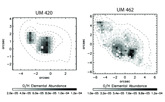
Figure 8: O/H abundance ratio maps of UM 420 (left panel) and UM 462 (right panel) derived from their respective O²⁺ and O⁺ ionic abundance maps and $T_{\rm e}$ and $N_{\rm e}$ maps, as described in Section 5. Overlaid are the H$\alpha$ flux contours from Figure 2(a).

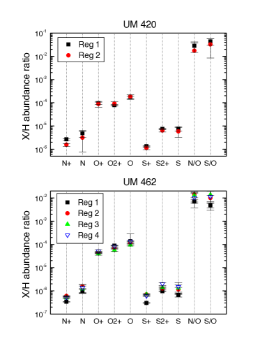
Figure 9: Graphical representation of the variations in ionic and elemental abundances across UM 420 and UM 462, as given in Tables 6 and 8, respectively.

5.2.1 Helium abundances

Following the method outlined by Tsamis:2003 and Wesson:2008, abundances for helium were derived using atomic data from Smits:1996, accounting for the effects of collisional excitation using the formulae in Benjamin:1999. Ionic and total helium abundances relative to hydrogen derived from helium recombination lines measured from summed spectra over the entire galaxies are given in Table 4 (derived using the global $T_{\rm e}$ and $N_{\rm e}$ values from the same Table). Given that the reddening varies across the galaxies (predominantly in the case of UM 462), and in order to minimise the uncertainties, we have also computed helium abundances per each individual star forming region; these are given in Tables LABEL:tab:HeAbundsum420 and LABEL:tab:HeAbundsum462, for UM 420 and UM 462, respectively. These values are derived from summed spectra over each star-forming region of the galaxy dereddened with the corresponding $c$(H$\beta$). Our adopted mean values for He⁺/H⁺ were derived from the $\lambda$4471, $\lambda$5876 and $\lambda$6678 lines, averaged with weights 1:3:1. The helium abundances were calculated for the average temperatures and densities given in Tables 6 and 8. Regional helium abundances were not calculated for Region 4 of UM 462 because only one He i line was detected (see Table 7). Helium abundances derived from summed spectra are found to agree with those derived in IT98, within the uncertainties.

Table 9: Ionic and elemental helium abundances for UM 420 derived from summed spectra over each region.^a

	Region 1	Region 2
He+/H+ ($\lambda$4471) $\times 10^{2}$	9.23$\pm$0.73	10.77$\pm$1.23
He+/H+ ($\lambda$5876) $\times 10^{2}$	8.31$\pm$0.20	7.15$\pm$0.52
He+/H+ ($\lambda$6678) $\times 10^{2}$	4.56$\pm$0.66 :	—
He+/H+ mean $\times 10^{2}$	8.54$\pm$0.33	8.05$\pm$0.70
He2+/H+ ($\lambda$4686)$\times 10^{3}$	—	—
He/H $\times 10^{2}$	8.54$\pm$0.33	8.05$\pm$0.70

^a

Entries followed by ‘:’ were excluded from the final average.

Table 10: Ionic and elemental helium abundances for UM 462 derived from summed spectra over each Region (with the exclusion of Region 4, where only one He i line was detected).^a

	Region 1	Region 2	Region 3
He+/H+ ($\lambda$4471) $\times 10^{2}$	6.66$\pm$0.32	7.54$\pm$0.34	8.75$\pm$0.81
He+/H+ ($\lambda$5876) $\times 10^{2}$	9.97$\pm$0.10	7.20$\pm$0.43	9.33$\pm$ 0.40
He+/H+ ($\lambda$6678) $\times 10^{2}$	5.34$\pm$0.23 :	8.11$\pm$ 0.33	9.83$\pm$0.84
He+/H+ mean $\times 10^{2}$	9.14$\pm$0.16	7.45$\pm$0.39	9.31$\pm$0.57
He2+/H+ ($\lambda$4686)$\times 10^{3}$	—	1.04$\pm$0.11	—
He/H $\times 10^{2}$	9.14$\pm$0.16	7.55$\pm$0.40	9.31$\pm$0.57

^a

Entries followed by ‘:’ were excluded from the final average.

5.3 Stellar Properties

5.3.1 Wolf-Rayet features?

Contrary to previous long slit studies (Izotov:1998; Schaerer:1999; Guseva:2000), which had limited spatial coverage, the VIMOS IFU spectra do not reveal any evidence for broad WR emission features at either $\sim$4686 Å or at $\sim$5808, 5812 Å. This is true for single spaxel spectra, summed spectra over Region 1 (the highest surface brightness SF region in both galaxies) or in the summed spectra over the whole of each galaxy, as shown in Figure 10. Hence this analysis does not support the classification of UM 420 and UM 462 as Wolf-Rayet galaxies. When searching for WR features one must consider the width of the extraction aperture, which can sometimes be too large and thus dilute weak WR features by the continuum flux (Lopez-Sanchez:2008). We therefore also examined the summed spectra over each individual star-forming region, with extraction apertures equal to those displayed in Figures 3 and  5 aiming to reduce the dilution of any WR features. However, those remained undetected. This supports the statement by Schaerer:1999 regarding the dependence of a object’s classification as a ‘WR galaxy’ on the quality of the spectrum, and location and size of the aperture. Given that our spectroscopy was obtained with an 8.2 m telescope, with exposure times of $\sim$1500 s for each spectral region, we conclude that the presence of WR stars in UM 420 and UM 462 is not yet proven.

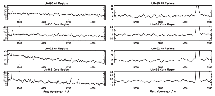
Figure 10: Sections of VIMOS IFU spectra, in flux units of $\times 10^{-16}$ erg s^-1 cm^-2, where the WR ‘blue bump’ feature (left column) and C iv ‘red’ feature (right column) would be located within summed spectra over the core region (labelled Region 1 in Figures 3 and 5 for UM 420 and UM 462, respectively) and over the entire galaxy. There are no detections of WR emission features in any of the spectra.

5.3.2 Starburst ages and star formation rates

Luminosities of hydrogen recombination lines, particularly H$\beta$, can provide estimates of the ionising flux present, assuming a radiation-bounded nebula (Schaerer:1998). Thus, the equivalent width ($EW$) of H$\beta$ is commonly used as an age indicator of the ionising stellar population at a given metallicity. Maps of $EW$(H$\beta$) for UM 420 and UM 462 can be seen in Figure 11(a) & (b), respectively. We can use these maps, in conjunction with the metallicity maps described in Section 5, to estimate the age of the latest star forming episodes throughout UM 420 and UM 462 by comparing the regional observed average $EW$(H$\beta$) values with those predicted by the spectral synthesis code STARBURST99 (Leitherer:1999). For the models we chose metallicities of 0.4 and 0.2 Z_⊙, representative of the average metallicities of UM 420 and UM 462 (derived from regional summed spectra), together with assumptions of an instantaneous burst with a Salpeter initial mass function (IMF), a total mass of 1$\times 10^{6}$ M_⊙ (the default mass chosen by Leitherer:1999 to produce properties that are typical for actual star-forming galaxies), and a 100M_⊙ upper stellar mass limit (which approximates the classical Salpeter:1955 IMF). Models were run for Geneva tracks with “high” mass loss rates (tracks recommended by the Geneva group) and Padova tracks with thermally pulsing AGB stars included. For each of these evolutionary tracks, two types of model atmosphere were used; firstly the Pauldrach-Hillier (PH, the recommended atmosphere) and secondly Lejeune-Schmutz (LS). The latter was chosen because it incorporates stars with strong winds, which would be representative of the WR population within each galaxy (if present). The stellar ages predicted by each model and the observed average $EW$(H$\beta$) within each peak emission region in UM 420 and UM 462 were derived from Figure 12 and are listed in Table LABEL:tab:EWs. The difference between the ages predicted by the Geneva and Padova stellar evolutionary tracks is relatively small, with the Geneva tracks predicting lower ages by up to 20%. The difference in ages predicted by the PH and LS atmospheres are smaller still, with LS predicting lower ages by $\sim$6%. We cannot comment on which atmosphere model is more appropriate given that the existence of WR stars within each galaxy is questioned by the current study, hence we adopt average stellar ages from the four model combinations. The current (instantaneous) star formation rates (SFRs) based on the H$\alpha$ luminosities were calculated following Kennicutt:1998 and are given in Table LABEL:tab:EWs. SFRs corrected for the sub-solar metallicities of these targets are also given, derived following the methods outlined in Lee:2002.

Table 11: Age of the latest star formation episode and current star formation rates.

	Starburst ages (Myr)
	UM 420		UM 462
Model	Reg. 1	Reg. 2	Reg. 1	Reg. 2	Reg. 3	Reg. 4
Padova-AGB PH	4.51$\pm$0.21	5.26$\pm$0.19	4.85$\pm$0.32	5.45$\pm$0.13	5.85$\pm$0.13	5.90$\pm$0.27
Padova-AGB LS	4.24$\pm$0.34	5.16$\pm$0.19	4.66$\pm$0.36	5.31$\pm$0.10	5.66$\pm$0.07	5.76$\pm$0.24
Geneva-High PH	3.76$\pm$0.36	4.91$\pm$0.27	3.91$\pm$0.56	4.86$\pm$0.13	5.21$\pm$0.10	5.51$\pm$0.39
Geneva-High LS	3.50$\pm$0.34	4.71$\pm$0.22	3.76$\pm$0.48	4.61$\pm$0.10	5.01$\pm$0.10	5.21$\pm$0.33
	Star formation rates (M⊙ yr-1)
	UM 420		UM 462
SFR(H$\alpha$)a	10.5	1.31	0.104	0.047	0.021	0.018
SFR(H$\alpha$)b	7.0	0.87	0.069	0.027	0.012	0.013

^a

Derived using the relationship between SFR and $L$(H$\alpha$) from Kennicutt:1998.

^b

Corrected for sub-solar metallicities following Lee:2002.

UM 420: Regions 1 and 2 contain ionising stellar populations with weighted average ages of 3.94$\pm$0.31 and 4.99$\pm$0.21 Myr, respectively (Table LABEL:tab:EWs). Interestingly, the ages returned by all 4 models consistently show Region 2 to be older than Region 1, which could imply that these were in fact once isolated bodies, and that star formation within Region 1 was triggered or is still a product of an ongoing merger with Region 2. This also agrees well with the in-falling merger scenario derived from radial-velocity maps (discussed in Section 3.2.1). However, the significance of the derived difference in ages between the two regions is only at the 2$\sigma$ level. Also in support of this are their respective SFRs which differ by almost an order of magnitude. Global SFRs derived by Lopez-Sanchez:2008 are 3.7 $\pm$ 0.2 M_⊙ yr^-1 (based on an H$\alpha$ flux estimated from broad-band photometry) and 1.9 $\pm$ 0.9 M_⊙ yr^-1 (based on the 1.4 GHz flux), and are lower than our measurements which are based on the monochromatic H$\alpha$ flux.

UM 462: Table LABEL:tab:EWs show average stellar population ages of 4.19$\pm$0.42, 5.07$\pm$0.11, 5.45$\pm$0.10 and 5.56$\pm$0.31 Myr for Regions 1–4, respectively. Since Region 1 shows the highest ionising flux, we would expect it to contain the youngest stellar population. It is notable that the age of the stellar population increases through Regions 2–4 as the distance of separation from Region 1 increases and at the same time the SFR decreases. Our SFRs are comparable to previously published values of 0.13 (based on FIR fluxes), 0.00081 (blue) and 0.5 M_⊙ yr^-1 (narrow-band H$\alpha$) from Sage:1992 and 0.36 (60 $\mu$m) and 0.13 M_⊙ yr^-1 (1.4 GHz) from Hopkins:2002. Evidence suggests that Regions 1–3 are linked in their SF properties, with decreasing metallicity and SFR and increasing stellar population ages as the distance from Region 1 increases. Region 4 breaks this pattern in metallicity harbouring a starburst which is coeval with that of Region 3.

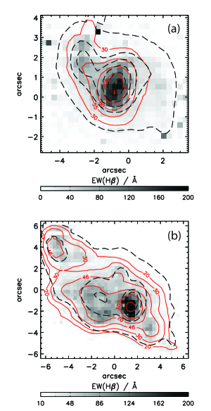
Figure 11: Maps of the equivalent width of H$\beta$ across: (a) UM 420; (b) UM 462. Overlaid red solid lines are contours of $EW$(H$\beta$); black-dashed lines are H$\alpha$ flux contours from Figure 2.

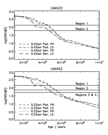
Figure 12: $EW$(H$\beta$) as a function of age, as predicted by the STARBURST99 code for metallicities of 0.4Z_⊙ (UM 420) and 0.2Z_⊙ (UM 462) using a combination of Geneva or Padova stellar evolutionary tracks and Lejeune-Schmutz (LS) or Pauldrach-Hillier (PH) model atmospheres. The observed average $EW$(H$\beta$)’s for each star forming region in UM 420 (top panel) and UM 462 (bottom panel) are overlaid (solid line).

6 Emission Line Galaxy Classification

It is useful to attempt to diagnose the emission line excitation mechanisms in BCGs using the classic diagnostic diagrams of Baldwin:1981 (the BPT diagrams). These are used to classify galaxies according to the dominant excitation mechanism of their emission lines, i.e. either photoionisation by massive stars within H ii regions or photoionisation by non-thermal continua from AGN. The diagrams consist of excitation-dependent and extinction-independent line ratios: log([O iii] $\lambda$5007/H$\beta$) versus either log([S ii] $\lambda$6716 $+$ $\lambda$6731)/H$\alpha$) or log([N ii] $\lambda$6584/H$\alpha$). Star-forming galaxies fall into the lower left region of the diagrams, AGN host galaxies fall into the upper right region and Low-Ionisation Emission Line Regions (LINERs) fall on the lower right. Here we adopt the ‘maximum starburst line’ derived by Kewley:2001 from starburst grids defined by two parameters; metallicities $Z$ = $\sim$ 0.05–3.0 Z_⊙ and ionization parameters $q=5\times 10^{6}$ – $3\times 10^{8}$ cm s^-1, where $q$ is the maximum velocity of an ionisation front that can be driven by the local radiation field and is related to the non-dimensional ionisation parameter $U=q/c$, (Dopita:2001). This line defines the maximum flux ratio an object can have to be successfully fitted by photoionization models alone. Ratios lying above this boundary are inferred to require additional sources of excitation, such as shocks or AGNs. It is thus instructive to see what area of the BPT diagram UM 420 and UM 462 occupy as a whole, as well as their resolved star-forming regions which were defined in Figures 3 and 5.

UM 420: Figure 13(a) and (b) shows the BPT diagram locations of the two star-forming regions within UM 420. Although a large spread can be seen for both regions, Region 2 occupies the higher end of the [O iii] $\lambda$5007/H$\beta$ emission line ratio in both diagrams, and does not exceed the [O iii] $\lambda$5007/H$\beta$ values of Region 1. Some spaxels do cross the ‘maximum starburst line’, but are insufficient in frequency to be considered as evidence for substantial non-thermal line excitation. The [S ii]/H$\alpha$ ratios are generally lower than those predicted by standard predictions of shock models from the literature. There is a larger spread in [N ii] $\lambda$6584/H$\alpha$ as compared to [S ii]/H$\alpha$ which is probably due to the fact that the N⁺/H⁺ abundance ratio differential between Regions 1 and 2 is larger than the corresponding S⁺/H⁺ differential by 45 per cent. In relation to the grid of ($Z$, $q$) models of Kewley:2001, UM 420 lies within a range of $Z=$ 0.4–0.5 Z_⊙and $q\geq 3\times 10^{8}$. This is consistent with the average metallicity of 0.35 $\pm$ 0.06 Z_⊙ for Regions 1 and 2 (Table 6). We conclude that photoionisation by stellar populations is the dominant line excitation mechanism within UM 420.

UM 462: The BPT diagnostic diagrams shown in Figure 14(a) and (b) show the emission line ratios for each spaxel within the four star-forming regions of UM 462 (as defined in Figure 5). As with UM 420 the [S ii]/H$\alpha$ diagnostic ratios tend to straddle the theoretical upper limit for photoionisation. Although their locations appear highly clustered, a slight distinction can be seen for Region 4 which lies slightly to the left of the diagram. The large spread in values can be seen more clearly in Figure 14(b), where the spread along the $X$-axis, i.e. [N ii] $\lambda$6584/H$\alpha$, extends on either side of the other three regions. This range in [N ii] and [S ii] excitation conditions is perhaps to be expected given the 9^′′ distance separating Region 4 from the central regions. Several spaxels’ emission line ratios do spread into the locus of non-thermal excitation but their low occurrence renders them insignificant. In relation to the models of Kewley:2001, UM 462 lies within a range of $Z=$0.2–0.5 Z_⊙and $q\geq 1.5\times 10^{8}$. This is consistent with the average metallicity of $\sim$0.24Z_⊙ for Regions 1–4 (Table 8). We conclude that photoionisation from stellar sources is the dominant excitation mechanism within UM 462 as well. Comparing the two galaxies, the data points of UM 462 are more highly clustered than those of UM 420, despite the former system’s disrupted morphology and are further to the left (smaller values) on the $X$-axis of both diagrams. The explanation probably lies in the higher S/H and N/H abundances of UM 420 compared to those of UM 462 (by corresponding factors of $\sim$ 2.5). Both galaxies display a similar level of [O iii] $\lambda$5007/H$\beta$ excitation.

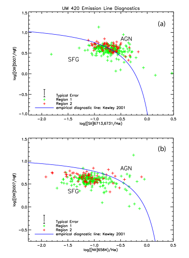
Figure 13: Emission line diagnostic diagrams for UM 420. Each data point represents a spaxel in the ratioed dereddened flux maps corresponding to [O iii] $\lambda$5007/H$\beta$ versus (a) [S ii] $\lambda$6716 $+$ $\lambda$6731/H$\alpha$ and (b) [N ii] $\lambda$6584/H$\alpha$. Spaxels corresponding to the two star-forming regions defined in Figure 3 are separated by colour. The empirical diagnostic ‘maximum starburst’ line from Kewley:2001 is also shown, as are the positions of emission line ratios for star-forming galaxies(SFG) and active galaxies (AGN).

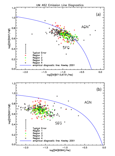
Figure 14: Same as for Figure 13, but for UM 462. Regions 1–4 correspond to the separate star-forming regions defined in Figure 5.

7 Conclusions

We have analyzed VIMOS IFU integral field spectroscopy of the unrelated BCGs UM 420 and UM 462 and studied their morphology by creating monochromatic emission line maps. Both systems show signs of interaction and/or perturbation with the former galaxy currently undergoing a merger (type ‘iI,M’) and the latter displaying a highly disrupted irregular or cometary appearance (type ‘iI,C’; probably due to interaction with a BCG which was not part of this study, UM 461). The spatially resolved emission line maps in the light of [O iii] and H$\alpha$ have revealed two main areas of massive star formation in UM 420 along with an ‘arm-like’ structure, and at least four such areas in UM 462. Current star formation rates were computed from the H$\alpha$ line luminosities for each main starbursting region and the ages of the last major star formation episode were estimated by fitting the observed Balmer line equivalent widths with STARBURST99 models. The two merging components of UM 420 have SFRs that differ by a factor of $\sim$ 8 and starburst episodes separated by 1 Myr. The latest major star formation event took place $\sim$ 4 Myr ago in the largest merging component, and has been producing stars at a rate of 10 M_⊙ yr^-1. In UM 462 the last star forming episode was $\sim$ 4 – 5 Myr ago and has been producing stars at a rate which varies across the galaxy between $\sim$ 0.01 – 0.10 M_⊙ yr^-1, indicative of propagating or triggered star formation.

For both targets the abundances of He, N, O, and S were measured and O/H abundance ratio maps were created based on the direct method of estimating electron temperatures from the [O iii] $\lambda$4363/$\lambda$5007 line ratio. The measured oxygen abundances are 12 $+$ log(O/H) $=$ 8.03 $\pm$ 0.20 for UM 420 and 8.03 $\pm$ 0.10 for UM 462 (20 per cent solar). We find no evidence for significant nitrogen or oxygen variations across the galaxies (at the 0.2 dex level), which would point to self-enrichment from nucleosynthetic products associated with the recent massive star formation activity. Regarding the abundance of nitrogen, and the N/O ratio, this result is in qualitative agreement with the finding that these BCGs cannot be classified as Wolf-Rayet galaxies as the characteristic broad-line stellar features have not been detected by VIMOS; the existence of WR stars in them is an open issue.

8 Acknowledgments

We would like to thank the VIMOS staff at Paranal and Garching for scheduling and taking these service mode observations [programmes 078.B-0353(B, E); PI: Y.G. Tsamis]. We appreciate discussions with Carlo Izzo about the VIMOS instrument and the GASGANO tool. Also, our thanks go to Roger Wesson and Jeremy Walsh for help regarding the derivation of helium abundances. This research made use of the NASA ADS and NED data bases. BLJ acknowledges support from a STFC studentship. YGT acknowledges support from grants AYA2007-67965-C03-02 and CSD2006-00070 CONSOLIDER-2010 “First science with the GTC” of the Spanish Ministry of Science and Innovation.