Supernovae as seen by off-center observers in a local void

Abstract

Inhomogeneous universe models have been proposed as an alternative explanation for the apparent acceleration of the cosmic expansion that does not require dark energy. In the simplest class of inhomogeneous models, we live within a large, spherically symmetric void. Several studies have shown that such a model can be made consistent with many observations, in particular the redshift–luminosity distance relation for type Ia supernovae, provided that the void is of Gpc size and that we live close to the center. Such a scenario challenges the Copernican principle that we do not occupy a special place in the universe. We use the first-year Sloan Digital Sky Survey-II supernova search data set as well as the Constitution supernova data set to put constraints on the observer position in void models, using the fact that off-center observers will observe an anisotropic universe. We first show that a spherically symmetric void can give good fits to the supernova data for an on-center observer, but that the two data sets prefer very different voids. We then continue to show that the observer can be displaced at least fifteen percent of the void scale radius from the center and still give an acceptable fit to the supernova data. When combined with the observed dipole anisotropy of the cosmic microwave background however, we find that the data compells the observer to be located within about one percent of the void scale radius. Based on these results, we conclude that considerable fine-tuning of our position within the void is needed to fit the supernova data, strongly disfavouring the model from a Copernican principle point of view.

Keywords: dark energy theory, supernova type Ia

1 Introduction

The discovery of the dimming of distant type Ia supernovae (SNe Ia) [1, 2] constituted the first impactful evidence that the expansion of the universe is in a phase of acceleration. This picture has been corroborated by several independent probes, including measurements of the cosmic microwave background (CMB) anisotropies [3] and baryon acoustic oscillations (BAO) [4, 5]. Under the assumption that the universe is homogeneous and isotropic, the apparent late-time acceleration is usually attributed to a mysterious energy component with negative pressure – dark energy – the nature of which is still unknown.

In recent years, inhomogeneous universe models of varying degrees of complexity have been the focus of much attention as an alternative explanation of the apparent acceleration that doesn’t require dark energy. The common base in these models is that the assumption of homogeneity and isotropy of the universe is an oversimplification and that it is the presence of inhomogeneities in the distribution of matter that gives rise to the apparent acceleration. Examples of inhomogeneous models include the Swiss-cheese models, which consider light propagation through a universe full of empty regions, and backreaction models, where cosmological perturbation terms are included in the overall dynamics of the universe (see [6] for a review of inhomogeneous models).

In the simplest class of inhomogeneous models, we live within a large, spherically symmetric local void described by the Lemaître-Tolman-Bondi (LTB) metric [7, 8, 9, 10]. The LTB model is an exact solution of Einstein’s equations containing dust only. In contrast to homogeneous universe models, the Hubble expansion rate and the matter density parameter depend on both time and the radial coordinate in LTB models. The apparent acceleration is caused by the radial dependence, such that our local underdense region has a larger Hubble parameter than the surrounding homogeneous universe.

The LTB models violate the Copernican principle by placing the observer in a special place in the universe. Due to the observed near-perfect isotropy of the CMB, the observer is generally assumed to be located very close to the center of the void. Another challenge for the model is that the void must be of Gpc size in order to fit the SN Ia data, but such large voids are extremely improbable in standard models of structure formation [11]. The LTB models thus appear to be unrealistic, but based on observations they have not yet been ruled out. Several studies have shown that with an appropriately chosen void profile, the LTB models can be made to fit data from SNe Ia, CMB and BAO [12, 13, 14, 15, 16, 17, 18, 19]. Further constraints come from considering spectral distortions of the CMB [20] and the kinematic Sunyaev-Zeldovich effect [21].

In the most general scenario, the observer can be located anywhere inside the void, in which case observers living off-center will see an anisotropic universe. There are several ways to test the level of anisotropy in the data to put constraints on the position of an off-center observer. So far, the strongest constraint comes from the dipole anisotropy of the CMB. The observed CMB dipole restricts a static observer to be located within a couple of percent of the void size [22]. The caveat is – although it requires a certain amount of fine-tuning – that a peculiar velocity of the observer directed towards the center can cancel the effect of the off-center position so that large displacements are allowed. For SNe Ia, off-center observers will see an anisotropic relation between the luminosity distance and the redshift. The SN Ia data provide independent constraints on the observer position that complement those imposed by the CMB [23]. Another interesting possibility is to look for cosmic parallax, i.e., a time variation in the angular separation between distant sources induced by the anisotropic expansion. Planned space-based astrometric missions (such as Gaia) could measure the positions of a huge number of quasars over time with outstanding accuracy and thereby establish constraints on the observer position that rival those set by the CMB [24].

This paper deals with the contraints on the observer position coming from SNe Ia. The problem has been addressed previously by Alnes & Amarzguioui [23] who found that it is possible to obtain a better fit to the data for an off-center observer. The constraint on the observer position, however, was found to be fairly weak, partly due to the low number of SNe Ia in the data set employed. Our analysis is similar to theirs, but with a few notable differences. In addition to using new and larger SN Ia data sets as well as a different LTB model, we also investigate whether the model can fit the SNe Ia for an off-center observer while simultaneously accommodate the observed CMB dipole. We find that it is only possible to obtain a good fit to the data as long as the observer is located very close to the void center.

We would like to emphasise that our analysis is solely aimed at probing the impact on the SNe Ia observations when moving the observer away from the center of the void. We employ a simple but plausible LTB model with relatively few parameters to perform this test. We do not claim, nor believe, that the LTB model investigated here is able to accommodate all the observations coming from other cosmological probes as well.

This paper is organised as follows. In section 2, we present the basics of the LTB model and introduce the specific model employed in this study. In section 3, we introduce the SNe Ia data sets that we use for the analysis. Section 4 deals with the case of an on-center observer. In section 5, we present the differential equations that govern the path and redshift of the photons seen by an off-center observer. The constraint placed by SNe Ia on the observer position is investigated in section 6. In section 7 we look at this constraint when the CMB dipole is also taken into consideration. The paper is concluded in section 8.

2 The Lemaître-Tolman-Bondi model

A spherically symmetric void can be described mathematically using the Lemaître-Tolman-Bondi metric,

$$ds^{2}=-dt^{2}+\frac{A^{\prime 2}(r,t)}{1-k(r)}dr^{2}+A^{2}(r,t)(d\theta^{2}+\sin^{2}\theta d\phi^{2})\ ,$$ (1)

where the scale function $A(r,t)$ depends on both time and the radial coordinate, and $k(r)$ is associated with the spatial curvature. We use primes and dots to denote partial derivatives with respect to space and time, respectively.

In LTB models, the Hubble expansion rate $H(r,t)$ for a matter dominated universe can be written as [12]

$$H^{2}(r,t)=H_{0}^{2}(r)\Bigg{[}\Omega_{\rm M}(r)\Bigg{(}\frac{A_{0}(r)}{A(r,t)}\Bigg{)}^{3}+\Omega_{\rm K}(r)\Bigg{(}\frac{A_{0}(r)}{A(r,t)}\Bigg{)}^{2}\Bigg{]}\ ,$$ (2)

where the density parameters are related by $\Omega_{\rm M}(r)+\Omega_{\rm K}(r)=1$, and the present-day values $A_{0}(r)\equiv A(r,t_{0})$ and $H_{0}(r)\equiv H(r,t_{0})$. Compared to the ordinary Friedmann equation of the homogeneous Friedmann-Robertson-Walker universe, all quantities in equation (2) depend on the radial coordinate. The two arbitrary functions $H_{0}(r)$ and $\Omega_{\rm M}(r)$ define the LTB models and are as boundary conditions independent, allowing for inhomogeneities both in the expansion rate and in the matter density. Equation (2) can be solved analytically using an additional parameter $\eta$ [15],

$$A(r,t)=\frac{\Omega_{\rm M}(r)}{2[1-\Omega_{\rm M}(r)]}[\cosh(\eta)-1]A_{0}(r)\ ,$$ (3)

$$H_{0}(r)t=\frac{\Omega_{\rm M}(r)}{2[1-\Omega_{\rm M}(r)]^{3/2}}[\sinh(\eta)-\eta]\ .$$ (4)

2.1 Gaussian LTB model

We consider an LTB model in which the matter density parameter $\Omega_{\rm M}(r)$ takes the form of a Gaussian density fluctuation,

$$\Omega_{\rm M}(r)=\Omega_{\rm out}+(\Omega_{\rm in}-\Omega_{\rm out})e^{-(r/r_{\rm s})^{2}}\ .$$ (5)

The model has three free parameters, where $\Omega_{\rm in}$ is the matter density at the center of the void, $\Omega_{\rm out}$ is the asymptotic value of the matter density and $r_{\rm s}$ is the scale radius of the density fluctuation. This density profile is, of course, just a toy model, but it provides the basic requirement of a smooth transition from the local to the distant matter density, without introducing too many new parameters.

Our LTB model is more constrained than the general case in the sense that we impose that the Big Bang occured simultaneously throughout space by implementing a particular choice of $H_{0}(r)$,

$$H_{0}(r)=\frac{3H_{0}}{2}\Bigg{[}\frac{1}{\Omega_{\rm K}(r)}-\frac{\Omega_{\rm M}(r)}{\sqrt{\Omega_{\rm K}^{3}(r)}}\sinh^{-1}{\sqrt{\frac{\Omega_{\rm K}(r)}{\Omega_{\rm M}(r)}}}\Bigg{]}\ ,$$ (6)

so that the time since the Big Bang is $t_{\rm BB}=\frac{2}{3}H_{0}^{-1}$ for all observers irrespective of their position in space. The model is thus completely specified by only one free function, the matter density $\Omega_{\rm M}(r)$. Note that the functional form of $\Omega_{\rm M}(r)$ corresponds to a local underdensity also in the physical matter density. The density contrast, i.e., the ratio between the local and the asymptotic physical matter density, decreases with time, so that the void grows deeper as time progresses. We have introduced the pre-factor of 3/2 in equation (6) to normalize the age of the universe to that of the Einstein–de Sitter universe. The constant $H_{0}$ sets the scale of the expansion rate and determines the age of the universe for the model. Note that $H_{0}$ does not represent the local expansion rate in this model. We marginalize over $H_{0}$ in the SN Ia fit, so its value is arbitrary in the procedure (as long as $r_{\rm s}$ is in units of Gpc $h^{-1}$). However, for the purpose of establishing an absolute distance scale for the analysis, we choose $H_{0}=50$ km s^-1 Mpc^-1. This value gives an age of the universe $t_{\rm BB}\sim 13$ Gyr and a local expansion rate $H_{0}(r=0)\sim 65$ km s^-1 Mpc^-1 for the model.

Based on predictions from inflation, it is common practice to impose the prior of asymptotic flatness, $\Omega_{\rm out}=1$. We will for the most part of the analysis allow $\Omega_{\rm out}$ to be any positive value $\leq 1$, i.e., the models need not be asymptotically flat. In principle we also allow for solutions with a local overdensity. In this way we can better probe what kind of void the SNe Ia data prefer and also leave open the possibility for curvature in the distant universe. We will discuss and compare how imposing asymptotic flatness affects the results.

3 Data sets

Figure 1: Distribution of SNe Ia in the sky in galactic coordinates. Left panel: 288 SNe Ia in the SDSS-II data set. SNe Ia with $z<0.1$ are marked with pluses, $0.1<z<0.4$ with diamonds and $z>0.4$ with squares. Right panel: 397 SNe Ia in the Constitution data set, using the same symbols.

For the analysis, we employ two recent data sets from the literature. The first set is the first-year Sloan Digital Sky Survey-II (SDSS-II) Supernova Search data set presented in Kessler et al [25]. The compiled data set is based on 103 SNe Ia at intermediate redshifts discovered by the SDSS-II, but also includes previously reported SNe Ia at low and high redshift from other surveys (nearby [26], ESSENCE [27], SNLS [28] and HST [29]), bringing the total number of SNe Ia in the data set to 288. The distance moduli and uncertainties were obtained using the MLCS2k2 light-curve fitter. The uncertainties include both the observational and the intrinsic magnitude scatter. Figure 1 (left panel) shows the sky distribution of the SNe Ia in the SDSS-II data set. SNe Ia with $z<0.1$ are marked with pluses, $0.1<z<0.4$ with diamonds and $z>0.4$ with squares. The data set has a comparatively strong emphasis on intermediate redshifts with 132 SNe Ia in this range. The SNe Ia discovered by the SDSS-II cover the redshift interval $z=[0.045,0.421]$ and lie on a thin stripe along the equatorial plane. Whereas the 41 nearby SNe Ia are fairly evenly scattered across the sky, the 115 high $z$ SNe Ia are confined to small patches. While this sky distribution is not ideal for investigating anisotropies in the Hubble diagram, by filling the previously underexplored intermediate redshift range, the SDSS-II data set is very interesting for testing LTB models since void sizes of the order of 1 Gpc correspond to redshifts in this range.

The second data set used in our analysis is the Constitution set presented in Hicken et al [30]. The data set consists of 397 SNe Ia and extends the previously available Union set [31] (which includes many SNe Ia from ESSENCE, SNLS and HST) by adding 90 SNe Ia at low reshifts discovered by the CfA3 [32]. The distance moduli and uncertainties were obtained using the SALT light-curve fitter. The uncertainties include both the observational and the intrinsic magnitude scatter. Figure 1 (right panel) shows the sky distribution of the SNe Ia in the Constitution data set. The set contains 141 SNe Ia at $z<0.1$ (pluses), which are evenly distributed across the sky, and 200 SNe Ia at $z>0.4$ (squares), of which the majority are confined to small patches. The Constitution set lacks proper coverage at intermediate redshifts. Only 56 SNe Ia occupy the range $0.1<z<0.4$ (diamonds).

Performing the analysis using these two different data sets is an interesting comparison for a couple of reasons. The difference in the redshift distributions affects the type of void that the data sets prefer. Meanwhile, the larger number of SNe Ia and better sky distribution of the Constitution set provide stronger constraints on the observer position. Another important factor is that the data sets also differ in the light-curve fitter used to obtain the distance moduli and uncertainties. Such systematic differences can have a large impact on the results of any cosmological test using SNe Ia [25].

4 LTB model for an on-center observer

In this section we look at the situation when the observer is located at the center of the void and investigate the constraints that the data sets infer on the parameters of the LTB model. These parameter values are then used as our starting point in subsequent sections when the observer is moved off-center.

4.1 Calculating the luminosity distance for an on-center observer

An observer located at the center of the void sees a spherically symmetric universe. Incoming light travels along radial null geodesics so that the relation between the redshift and the coordinates is given by a pair of differential equations [12],

$$\frac{dt}{dz}=-\frac{A^{\prime}(r,t)}{(1+z)\dot{A}^{\prime}(r,t)}$$ (7)

$$\frac{dr}{dz}=\frac{\sqrt{1-k(r)}}{(1+z)\dot{A}^{\prime}(r,t)}\ .$$ (8)

Equations (7) and (8) determine $t(z)$ and $r(z)$. Combining these with equations (3) and (4), we can calculate the angular diameter distance measured by an on-center observer as

$$d_{\rm A}=A[r(z),t(z)]\ .$$ (9)

The luminosity distance is related to the angular diameter distance according to

$$d_{\rm L}=(1+z)^{2}d_{\rm A}\ ,$$ (10)

and the distance modulus, which is the difference between the apparent magnitude $m$ and the absolute magnitude $M$, is given by

$$\mu\equiv m-M=5\log_{10}\left(\frac{d_{\rm L}}{1\ \rm Mpc}\right)+25\ .$$ (11)

4.2 Results

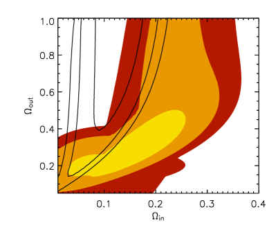
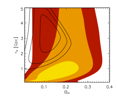
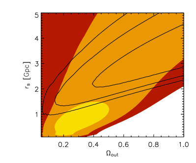
Figure 2: The best fit on-center LTB models. The upper left panel shows $\Omega_{\rm M}(r)$ and $H_{0}(r)$ as a function of the radial coordinate. The other panels show the 68.3, 95 and 99 % confidence contours (for two parameters) for the model parameters $\Omega_{\rm in}$, $\Omega_{\rm out}$ and $r_{\rm s}$. The contours are given in colour for the SDSS-II data set and with solid black lines for the Constitution set.

The best fit LTB model to the SDSS-II data set for an on-center observer has the best fit parameters $\Omega_{\rm in}=0.16$, $\Omega_{\rm out}=0.29$ and $r_{\rm s}=0.7$ Gpc (corresponding to $z\approx 0.16$) with $\chi^{2}=229.3$. In comparison, the best fit flat $\Lambda$CDM model has $\chi^{2}=231.3$. For the Constitution set the best fit LTB model has $\Omega_{\rm in}=0.13$, $\Omega_{\rm out}=1$ and $r_{\rm s}=3.5$ Gpc (corresponding to $z\approx 1.02$) with $\chi^{2}=461.0$. Here the flat $\Lambda$CDM model gives $\chi^{2}=465.5$. Figure 2 shows the results for the two data sets. The top left panel shows the functions $\Omega_{\rm M}(r)$ and $H_{0}(r)$ and illustrates well the big difference between the best fit models. Whereas the SDSS-II data are best fit with a moderately large void with a small change in the matter density, the Constitution set prefers an asymptotically flat model with a very large void. The other panels show the 68.3, 95 and 99 % two parameter confidence contours (corresponding to $\Delta\chi^{2}=[2.30,5.99,9.21]$) for the model parameters, with the SDSS-II contours presented in colour and the Constitution contours overplotted with solid lines. There is a clear tension between the data sets, with no overlap of the 68.3 % contours. This difference in results is partly a consequence of the different redshift distributions, but also an effect of the light-curve fitter used. If we impose the prior of asymptotic flatness, $\Omega_{\rm out}=1$, the SDSS-II fit becomes notably worse, with $\chi^{2}=234.6$. The local matter density changes to $\Omega_{\rm in}=0.23$ and the scale radius is pushed up to a whopping $r_{\rm s}=4.8$ Gpc. For the Constitution set this prior does not make a difference, since an asymptotically flat model is already preferred by the fit.

The best fits to the data sets are also illustrated in the Hubble diagrams in Figure 3. For comparison, we have included the best fit flat $\Lambda$CDM models, and for the SDSS-II case we have also plotted the best fit asymptotically flat LTB model. It is quite striking how the data differ between the panels. The difference in the best fit parameter values for the data sets can be appreciated fairly intuitively from this figure. For the SDSS-II data set (left panel), the new SNe Ia at intermediate redshifts trace out a bump centered around $z\sim 0.25$, which largely dictates the size of the void. A smaller void would place the bump at too low redshift, while a larger void would move the bump to higher redshift and make it less pronounced. At higher redshifts, i.e., in the regime where $\Omega_{\rm M}(r)$ is essentially constant, the curve follows close to a straight line. The low value of $\Omega_{\rm out}=0.29$, ensures that it doesn’t fall off too fast and misses the high-$z$ data bins. The Constitution set (right panel), on the other hand, contains few SNe Ia at intermediate redshifts, but instead features twice as many SNe Ia as the SDSS-II between $z=0.4$ and $z=0.9$. These give a very broad bump centered around $z\sim 0.6$ in the Hubble diagram. The data is best fit with a very large void together with a high value for $\Omega_{\rm out}$. A smaller void would place the bump at lower redshift, while a decrease in the asymptotic matter density would flatten out the curve.

Figure 3: Hubble diagrams for the best fit on-center models (solid). Distance modulus differences in magnitudes are shown with respect to an empty universe. The data have been binned for visualization purposes using $n\Delta z=5$, where $n$ is the number of SNe Ia in the bin and $\Delta z$ the redshift range. The data points are located at the mean value of the redshifts and the weighted mean of the distance moduli. The redshift error bars show the standard deviation of the redshifts in the bin, while the distance modulus error bars give the error of the weighted mean of the distance moduli within the bin. The best fit flat $\Lambda$CDM models (dashed) are included for comparison. For the SDSS-II case, we also show the best fit asymptotically flat ($\Omega_{\rm out}=1$) LTB model (dot-dashed).

We also mention that we have investigated the Gaussian LTB model previously for the case of an on-center observer and ranked it against the most commonly considered dark energy models [33]. We used the SDSS-II data set but also included constraints from the cosmic microwave background and the baryon acoustic oscillations in the analysis. While the LTB model could provide a fit that was comparable to those of the dark energy models, it was not preferred from a model selection point of view since extra parameters are required.

5 Solving the geodesic equation for off-center observers

We now wish to calculate the luminosity distance to a SN Ia as seen by an observer located off-center in the void. We define the origin of the coordinate system to be at the void center and choose the $z$-axis in the direction of the off-center observer. The coordinates of any space-time point in this frame are the time coordinate $t$, the radial coordinate $r$, the polar angle $\theta$ and the azimuthal angle $\phi$. This means that the spatial coordinates of the observer in this frame are $r=r_{\rm obs}$, $\theta=0$ and a degenerate $\phi$. Infalling photons hit the observer at time $t_{0}$, polar angle $\gamma$ and azimuthal angle $\xi$. We need to trace these photons back along their trajectories to the source. The redshift of the SN Ia refers to what the off-center observer measures, such that $z(r_{\rm obs})=0$.

The system of differential equations that we need to solve in order to obtain the coordinates of the SN Ia as a function of redshift is derived in A,

$$\frac{dt}{dz}=-\frac{(1+z)}{q}\ ,$$ (12)

$$\frac{dr}{dz}=\frac{p}{q}\ ,$$ (13)

$$\frac{d\theta}{dz}=\frac{J}{qA^{2}}\ ,$$ (14)

$$\frac{dp}{dz}=\frac{1}{q}\Bigg{[}\frac{(1-k)}{A^{\prime}}\frac{J^{2}}{A^{3}}+\frac{2\dot{A}^{\prime}}{A^{\prime}}p(1+z)-\Bigg{(}\frac{A^{\prime\prime}}{A^{\prime}}+\frac{k^{\prime}}{2-2k}\Bigg{)}p^{2}\Bigg{]}\ ,$$ (15)

under the constraint

$$q=\Bigg{[}\frac{A^{\prime}\dot{A}^{\prime}}{1-k}p^{2}+\frac{\dot{A}J^{2}}{A^{3}}\Bigg{]}\ ,$$ (16)

where $p\equiv dr/d\lambda$, with $\lambda$ being an affine parameter along the geodesic. The constant angular momentum $J$ can be calculated as [22]

$$J=A(r_{0},t_{0})\sin\gamma\ .$$ (17)

The initial conditions used for the off-center observer are

$$t_{0}=t_{\rm BB}$$ (18)

$$r_{0}=r_{\rm obs}$$ (19)

$$\theta_{0}=0$$ (20)

$$p_{0}=\frac{\sqrt{1-k(r_{0})}}{A^{\prime}(r_{0},t_{0})}\cos\gamma\ .$$ (21)

The SN Ia positions in the sky are in the equatorial coordinate system given by the right ascension $\alpha$ and declination $\delta$. We need to relate these angles to the coordinate system of the void. The polar angle $\gamma$ seen by the off-center observer can be obtained as

$$\cos\gamma=-\sin\beta\sin(90^{\circ}-\delta)\cos(\alpha+\sigma)+\cos\beta\cos(90^{\circ}-\delta)\ ,$$ (22)

where $\beta$ is the inclination angle between the $z$-axis and the celestial equator’s normal and $\sigma$ is the angle between the $x$-axis and the vernal equinox point. The orientation angles $\beta$ and $\sigma$ determine the position of the void center and are free parameters in the fit. With these definitions, the void center is located at $\alpha_{\rm c}=360^{\circ}-\sigma$ and $\delta_{\rm c}=90^{\circ}-\beta$ in the equatorial coordinate system. In moving the observer away from the void center, we have thus introduced three new free parameters in the fit; the radial displacement $r_{\rm obs}$ and the orientation angles $\beta$ and $\sigma$.

Finally, the expression for calculating the angular diameter distance is modified for the case of an off-center observer to [23],

$$d_{\rm A}^{4}=\frac{A^{4}\sin^{2}\theta}{\sin^{2}\gamma}\Bigg{[}\frac{A^{\prime 2}}{A^{2}(1-k)}\Bigg{(}\frac{\partial r}{\partial\gamma}\Bigg{)}^{2}+\Bigg{(}\frac{\partial\theta}{\partial\gamma}\Bigg{)}^{2}\Bigg{]}\ ,$$ (23)

where the partial derivatives are obtained numerically in the solution of the geodesic equations.

6 Constraining the observer position with SNe Ia

Off-center observers will see an anisotropic relation between the luminosity distance and the redshift for the SNe Ia. This means that a standard candle with the same redshift but in different directions in the sky will have different observed magnitudes. The isotropy of the data can be used to establish constraints on the observer position inside the void. In this section, we will investigate how far from the center the observer can be located.

6.1 Maximum anisotropy

Figure 4: Magnitude dipole induced by moving the observer away from the void center in the best fit on-center models. The curves show the difference in magnitude for two SNe Ia with the same redshift but in opposite directions in the sky. Left panel: A void with scale radius $r_{\rm s}=0.7$ Gpc ($z\approx 0.18$), preferred by the SDSS-II data set. Right panel: A void with scale radius $r_{\rm s}=3.5$ Gpc ($z\approx 1.02$), preferred by the Constitution data set.

To get a sense for how big the effect of being situated off-center has on the SN Ia observations, we can calculate the maximum anisotropy in the form of the magnitude dipole. We take two SNe Ia with the same redshift but in opposite directions in the sky, aligned with the off-center observer through the void center. Figure 4 shows the magnitude dipole, i.e., the difference in magnitude between the two SNe Ia for three different redshifts as a function of the radial displacement of the observer. We have used the best fit on-center models for the SDSS-II (left panel), where $r_{\rm s}=0.7$ Gpc ($z\approx 0.16$), and the Constitution data set (right panel), where $r_{\rm s}=3.5$ Gpc ($z\approx 1.02$).

The behaviour of the curves is easily understood. For on-center observers, the universe is isotropic and the magnitude dipole vanishes. For observers located very far from the center, the magnitude dipole becomes less significant. The curves reach a maximum at some displacement, depending on the redshift. Figure 4 demonstrates that SNe Ia at different redshifts have different constraining power when determining the observer position. For the smaller void preferred by the SDSS-II data, the largest anisotropies are obtained for SNe Ia at $z=0.1$. The difference in brightness can be larger than 0.1 magnitudes if the observer is located a few hundred Mpc from the center. SNe Ia at larger redshifts are less affected by the off-center position. SNe Ia at low to intermediate redshifts will provide the strongest constraints on the observer position in this case. In the much larger void obtained for the Constitution set, SNe Ia at $z=0.4$ display the largest anisotropy. An observer located about 1-2 Gpc from the center would see a magnitude dipole of around 0.3 magnitudes for these SNe Ia. For this void, the strongest constraints on the observer position come from SNe Ia at intermediate to high redshift. These conclusions also hold for the SDSS-II fit when we impose a prior of asymptotic flatness on the model.

6.2 Results

Figure 5: The changes in the $\chi^{2}$ values relative to the on-center value as a function of the observer position. The stars show the angle-optimized values when the void model is kept fixed to the best fit on-center parameter values. The diamonds show the void model-optimized values when the angles are kept fixed to the angle-optimized values. The scale radius of the void is $r_{\rm s}=0.7$ Gpc for the SDSS-II set (left panel) and $r_{\rm s}=3.5$ Gpc for the Constitution set (right panel).

We displace the observer from the center and make new fits to the data sets. Figure 5 shows the changes in the $\chi^{2}$ values compared to the on-center value, as a function of the observer position. In the first case (denoted as fixed model) we take the best fit on-center model and displace the observer in different directions, i.e., we scan the parameters $r_{\rm obs}$, $\beta$ and $\sigma$ for a fixed void model. The stars show the lowest $\chi^{2}$ value obtained for each value of $r_{\rm obs}$. Note that the scale radius of the void is very different for the two data sets, with $r_{\rm s}=0.7$ Gpc for the SDSS-II set and $r_{\rm s}=3.5$ Gpc for the Constitution set. For the SDSS-II (left panel) we find that the fit improves over the on-center case out to about $r_{\rm obs}=250$ Mpc, which corresponds to 36 % of the scale radius. The best fit has $\Delta\chi^{2}=-0.5$ for $r_{\rm obs}=100$ Mpc and the void center at $(\alpha_{\rm c},\delta_{\rm c})=(200^{\circ},-50^{\circ})$ in equatorial coordinates or $(l_{\rm c},b_{\rm c})=(308^{\circ},13^{\circ})$ in galactic coordinates. For the Constitution set (right panel) we find that the fit improves over the on-center case out to about $r_{\rm obs}=320$ Mpc, which corresponds to 9 % of the scale radius. The best fit has $\Delta\chi^{2}=-1.6$ for $r_{\rm obs}=160$ Mpc and the void center at $(\alpha_{\rm c},\delta_{\rm c})=(350^{\circ},-50^{\circ})$ in equatorial coordinates or $(l_{\rm c},b_{\rm c})=(334^{\circ},-61^{\circ})$ in galactic coordinates.

As presented in section 4, the best fit to the SDSS-II data for an on-center observer in an asymptotically flat model is a huge void with $r_{\rm s}=4.8$ Gpc that has $\Delta\chi^{2}=5.3$ compared to the non-flat model. If we displace the observer in such a model, the best fit instead has $\Delta\chi^{2}=0.3$ for $r_{\rm obs}=600$ Mpc (13 % of the scale radius). A model with an off-center observer in an asymptotically flat void can thus provide a fit that is comparable to that of an on-center observer in a non-flat void. Note, however, that this requires three additional parameters.

In the second case (denoted as fixed position) we use the orientation angles that gave the lowest $\chi^{2}$ values in the previous case and instead optimize the void model, i.e., we scan the parameters $\Omega_{\rm in}$, $\Omega_{\rm out}$ and $r_{\rm s}$ for a fixed position. Using this approach it is possible to improve the fits further. For the SDSS-II (left panel of Figure 5), the fit is improved all the way out to $r_{\rm obs}\sim 550$ Mpc. As the observer is displaced further and further from the center, the best fit parameters change to lower values for $\Omega_{\rm in}$ and $\Omega_{\rm out}$, and larger values for $r_{\rm s}$. For the Constitution set (right panel) the fit is improved out to $r_{\rm obs}\sim 400$ Mpc. The changes in $\Omega_{\rm in}$ and $r_{\rm s}$ are only small and the model remains asymptotically flat.

We would like to point out that we have not performed a full high-resolution parameter scan over all six parameters simultaneously, so we expect that it is possible to find (slighty) lower $\chi^{2}$ values than what we have presented here and we refrain from giving precise quantitative limits on how far we can be from the center at a certain level of confidence. Regardless, our results show that SN Ia data allow for off-center observers and that the fit in fact can be improved for such a scenario. For the Constitution set the observer can be displaced $\sim$15 % of the scale radius from the center and still yield an acceptable fit to the data. For the SDSS-II set a tolerable fit can be obtained for observers displaced all the way out to around the scale radius. However, given that three additional parameters for the observer position have been introduced, without providing a substantial improvement of the fit, we cannot claim that the off-center model is preferred from a model selection point of view.

7 Constraining the observer position with SNe Ia and the CMB dipole

Being situated away from the center of the void induces anisotropies in the CMB temperature [22]. So far we have disregarded this effect in the analysis and focused purely on the SN Ia data. In this section we will continue to investigate the constraints on the observer position coming from the SNe Ia observations while simultaneously accommodate the CMB dipole anisotropy measurement. This can be achieved by introducing a peculiar velocity of the observer directed to counterbalance the dipole induced by the off-center position. Here we will impose that the void model is asymptotically flat, $\Omega_{\rm out}=1$, in order to be consistent with constraints on the spatial curvature derived from measurements of the CMB.

7.1 CMB dipole and peculiar velocity

The COBE satellite measured the average CMB temperature across the sky to be $T_{0}=2.725$ K and the amplitude of the temperature fluctuations to $\Delta T=3.353$ mK [34]. The main contribution to the CMB temperature anisotropies comes from the dipole, which is in the direction $(l,b)=(264.26^{\circ},48.22^{\circ})$ in galactic coordinates or $(\alpha,\delta)=(168.05^{\circ},-7.06^{\circ})$ in equatorial coordinates. In a homogeneous universe, the CMB dipole is attributed to a velocity, $v_{\rm d}$, of the observer relative to the comoving coordinates,

$$\frac{v_{\rm d}}{c}=\frac{\Delta T}{T_{0}}\ .$$ (24)

The COBE measurements imply that $v_{\rm d}=369$ km s^-1 (corresponding to the net velocity of the Sun relative to the CMB). The measured redshifts of the SNe Ia have been corrected for this velocity in the data sets, so that they are given in a frame at rest with respect to the CMB.

In the LTB scenario, the inhomogeneous expansion can be interpreted to cause a velocity, $v_{\rm h}$, of the off-center observer relative to the void center [22],

$$\frac{v_{\rm h}}{c}=\frac{H_{0,\rm in}-H_{0,\rm out}}{c}r_{\rm obs}\ .$$ (25)

In this picture, it is thus the observer’s position in an inhomogeneous universe, and not primarily a coordinate velocity, that induces the measured CMB dipole. The CMB photons arriving from the far side of the void will travel longer through a region with larger expansion rate and will thus be redshifted. This means that the CMB temperature measured in the direction of the void center will be lower compared to that measured in the opposite direction. The void center is then located at $(\alpha_{\rm c},\delta_{\rm c})=(348.05^{\circ},7.06^{\circ})$ and the orientation angles are $\beta=82.94^{\circ}$ and $\sigma=11.95^{\circ}$.

It is possible to introduce a peculiar velocity, $v_{\rm p}$, of the observer, directed towards the void center, as a counterbalance in order to allow for larger off-center displacements without violating the CMB dipole measurement. The requirement is thus that it is the net effect of the off-center position and the peculiar velocity that gives rise to the observed dipole,

$$\vec{v}_{\rm h}+\vec{v}_{\rm p}=\vec{v}_{\rm d}\ .$$ (26)

The introduction of a peculiar velocity, directed along the z-axis, will also affect the SN Ia measurements. For a given SN Ia, the measured redshift $z$ and luminosity distance $d_{\rm L}$ have to be translated into their cosmological counterparts $\bar{z}$ and $\bar{d_{\rm L}}$ according to [35]

$$1+z=(1-v_{\rm p}\cos\gamma)(1+\bar{z})\ ,$$ (27)

$$d_{\rm L}=\bar{d_{\rm L}}(\bar{z})(1+v_{\rm p}\cos\gamma)(1-v_{\rm p}\cos\gamma)^{2}\ .$$ (28)

We have neglected the peculiar velocities of the SNe Ia. In the fitting procedure we must thus take the measured redshift and obtain the cosmological redshift using equation (27), calculate the corresponding cosmological luminosity distance, and finally translate this value according to equation (28) in order to compare to the measured luminosity distance.

7.2 Results

Figure 6: The changes in the $\chi^{2}$ values for the fit to the SNe Ia as a function of the observer’s position. The stars show the values when the static observer is displaced in the direction of the CMB dipole in the best fit on-center LTB model. The diamonds show the values when the observer also has a peculiar velocity directed to accommodate the observed CMB dipole. The arrows indicate the direction of motion, either away from the void center or towards it. The vertical dotted line shows the position where the peculiar velocity is zero. The scale radius of the void is $r_{\rm s}=5.0$ Gpc for the SDSS-II set (left panel) and $r_{\rm s}=3.7$ Gpc for the Constitution set (right panel).

We make new model fits for the case of a static on-center observer in an asymptotically flat void, using the measured redshifts instead of the redshifts corrected to the CMB frame provided in the data set. The best fit to the SDSS-II set has $\chi^{2}=231.5$ and the best fit parameters are $\Omega_{\rm in}=0.22$ and $r_{\rm s}=5.0$ Gpc. For the Constitution set, the best fit has $\chi^{2}=471.5$, with $\Omega_{\rm in}=0.13$ and $r_{\rm s}=3.7$ Gpc.

Using these best fit on-center models, Figure 6 shows how the $\chi^{2}$ values change compared to the on-center value as the observer is displaced from the center in the direction of the CMB dipole. In the first case (denoted as static) the observer has no peculiar velocity and the CMB dipole requirement is disregarded. These points only serve as a comparison in the plot. In the second case (denoted as moving) the observer has a peculiar velocity that perfectly balances the off-center position so that the dipole requirement of equation (26) is fulfilled at all values of $r_{\rm obs}$. The arrows indicate the direction of the velocity, either away from the void center or towards it. The vertical dotted line marks the position where the peculiar velocity is zero. Figure 6 demonstrates the power of combining the SNe Ia data with the CMB dipole requirement when constraining the observer position. While the induced CMB dipole can always be balanced with an appropriately directed peculiar velocity, this motion will simultaneously affect the quality of the fit to the SNe Ia. For the SDSS-II set (left panel) the peculiar velocity is zero at $r_{\rm obs}=28.7$ Mpc. Introducing a peculiar velocity leads to a deterioration of the fit compared to the static case. The best fit is obtained for $r_{\rm obs}=25$ Mpc, which corresponds to 0.5 % of the scale radius. The observer thus has a small peculiar velocity directed away from the void center for this fit. While smaller displacements can give comparable fits, the $\chi^{2}$ value quickly increases as the observer is displaced further from the center. For the Constitution set (right panel) the peculiar velocity is zero at $r_{\rm obs}=23$ Mpc. The peculiar velocity leads to an improvement of the fit for smaller displacements compared to the static case. The best fit is obtained for $r_{\rm obs}=6$ Mpc, which is only 0.2 % of the scale radius. The observer has a sizeable peculiar velocity directed away from the void center for this fit. The $\chi^{2}$ value increases quickly as the observer is displaced further from the center.

We conclude that in order to obtain a good fit to the SN Ia data and simultaneously accommodate the CMB dipole requirement, the observer must be located within $\sim$1 % of the scale radius.

8 Conclusions

We have considered off-center observers in a large, spherically symmetric local void described by the LTB metric and investigated the constraints on the observer position placed by SNe Ia. The analysis was performed using two supernova data sets, the first-year SDSS-II data set and the Constitution data set, which differ in the redshift distribution and the number of SNe Ia, as well as the light-curve fitter used in order to obtain the peak magnitudes. Models with an on-center observer were able to provide good fits which had slightly lower $\chi^{2}$ values than those obtained for the flat $\Lambda$CDM model, but the best fit voids look very different for the two data sets. Whereas the SDSS-II data prefer a moderately large void and a low value of the asymptotic matter density, the Constitution set is best fit with an asymptotically flat model with a very large void. By displacing the observer from the center we found that the data indeed allow for off-center observers. For the SDSS-II set the fit was improved out to 36 % of the scale radius and for the Constitution set out to 9 %, the stronger constraint placed by the Constitution set as expected from the larger number of SNe Ia and the more isotropic sky distribution. However, for both data sets the improvement of the fit was only marginal. Using SN Ia data alone, we conclude that the observer can be displaced at least 15 % of the void scale radius from the center and still give an acceptable fit to the data. These conclusions are in good agreement with those reached in Alnes & Amarzguioui [23]. We have also performed the analysis using a different parameterisation of the density profile [15] with very similar results.

In the final part of the analysis we also took into consideration that the off-center position induces anisotropies in the CMB temperature. While the requirement that the induced CMB dipole must be consistent with the measured value can always be accommodated by introducing a balancing peculiar velocity of the observer, such a motion simultaneously affects the SN Ia observations. Using this combination of the CMB dipole measurement and the SNe Ia data, we were able to determine very strict constraints on how far from the center the observer can be located. The best fits were obtained for an observer located at 0.5 % of the scale radius for the SDSS-II data set and 0.2 % of the scale radius for the Constitution data set. In order to still get a good fit to the SN Ia data, the observer must be within about 1 % of the scale radius.

Our more general conclusion is that within the void model, observers have to live very close to the center in order for the model to accomodate the data. Besides requiring an uncomfortable amount of fine-tuning, such a scenario also constitutes a severe challenge to the Copernican principle that we should not occupy a special place in the universe.

In the future, we expect new and better data from many independent cosmological probes to put the LTB models to even greater challenges, including new model constraints from large SN Ia data sets with extensive sky coverage also at higher redshifts. LTB models may ultimately prove to not be viable cosmological models, but they can at least serve as a specific set of toy models to gauge the influence of large-scale matter inhomogeneities on the light propagation. Such effects are indubitably present as systematic errors in the observations and it is important to be able to quantify their significance in order to further advance precision cosmology.

Appendix A The geodesic equations

The photon paths are governed by the geodesic equation. Alnes & Amarzguioui [22] derived the differential equations for the time coordinate $t$, radial coordinate $r$ and polar angle $\theta$ in the LTB space-time,

$$\frac{d^{2}t}{d\lambda^{2}}+\frac{A^{\prime}\dot{A}^{\prime}}{1-k}\Bigg{(}\frac{dr}{d\lambda}\Bigg{)}^{2}+A\dot{A}\Bigg{(}\frac{d\theta}{d\lambda}\Bigg{)}^{2}=0\ ,$$ (29)

$$\frac{d^{2}r}{d\lambda^{2}}+\Bigg{(}\frac{A^{\prime\prime}}{A^{\prime}}+\frac{k^{\prime}}{2-2k}\Bigg{)}\Bigg{(}\frac{dr}{d\lambda}\Bigg{)}^{2}+\frac{2\dot{A}^{\prime}}{A^{\prime}}\frac{dr}{d\lambda}\frac{dt}{d\lambda}-\frac{A(1-k)}{A^{\prime}}\Bigg{(}\frac{d\theta}{d\lambda}\Bigg{)}^{2}=0\ ,$$ (30)

$$\frac{d}{d\lambda}\Bigg{(}A^{2}\frac{d\theta}{d\lambda}\Bigg{)}\equiv\frac{d}{d\lambda}J=0\ ,$$ (31)

where the paths are parameterized by the affine parameter $\lambda$ and equation (31) has been written as conservation of angular momentum $J$. Note that due to axial symmetry, the photon paths are independent of the azimuth angle $\phi$. Furthermore, the equation for the redshift $z$ reads as

$$\frac{dz}{d\lambda}=-(1+z)\frac{d\lambda}{dt}\Bigg{[}\frac{A^{\prime}\dot{A}^{\prime}}{1-k}\Bigg{(}\frac{dr}{d\lambda}\Bigg{)}^{2}+A\dot{A}\Bigg{(}\frac{d\theta}{d\lambda}\Bigg{)}^{2}\Bigg{]}\ .$$ (32)

By introducing $u\equiv dt/d\lambda$ and $p\equiv dr/d\lambda$, we can bring equations (29) and (30) down to first order, and the set of differential equations can then be written as

$$\frac{du}{d\lambda}=-\Bigg{[}\frac{A^{\prime}\dot{A}^{\prime}}{1-k}p^{2}+A\dot{A}\Bigg{(}\frac{J}{A^{2}}\Bigg{)}^{2}\Bigg{]}\ ,$$ (33)

$$\frac{dp}{d\lambda}=\frac{A(1-k)}{A^{\prime}}\Bigg{(}\frac{J}{A^{2}}\Bigg{)}^{2}-\frac{2\dot{A}^{\prime}}{A^{\prime}}pu-\Bigg{(}\frac{A^{\prime\prime}}{A^{\prime}}+\frac{k^{\prime}}{2-2k}\Bigg{)}p^{2}\ ,$$ (34)

$$\frac{d\theta}{d\lambda}=\frac{J}{A^{2}}\ ,$$ (35)

$$\frac{dz}{d\lambda}=-(1+z)\frac{1}{u}\Bigg{[}\frac{A^{\prime}\dot{A}^{\prime}}{1-k}p^{2}+A\dot{A}\Bigg{(}\frac{J}{A^{2}}\Bigg{)}^{2}\Bigg{]}\ .$$ (36)

Combining Eqs. (33) and (36) yields

$$u=u_{0}(1+z)\ ,$$ (37)

where we can choose $u_{0}=u(\lambda=0)=-1$.

We want to solve for the coordinates as a function of redshift, and this can be achieved since

$$\frac{d}{d\lambda}=\frac{dz}{d\lambda}\frac{d}{dz}\equiv q\frac{d}{dz}\ .$$ (38)

We can now write down the system of differential equations that we need to solve to obtain $t(z)$, $r(z)$, $\theta(z)$ and $p(z)$,

$$\frac{dt}{dz}=\frac{u_{0}(1+z)}{q}\ ,$$ (39)

$$\frac{dr}{dz}=\frac{p}{q}\ ,$$ (40)

$$\frac{d\theta}{dz}=\frac{J}{qA^{2}}\ ,$$ (41)

$$\frac{dp}{dz}=\frac{1}{q}\Bigg{[}\frac{(1-k)}{A^{\prime}}\frac{J^{2}}{A^{3}}-\frac{2\dot{A}^{\prime}}{A^{\prime}}pu_{0}(1+z)-\Bigg{(}\frac{A^{\prime\prime}}{A^{\prime}}+\frac{k^{\prime}}{2-2k}\Bigg{)}p^{2}\Bigg{]}\ ,$$ (42)

under the constraint

$$q\equiv\frac{dz}{d\lambda}=-\frac{1}{u_{0}}\Bigg{[}\frac{A^{\prime}\dot{A}^{\prime}}{1-k}p^{2}+\frac{\dot{A}J^{2}}{A^{3}}\Bigg{]}\ .$$ (43)

References

References

- [1] SUPERNOVA SEARCH TEAM collaboration, Riess A G et al, Observational Evidence from Supernovae for an Accelerating Universe and a Cosmological Constant, Astron. J. 116 (1998) 1009
- [2] SUPERNOVA COSMOLOGY PROJECT collaboration, Perlmutter S et al, Measurements of Omega and Lambda from 42 High-Redshift Supernovae, Astrophys. J. 517 (1999) 565
- [3] WMAP collaboration, Komatsu E et al, Five-Year Wilkinson Microwave Anisotropy Probe Observations: Cosmological Interpretation, Astrophys. J. Suppl. 180 (2009) 330
- [4] SDSS collaboration, Eisenstein D et al, Detection of the Baryon Acoustic Peak in the Large-Scale Correlation Function of SDSS Luminous Red Galaxies, Astrophys. J. 633 (2005) 560
- [5] Percival W et al, Measuring the Baryon Acoustic Oscillation scale using the Sloan Digital Sky Survey and 2dF Galaxy Redshift Survey, Mon. Not. Roy. Astron. Soc. 381 (2007) 1053
- [6] Célérier M-N, The Accelerated Expansion of the Universe Challenged by an Effect of the Inhomogeneities. A Review, [astro-ph/0702416]
- [7] Lemaître G, L’Univers en expansion, Annales Soc. Sci. Brux. 53 (1933) 51
- [8] Lemaître G, The Expanding Universe, Gen. Rel. Grav. 29 (1997) 641
- [9] Tolman R C, Effect of Inhomogeneity on Cosmological Models, Proc. Nat. Acad. Sci. 20 (1934) 169
- [10] Bondi H, Spherically symmetrical models in general relativity, Mon. Not. Roy. Astron. Soc. 107 (1947) 410
- [11] Hunt P and Sarkar S, Constraints on large-scale inhomogeneities from WMAP5 and SDSS: confrontation with recent observations, Mon. Not. Roy. Astron. Soc. 401 (2010) 547
- [12] Enqvist K and Mattsson T, The effect of inhomogeneous expansion on the supernova observations, JCAP 02 (2007) 019
- [13] Clifton T, Ferreira P G and Land K, Living in a Void: Testing the Copernican Principle with Distant Supernovae, Phys. Rev. Lett. 101 (2008) 131302
- [14] Alnes H, Amarzguioui M and Grøn Ø, Inhomogeneous alternative to dark energy?, Phys. Rev. D 73 (2006) 083519
- [15] Garcia-Bellido J and Haugbølle T, Confronting Lemaitre Tolman Bondi models with observational cosmology, JCAP 04 (2008) 003
- [16] Bolejko K and Wyithe J S B, Testing the copernican principle via cosmological observations, JCAP 02 (2009) 020
- [17] Garcia-Bellido J and Haugbølle T, The radial BAO scale and Cosmic Shear, a new observable for Inhomogeneous Cosmologies, JCAP 09 (2009) 028
- [18] Zibin J P, Moss A and Scott D, Can We Avoid Dark Energy?, Phys. Rev. Lett. 101 (2008) 251303
- [19] February S et al, Rendering Dark Energy Void, arXiv:0909.1479 [astro-ph]
- [20] Caldwell R R and Stebbins A, A Test of the Copernican Principle, Phys. Rev. Lett. 100 (2008) 191302
- [21] Garcia-Bellido J and Haugbølle T, Looking the void in the eyes - the kinematic Sunyaev Zeldovich effect in Lemaître Tolman Bondi models, JCAP 09 (2008) 016
- [22] Alnes H and Amarzguioui M, CMB anisotropies seen by an off-center observer in a spherically symmetric inhomogeneous universe, Phys. Rev. D 74 (2006) 103520
- [23] Alnes H and Amarzguioui M, Supernova Hubble diagram for off-center observers in a spherically symmetric inhomogeneous universe, Phys. Rev. D 75 (2007) 023506
- [24] Quercellini C, Quartin M and Amendola L, Possibility of Detecting Anisotropic Expansion of the Universe by Very Accurate Astrometry Measurements, Phys. Rev. Lett. 102 (2009) 151302
- [25] Kessler R et al, First-year Sloan Digital Sky Survey-II (SDSS-II) Supernova Results: Hubble Diagram and Cosmological Parameters, Astrophys. J. Suppl. 185 (2009) 32
- [26] Jha S, Riess A G and Kirshner R P, Improved Distances to Type Ia Supernovae with Multicolor Light-Curve Shapes: MLCS2k2, Astrophys. J. 659 (2007) 122
- [27] ESSENCE collaboration, Wood-Vasey W M et al, Observational Constraints on the Nature of Dark Energy: First Cosmological Results from the ESSENCE Supernova Survey, Astrophys. J. 666 (2007) 694
- [28] The SNLS collaboration, Astier P et al, The Supernova Legacy Survey: measurement of , and w from the first year data set, Astron. Astrophys. 447 (2006) 31
- [29] Riess A G et al, New Hubble Space Telescope Discoveries of Type Ia Supernovae at z 1: Narrowing Constraints on the Early Behavior of Dark Energy, Astrophys. J. 659 (2007) 98
- [30] Hicken M et al, Improved Dark Energy Constraints from 100 New CfA Supernova Type Ia Light Curves, Astrophys. J. 700 (2009) 1097
- [31] SUPERNOVA COSMOLOGY PROJECT collaboration, Kowalski M et al, Improved Cosmological Constraints from New, Old, and Combined Supernova Data Sets, Astrophys. J. 686 (2008) 749
- [32] Hicken M et al, CfA3: 185 Type Ia Supernova Light Curves from the CfA, Astrophys. J. 700 (2009) 331
- [33] Sollerman J et al, First-Year Sloan Digital Sky Survey-II (SDSS-II) Supernova Results: Constraints on Nonstandard Cosmological Models, Astrophys. J. 703 (2009) 1374
- [34] Bennett C L et al, Four-Year COBE DMR Cosmic Microwave Background Observations: Maps and Basic Results, Astrophys. J. 464 (1996) L1
- [35] Haugbølle T et al, The Velocity Field of the Local Universe from Measurements of Type Ia Supernovae, Astrophys. J. 661 (2007) 650