Anderson localization transition and eigenfunction multifractality in ensemble of ultrametric random matrices.

Abstract

We demonstrate that by considering disordered single-particle Hamiltonians (or their random matrix versions) on ultrametric spaces one can generate an interesting class of models exhibiting Anderson metal-insulator transition. We use the weak disorder virial expansion to determine the critical value of the parameters and to calculate the values of the multifractal exponents for inverse participation ratios. Direct numerical simulations agree favourably with the analytical predictions.

A metric space is called ultrametric, if a distance function $d(x,y)$ satisfies the strong triangle inequality $d(x,y)\leq\max\{d(x,z),d(z,y)\}$ for any three points $x$, $y$ and $z$, so that all triangles are either isosceles or equilateral. The notion of ultrametricity appears naturally in $p$-adic analysis [1] which plays important role in various branches of mathematics and string theory. Ultrametric spaces have found many useful applications in physics and beyond [2], most notably in the theory of spin glasses [3] where they describe the hierarchical organization of free energy landscapes. Random matrices whose structure reflects some specific aspects of ultrametricity were under active study recently due to their relevance to description of relaxation properties in complex landscapes typical for heteropolymers and related systems [4].

The aim of the present work is to demonstrate that by considering disordered single-particle Hamiltonians (or their random matrix versions) on ultrametric spaces one can generate an interesting class of models exhibiting Anderson metal-insulator transition. The latter is one of the central phenomena in the theory of disordered quantum systems and describes an abrupt change in the nature of eigenstates from extended to spatially localized. Exactly at the transition point eigenstates are very inhomogeneous and strongly fluctuating and can be characterized by non-trivial multifractal dimensions. Despite a great progress in understanding of the Anderson transition achieved in the last decades [5] based mainly on the mapping to the nonlinear $\sigma-$model [6, 7], there are still relatively few models of disordered Hamiltonians exhibiting the localisation transition and affordable for direct analytical studies. Among those deserving special mentioning are the models on the infinite tree-like graph (Bethe lattice) [7, 8] and the ensemble of power-law banded random matrices introduced in [9] and further investigated in [10] which became rather popular in recent years. The problem of rigorous mathematical analysis of the Anderson transition is yet outstanding, see e.g. [11].

The idea that models of statistical mechanics on hierarchical spaces with effectively ultrametric structure can be efficiently studied analytically due to their high symmetry goes back to Dyson[12] and proved to be rather useful in shedding light on renormalisation group methods and developing rigorous mathematical proofs in general theory of phase transitions [13]. Recently there was a systematic attempt to put disordered models of spin-glass type on such lattices [14]. We hope that the models proposed in the present paper will provide a useful framework for further insights into the nature of the Anderson localisation transition, and perhaps could yield to a rigorous mathematical analysis.

Let us start by introducing a random matrix ensemble of Hermitian matrices with ultrametric structure whose eigenvectors exhibit the Anderson transition when changing some control parameter. The idea behind such an approach is that ensembles of that sort can be not only efficiently studied numerically, but should be also amenable to a variety of existing analytical techniques like, for example, mapping to a kind of nonlinear $\sigma-$model on ultrametric space, which could keep promise for an exact solution (see a short discussion in the end of the paper). Leaving the investigation of these issues to a future research, in this paper we are to exploit some recent analytical insights provided by works on almost-diagonal random matrices [15, 16].

The ultrametric structure for a particular representative $H$ of the suggested ensemble of random matrices is encoded in the choice of variances for the Gaussian-distributed entries. Namely, all $2^{K}\times 2^{K}$ entries $H_{ij}$ of the matrix $H$ are taken as independent complex Gaussian random variables (up to the obvious Hermiticity constraint $H_{ij}^{\ast}=H_{ji}$) with the zero mean value. All diagonal elements of $H$ are real and have the same variance: $\left\langle H_{ii}^{2}\right\rangle=W^{2},\,\forall i$. The variances of the off-diagonal elements have a block structure typical for ”hierarchic” lattices (Fig. 1a), with blocks of the sizes $1,2,2^{2},\ldots,2^{K-1}$. Inside each block of the size $2^{l}$ the variances $\left\langle H_{ij}^{\ast}H_{ij}\right\rangle$ are constant and chosen to be $J^{2}/p^{2l}$, controlled by two real parameters $J$ and $p$. Such a random matrix describes random hopping between boundary nodes of a tree of $K$ generations with given coordination number which we choose for simplicity to be equal to two (Fig. 1b) . The underlying tree serves the purpose of defining the ultrametric distance $d(i,j)$ between any pair of boundary nodes. It is defined as the number of edges in the shortest path connecting nodes $i$ and $j$. As easy to check the corresponding distance is ultrametric. The formula for the variances can be then expressed naturally in terms of $d(i,j)$ as $\left\langle H_{ij}^{\ast}H_{ij}\right\rangle=J^{2}/p^{d(i,j)-2}$.

(a) (b)

Figure 1: (a) Schematic structure of variances of entries of an ultrametric random matrix. (b) Hopping between nodes of the ultrametric lattice.

The ultrametric random matrix model introduced above exhibits the Anderson transition by changing parameter $p$. Namely, in the thermodynamic limit $K\to\infty$ the eigenvectors of $H$ are extended for $p<2$, localized for $p>2$ and critical (multifractal) at $p=2$ . We expect this scenario to hold for any ratio $J/W$, implying in particular that at $p=2$ changing $J/W$ should allow to pass from strongly to weakly multifractal eigenstates. Assuming that $J/W\ll 1$, the fractal dimensions $d_{q}$ of the eigenvectors (defined below in Eqs.(Anderson localization transition and eigenfunction multifractality in ensemble of ultrametric random matrices.-3)) in the critical regime can be calculated explicitly and are given by:

$$d_{q}=\frac{J}{W}\frac{\sqrt{\pi}}{\sqrt{2}\ln 2}\frac{\Gamma(q-1/2)}{\Gamma(q)},\quad q>\frac{1}{2},$$ (1)

where $\Gamma(q)$ is the Euler Gamma-function.

We define the moments of the eigenvector components $I_{q}$ (also known as inverse participation ratios, IPR’s) in the standard way:

$$I_{q}(E) = \frac{1}{N}\sum_{n=1}^{N}P_{q}(E,n)$$

$$P_{q}(E,n) = \frac{1}{\rho(E)}\sum_{k=1}^{N}|\Psi_{k}(n)|^{2q}\delta(E-E_{k}),$$ (2)

where the normalized eigenvectors $\Psi_{k}$ with $N\equiv 2^{K}$ components $\Psi_{k}(n),\,n=1,2,\ldots,N$ correspond to the eigenvalues $E_{k}$ and $\rho(E)$ stands for the mean density of states at the energy $E$ (which will be fixed to zero for simplicity). At criticality the ensemble-averaged moments of the eigenvectors scale anomalously with the system size $N$, defining a set of fractal dimensions $d_{q}$:

$$\left\langle I_{q}\right\rangle\propto N^{-d_{q}(q-1)}.$$ (3)

In order to calculate the moments of the eigenvectors under the condition $J/W\ll 1$ we use the method of the virial expansion developed in [16, 17]. The methods allows us to construct a well-controlled perturbation expansion of the moments of the eigenvectors using the small parameter $J/W$. The first term of the expansion is generated by the diagonal part of a matrix $H$. All corresponding eigenvectors have only one non-zero component, which is equal to one due to the normalization condition. As a result all moments of the eigenvectors are equal to one in this approximation: $\left\langle I_{q}^{(0)}\right\rangle=1$. The corrections to this result originating from the off-diagonal matrix elements of $H$ can be represented as certain integrals over commuting and anti-commuting variables. That integrals can be either calculated explicitly [16, 17] or alternatively they can be interpreted as the moments of the eigenvectors of certain submatrices of a matrix $H$. To be specific, the lowest order in $J/W$ correction $I_{q}^{(1)}$ is generated by the following $2\times 2$ sub-matrices of $H$:

$$H(n,m) = \left(\begin{array}[]{cc}H_{nn}&H_{nm}\\ H_{nm}^{\ast}&H_{mm}\end{array}\right),n,m=1,\dots,N,\quad n\neq m$$ (6)

Denoting by $P_{q}(n,m)$ the moments of the first component of the corresponding eigenvectors we are able to represent $\left\langle I_{q}^{(1)}\right\rangle$ as follows:

$$\left\langle I_{q}^{(1)}\right\rangle=\frac{1}{N}\sum_{n\neq m}^{N}(\left\langle P_{q}(n,m)\right\rangle-1)$$ (7)

The subtraction of unity is required in order to get rid of the contribution already taken into account at the previous step. The above approximation implies that the pair-wise ”interaction” of the levels of the unperturbed system is taken into account at this stage. Essentially the same idea was underlying the real-space renormalization approach developed for critical systems with a long-range interaction and the power-law random banded matrix model [18, 10].

Below we calculate the averaged value of $I_{q}^{(1)}$ using an explicit expression for the eigenvectors components. To this end let us introduce the following notation $E_{1}\equiv H_{nn}$, $E_{2}\equiv H_{mm}$, $h\equiv H_{nm}$ and $P_{q}\equiv P_{q}(n,m)$. The eigenvalues $\lambda_{1}$, $\lambda_{2}$ of the matrix $H(n,m)$ are equal to

$$\lambda_{1,2}=\frac{1}{2}(E_{1}+E_{2}\pm\sqrt{(E_{1}-E_{2})^{2}+4|h|^{2}}).$$ (8)

The absolute values of the components $\psi_{1,2}$ of the corresponding normalised eigenvectors are given by $|\psi_{1,2}|=\frac{|h|}{\sqrt{|h|^{2}+(\lambda-E_{1,2})^{2}}}$. Averaging the moments of $|\psi_{1}|$ first over $E_{1}$ and $E_{2}$ we obtain the following expression for $\left\langle P_{q}\right\rangle_{E}$:

$$\left\langle P_{q}\right\rangle_{E}=\int\int_{-\infty}^{\infty}\frac{dE_{1}dE_{2}}{2\pi\rho W^{2}}\sum_{i=1}^{2}\frac{e^{-\frac{E_{1}^{2}+E_{2}^{2}}{2W^{2}}}|h|^{2q}\delta(\lambda_{i})}{(|h|^{2}+(\lambda_{i}-E_{1})^{2})^{q}},$$ (9)

where $\rho$ is the density of states at $E=0$. The latter can be easily calculated in the diagonal approximation giving the result $\rho=1/\sqrt{2\pi}W$. The corrections generated by off-diagonal elements of $H$ is of the order of $(J/W)^{2}$ [15] and hence can be neglected. Eq.(8) shows that $\lambda_{1}=0$ if $E_{1}E_{2}=|h|^{2}$ and $E_{1}+E_{2}\leq 0$, while $\lambda_{2}=0$ if $E_{1}E_{2}=|h|^{2}$ and $E_{1}+E_{2}\geq 0$. Therefore we should consider separately two domains of integration $E_{1}+E_{2}\leq 0$ and $E_{1}+E_{2}\geq 0$. In each domain only one of the $\delta$-functions in Eq.(9) survives. After a simple change of variables we are able to integrate over $E_{1}$ in Eq.(9):

$$\left\langle P_{q}\right\rangle_{E} = \int_{-\infty}^{\infty}\frac{dE_{2}}{\sqrt{2\pi}W}e^{-\frac{|h|^{4}+E_{2}^{4}}{2W^{2}E_{2}^{2}}}\left(\frac{E_{2}^{2}}{E_{2}^{2}+|h|^{2}}\right)^{q-1}=$$ (10)

$$= \int_{-\infty}^{\infty}\frac{dx\>|h|}{\sqrt{2\pi}W}e^{-\frac{|h|^{2}}{2W^{2}}\left(\frac{1}{x^{2}}+x^{2}\right)}\left(\frac{x^{2}}{x^{2}+1}\right)^{q-1},$$

where the new variable of integration $x=|h|E_{2}$ is introduced. Now we are ready to perform averaging over the complex variable $h$. Since the expression above depends only on $|h|$ the integration over the argument $h$ is trivial and just leads to appearance of the factor $2\pi$ while integration over $|h|$ can be done explicitly:

$$\left\langle P_{q}\right\rangle_{E,h}=\frac{\alpha}{2}\int_{-\infty}^{\infty}dx\frac{\left(x^{-2}+1\right)^{1-q}}{\left(1+\alpha\left(x^{-2}+x^{2}\right)\right)^{3/2}},$$ (11)

where $\alpha\equiv\sqrt{\left\langle|h|^{2}\right\rangle}/\sqrt{2}W$. The asymptotic behaviour of this expression in the limit $\alpha\to 0$ has the following form:

$$\left\langle P_{q}\right\rangle_{E,h}=1-\sqrt{\pi}\frac{\Gamma(q-1/2)}{\Gamma(q-1)}\alpha+O(\alpha^{2}).$$ (12)

The first term in the expansion corresponds to the diagonal approximation and is cancelled by $-1$ in Eq.(7), while the second one gives a non-trivial contribution. Collecting the results of Eqs.(Anderson localization transition and eigenfunction multifractality in ensemble of ultrametric random matrices.,7,12) we find $\left\langle I_{q}\right\rangle$ up to the first order in $J/W$:

$$\left\langle I_{q}\right\rangle = 1-\sqrt{\frac{\pi}{2}}\frac{\Gamma(q-1/2)}{\Gamma(q-1)}\frac{1}{N}\sum_{n\neq m}^{N}\frac{\sqrt{\left\langle|H_{nm}|^{2}\right\rangle}}{W}$$ (13)

$$= 1-\frac{J}{W}\sqrt{\frac{\pi}{2}}\frac{\Gamma(q-1/2)}{\Gamma(q-1)}\sum_{m=2}^{N}\frac{1}{p^{d(1,m)/2-1}}.$$ (14)

According to the definition of the ultrametric distance $d(n,m)$ the sum in Eq.(14) is given by the geometric series:

$$S\equiv\sum_{m=2}^{N}\frac{1}{p^{d(1,m)/2-1}}=\sum_{i=0}^{K-1}\left(\frac{2}{p}\right)^{i}=\frac{\left(\frac{2}{p}\right)^{K}-1}{\frac{2}{p}-1}.$$ (15)

As $K\to\infty$ the asymptotic behaviour of the above sum crucially depends on the value of the parameter $p$: for $p>2$ the sum tends to the finite value $S\to p/(p-2)<\infty$ independent of $N$ implying that eigenvectors are localized, whereas in opposite situation $p<2$ we see that $S$ diverges as $S\approx(p/(2-p))N^{1-\log_{2}{p}}$, signalling of a breakdown of the perturbation theory for arbitrarily weak off-diagonal coupling. It is natural to interpret such breakdown as the signal of eigenvector delocalization. Finally, at the critical point $p=2$ we have $S=K=\log_{2}N$ leading to

$$\left\langle I_{q}\right\rangle=1-\frac{J}{W}\sqrt{\frac{\pi}{2}}\frac{\Gamma(q-1/2)}{\Gamma(q-1)}\log_{2}N.$$ (16)

Comparing this result with the definition of $d_{q}$ given by Eq.(3), and expecting $d_{q}\ll 1$ for $J/W\ll 1$ we interpret this marginal behaviour in terms of the anomalous scaling of the moments of the eigenvectors, and the expression for the fractal dimensions (1) immediately follows. The condition $q>1/2$ is necessary to guarantee the convergence of the derivative with respect to $\alpha$ of the integral in (11) at $\alpha=0$. One expects that the region $q<1/2$ can be covered by employing the powerful symmetry relation discovered in [19] , see below.

One can notice that the $q$-dependence of the above expression is exactly the same as the one found for the ensemble of the power-law random banded matrices [10]. The matrix elements of that ensemble are independently distributed Gaussian variables with zero mean and with variance decaying in a power-law fashion as a function of the distance to the main diagonal. Such a coincidence can be easily explained by Eq.(13). Indeed, we can see that $q$-dependence enters only in the pre-factor and thus is always the same for any Gaussian ensemble with independent entries. However we would like to stress that this ”superuniversal” behaviour should be expected only in the regime $J/W\ll 1$.

The results of numerical simulations confirming our predictions are presented in Fig. 2. The moments of the eigenvectors, whose eigenvalues are close to $E=0$, were calculated for various system sizes ranging from $N=2^{8}$ to $N=2^{14}$. To obtain their averaged values reliably a large number of random matrices were generated, so that the number of eigenvectors contributing to the computed averaged values were ranged from $10^{3}$ for $N=2^{14}$ up to $10^{5}$ for $N=2^{8}$. The extracted values of the fractal dimensions $d_{q}$ for $J=1$, $W=10$ and $W=1/3$ are represented in Fig. 2 by circles and triangles respectively. For $q<0$ the eigenstates intensities were first coarse-grained over boxes containing $8$ sites. The values of $d_{q}$ for $W=10$ are in perfect agreement with our analytical prediction (solid line in Fig. 2). The latter was calculated directly from Eq.(1) for $q>1/2$. To make the prediction for $q<1/2$ we used the remarkable symmetry relation discovered in [19] and intimately related to profound fluctuation relations in the field of non-equilibrium dynamics [20]. According to it the anomalous multifractal exponent defined as $\Delta_{q}\equiv(d_{q}-d)(q-1)$, where $d$ is the dimensionality of the space, is symmetric with respect to line $q=1/2$, i.e. $\Delta_{q}=\Delta_{1-q}$. In our model $d=1$, as according to Eq.(3) the fractal dimensions are defined by the scaling of the moments of the eigenvectors with respect to the total number of sites $N$ (“volume” of the system). We checked the validity of the relation for our model (inset of Fig. 2) and employed it to calculate $d_{q}$ for $q<1/2$ analytically using Eq.(1). The fact that the expression (1) diverges at $q=1/2$ indicates that our perturbative approach breaks down at some values $q_{\ast}$ close to $q=1/2$, at which Eq.(1) becomes of the order of one. However we would like to mention that the values $q_{\ast}$ can be made arbitrary close to $1/2$ by taking $J/W$ sufficiently small.

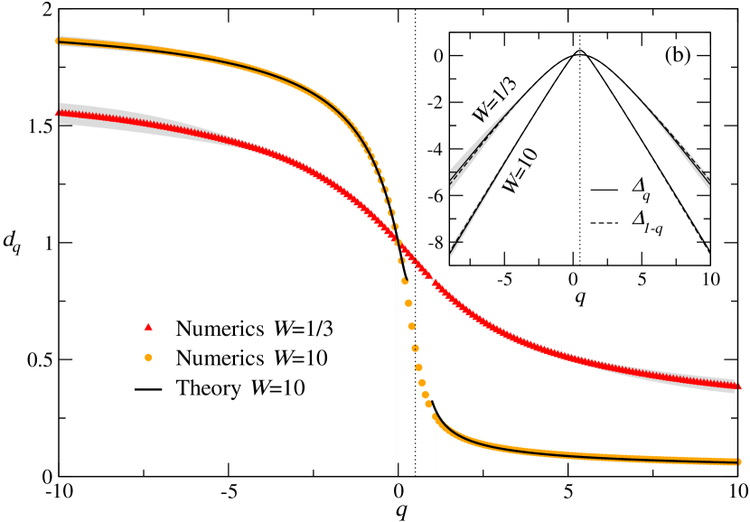
Figure 2: Fractal dimensions $d_{q}$ for $J=1$, $W=10$ (circles) and $W=1/3$ (triangles). The solid line is the analytical prediction based on Eq.(1). Inset: numerically calculated exponents $\Delta_{q}$ (solid) and $\Delta_{1-q}$ (dashed). The gray shaded background marks the 95% confident interval of the numerical results.

Another possible realization of the ultrametricity in the framework of disordered systems is the ultrametric Anderson model, which is a version of the Anderson model defined on the lattice of $N=2^{K}$ sites supplied with the ultrametric distance $d(i,j)$ described above. The diagonal matrix elements of the Hamiltonian are assumed to be random and characterized by the variance $W$. The off-diagonal matrix elements $H_{ij}$ of the Anderson model are however non-random. Their values $H_{ij}=J/p^{d(i,j)/2-1}$ depend on two parameters $J$ and $p$ and the distance $d(i,j)$ similar to corresponding variances of an ultrametric random matrix.

Although one can not apply directly our results to the Anderson model, one can use the argument due to Levitov [18] to establish the existence of the Anderson transition for this model. According to that argument, two sites $i$ and $j$ will be mixed by the off-diagonal entries of ${\cal H}$ only when they are ”in resonance”: $|H_{ii}-H_{jj}|<H_{ij}$. It is easy to estimate the probability that two sites are in resonance:

$$P_{ij}=\int\int\frac{dH_{ii}dH_{jj}}{2\pi W^{2}}e^{-H^{2}_{ii}/2W^{2}-H^{2}_{jj}/2W^{2}}\theta\left(H_{ij}-|H_{ii}-H_{jj}|\right)$$ (17)

where $\theta(x)$ is the step-function. Calculating the integral yields $P_{ij}=\sqrt{\frac{2}{\pi}}\int_{0}^{H_{ij}/\sqrt{2}W}e^{-x^{2}/2}\,dx\approx\sqrt{\frac{2}{\pi}}\frac{H_{ij}}{W}$ in our approximation. Then the mean total number of sites $\left\langle\#\right\rangle_{i}$ which are in resonance with a given site $i$ is given by:

$$\left\langle\#\right\rangle_{i}=\sum_{j\neq i}P_{ij}=\sqrt{\frac{2}{\pi}}\frac{1}{W}\sum_{j\neq i}\,H_{ij}$$ (18)

When the number $\left\langle\#\right\rangle_{i}$ is divergent in the limit $N\to\infty$ as a power of $N$ the couplings, whatever weak, produce delocalization of eigenvectors in the site basis. On the other hand that number tending to a finite limit indicates localization of the corresponding eigenvectors in the weak coupling limit (which of course does not preclude possibility of delocalization at some critical coupling). Finally, the transition between the two regimes happens precisely when $\left\langle\#\right\rangle_{i}\sim\ln{N}$. For the ultrametric Anderson model $\sum_{j\neq i}H_{ij}/W=(J/W)S$, where $S$ is defined by Eq.(15). Thus we conclude that depending on $p$ the nature of the eigenvectors of the Anderson model is the same as for its random matrix analogue: localized for $p>2$, extended for $p<2$ and critical at $p=2$, although we expect the dependence of anomalous dimensions $d_{q}$ on the parameter $J/W$ to be different in the two models. The statistics of energy level spacings is expected to be Poisson for $p>2$ and Wigner-Dyson for $p<2$. For earlier studies of spectral properties of the random Schroedinger-like operators with hierarchical structure see [21, 22].

Finally, let us say a few words about possibilities to understand the opposite limit of strong off-diagonal coupling $J\gg W$. In the original formulation of the model neglecting diagonal entries does not seem to lead to any essential simplification, and we are unfortunately unable to provide any insights to the problem. However, one can think of introducing an ”n-orbital” variant of our model in the spirit of [6]. In this way one should replace each entry $H_{ij}$ of the hierarchical random matrix Hamiltonian with $n\times n$ block of independent, identically distributed zero mean Gaussian elements with the variances $J^{2}/p^{2l}$ inherited from the original $n=1$ model. Letting $n\to\infty$ and simultaneously rescaling the parameters $J$ and $W$ in such a way that $J^{2}/W^{2}=t/n$ with some $t=O(1)$ ensures a non-trivial limit of the theory equivalent to a lattice version of the standard nonlinear $\sigma-$model, with couplings depending on the ultrametric distance between the lattice sites. In such approach the strong coupling limit $t\gg 1$ will be amenable to the standard perturbative expansion in diffusion-like modes like in [9], with the diffusion propagator replaced by its analogue on the hierarchical lattice (note that as the model lacks the translation invariance the standard Fourier modes expansion is ineffective and should be replaced by a certain ultrametric analogue). We leave analysis of this and related questions to subsequent publications.

AO acknowledges support from the EPSRC [EP/G055769/1]. YF is grateful to S. Nechaev for triggering his interest in hierarchical models. AR gratefully acknowledge funding from EPSRC (EP/C007042/1).

References

References

- [1] Brekke L and Freund P 1993 Phys. Rep. 233 1
- [2] Rammal R, Toulouse G and Virasoro M A, 1986 Rev. Mod. Phys. 58 765
- [3] Mezard M, Parisi G and Virasoro M A 1987 Spin Glass Theory and Beyond (Singapore: World Scientific)
- [4] Avetisov V A, Bikulov A Kh and Nechaev S K, 2009 J. Phys. A 42 075001; Avetisov V A, Chertovich A V, Nechaev S K and Vasilyev O A 2009 J. Stat. Mech. P07008; Avetisov V A, Bikulov A Kh, Vasilyev O A, Nechaev S K and Chertovich A V 2009 Zh. Eksp. Teor. Fiz. 1̱36 566
- [5] Evers F and Mirlin A D 2008 Rev. Mod. Phys. 80 1355
- [6] Wegner F 1979 Zeitsch. Physik 36 207; Schäfer L and Wegner F 1980 Zeitsch. Phys. B 38 113
- [7] Efetov K B 1997 Supersymmetry in Disorder and Chaos (Cambridge: Cambridge University Press).
- [8] Abou-Chacra R, Anderson P W, Thouless D J 1973 J. Phys. C 6 1734; Zirnbauer M R 1986 Phys. Rev. B 34 6394; Mirlin A D and Fyodorov Y V 1991 Nucl. Phys. B 366 507; Klein A 1998 Adv. in Math. 133 163
- [9] Mirlin A D, Fyodorov Y V, Dittes F M, Quezada J and Seligman T H 1996 Phys. Rev.E 54 3221
- [10] Mirlin A D and Evers F 2000 Phys. Rev.B 62 7920
- [11] Disertori M, Spencer T and Zirnbauer M 2009 Preprint arXiv:0901.1652
- [12] F.J. Dyson, Comm. Math. Phys. 12 91 (1969), and ibid 212 ;
- [13] Collet P and Eckman J-P 1978 A Renormalization group analysis of the hierarchical model in statistical mechanics Lecture Notes in Physics 74 (Springer-Verlag, 1978, 199pp) and references therein; Bleher P M and Major P 1987 The Annals of Probability 15 431.
- [14] Franz S, Jörg T and Parisi G 2009 J. Stat. Mech. P02002
- [15] Yevtushenko O and Kravtsov V E 2003 J. Phys. A 36 8265
- [16] Yevtushenko O and Ossipov A 2007 J. Phys. A 40 4691
- [17] Ossipov A, Yevtushenko O and Kravtsov V E, in preparation.
- [18] Levitov L S 1990 Phys. Rev. Lett.64 547
- [19] Mirlin A D, Fyodorov Y V, Mildenberger A and Evers F 2006 Phys. Rev. Lett. 97 046803
- [20] Monthus C, Berche B, and Chatelain C 2009 Preprint arXiv:0909.0584
- [21] Molchanov S 1996 Proc. of the 6th Lukacs Simposium (ed. A.K. Gupta and V.A. Girko, VSP, 1996) pp. 179-192
- [22] Kritchevski E 2007 Proc. Amer. Math. Soc. 135 1431; Kritchevski E 2007 Probability and Mathematical Physics 42 309