D-brane Inspired Fermion Mass Textures

In this paper, the issues of the quark mass hierarchies and the Cabbibo Kobayashi Maskawa mixing are analyzed in a class of intersecting D-brane configurations with Standard Model gauge symmetry. The relevant mass matrices are constructed taking into account the constraints imposed by extra abelian symmetries and anomaly cancelation conditions. Possible mass generating mechanisms including perturbative as well as non-perturbative effects are discussed and specific patterns of mass textures are found characterized by the hierarchies of the scales where the various sources contribute. It is argued that the Cholesky decomposition of the mass matrices is the most appropriate way to determine the properties of these fermion mass patterns, while the associated triangular mass matrix form provides a unified description of all phenomenologically equivalent symmetric and non-symmetric mass matrices. An elegant analytic formula is derived for the Cholesky triangular form of the mass matrices where the entries are given as simple functions of the mass eigenstates and the diagonalizing transformation entries. Finally, motivated by the possibility of vanishing zero Yukawa mass entries in several D-brane and F-theory constructions due to the geometry of the internal space, we analyse in detail all possible texture-zeroes mass matrices within the proposed new context. These new texture-zeroes are compared to those existing in the literature while D-brane inspired cases are worked out in detail.

1 On the fermion mass problem

One of the most fascinating challenges in gauge theories of fundamental interactions today, is the implementation of a natural mechanism providing a satisfactory explanation of the observed hierarchical fermion mass spectrum and quark mixing. Concentrating on the hadronic sector in particular, we know today experimentally with remarkable accuracy the quark masses and the Cabbibo Kobayashi Maskawa (CKM) mixing which arises because the Yukawa matrices are not diagonal in flavor space. This mixing determines the strengths of the transitions between the various quark flavors explaining the observations related to the CP-violation in the neutral Kaon system and other interesting processes involving quark flavor physics .

Since the birth of modern gauge theories and the establishment of the Standard Model, the problem of mass hierarchy and flavor mixing have been tackled in many ways. Among the various attempts, abelian and several discrete symmetries [2] were often ‘mobilized’ to discriminate fermion families, supplying thus the theory with more or less realistic textures which reproduce the observed fermion mass spectrum.

It was subsequently shown that such $U(1)$ family symmetries arise naturally in the context of string models . As a result, a generic characteristic of these constructions is that at the tree-level superpotential only one fermion generation (usually the third) of Yukawa couplings is allowed. The remaining two fermion families obtain their masses from higher order non-renormalizable (NR) terms when the various singlet or any other Higgs fields appearing in the string spectrum obtain vacuum expectation values (vevs), breaking thus the surplus $U(1)$ symmetries and filling in the tree-level zeroes of the mass matrices with subleading mass terms. As the latter are mainly correlated to the lighter generations a consistent quark mass hierarchy arises in a natural way.

Searching for simplicity and maximal predictability on the fermion mass problem, a purely phenomenological approach restricted to symmetric matrices only, revealed that admissible fermion mass textures can be classified to five texture-zero mass matrices which contain all relevant information and reproduce the low energy measurements [8]. All these textures exhibit a hierarchical structure in the sense that the magnitudes of the non-zero entries coupled to heavier generations are bigger than those coupled to the lighter ones.

D-brane models however have paved the way for new interesting possibilities. Recently, a closer look at the phenomenological properties of the predicted superpotential terms has revealed that completely novel structures of non-symmetric mass matrices may appear [9],[10],[11],[12],[13],[14],[15].

In a wide class of these constructions this mainly happens because of constraints originating not only from $U(1)$ symmetries, but also from restrictions imposed by tadpole and other anomaly cancelation conditions. For example, in D-brane models built in the context of the Standard Model symmetry, quark and lepton fields should be distributed between equal numbers of $N$ and $\bar{N}$ representations. If we confine ourselves to cases of D-brane configurations with the minimal SM spectrum, we find that the consrtaints are automatically satisfied for the $SU(3)$ color group, however, the implementation for the case of the $SU(2)$ doublets imposes additional restrictions on the Yukawa sector. These restrictions lead to rather peculiar mass matrix structures where the magnitudes of the non-zero entries do not follow a hierarchical pattern in the sense that was described above.

Some of these models may prove to be ephemeral, but, they undoubtedly indicate that there are lots of surprises on the way, thus a detailed analysis towards a complete classification of mass matrix textures consistent with the fermion masses and mixing is needed.

In the present paper, motivated by recent activity on D-brane phenomenological explorations related to the origin of fermion masses and their hierarchies, we elaborate on the issue of fermion mass spectrum in SM D-brane variants and develop a method to construct new viable mass textures, concentrating mainly on the quark sector. Our results, are more general and can be applied to the charged lepton and the neutrino sector as well. We treat symmetric and non-symmetric mass matrices on an equal footing, by working out the triangular (Cholesky) form of the admissible mass matrices which encodes all the physical properties in a unique way. It is shown that all matrix elements can be analytically expressed in terms of simple unique functions of the quark masses and the corresponding elements of diagonalizing matrix. This latter (Cholesky) form of the $3\times 3$ fermion mass textures can be considered to act as a progenitor of equivalent classes of admissible symmetric and non-symmetric matrices connected by orthogonal matrices acting on it.

We further pursue our approach by using the Cayley-Hamilton theorem to develop a new more compact formalism for the orthogonal transformations that facilitates the analysis of the diagonalizing matrices and reveals the geometrical nature of the multiplication properties on computations regarding the Cabbibo-Kobayashi-Maskawa mixing and the quark mass spectrum. Thus geometrical treatment provides also the tools to investigate cases where up and down quark matrices are misaligned and considerable adjustments are necessary to obtain the CKM mixing. This happens for example in F-theory constructions [16],[17], when matter curves for up and down quarks intersect at different points [18]-[20].

In the present analysis we will not deal with corrections attributed to renormalization group evolution. Thus, for demonstration purposes, experimentally measured quantities (like masses and mixing) at the electroweak scale will be used as if the mass matrices were obtained at low energy scales. This is very reasonable for D-brane models with low unification scale, however, more precise quantitative estimates for high unification scale scenarios can be easily obtained by taking into account the radiative corrections which can be easily parametrized in terms of one parameter only [8].

The present paper is organized as follows: In section 2 we derive the Yukawa superpotential in the context of a Standard Model variant emerging from a simple D-brane configuration and construct the quark mass matrices with the aforementioned characteristics. A short exploration of the magnitude of the Yukawa terms with respect to their particular origin is carried out and a new vector-like parametrization of the matrices is proposed which facilitates the subsequent analysis. A characteristic case of the derived quark mass textures is worked out is detail and the compatibility of the findings with the low experimental energy data are discussed. In section 3 we introduce the Cholesky form of the mass matrices and explore the mathematical properties which will enable us to classify the admissible quark mass textures. We show how the triangular (Cholesky) form of a mass matric acts as a ‘progenitor’ of an equivalent class of symmetric and non-symmetric mass matrices with the same ‘physical’ properties, i.e., the same eigenmasses and mixing. Then, in section 4 we introduce a new parametrization of the orthogonal transformations and use the analysis of the previous section to express analytically the entries of the triangular matrix as functions of the mass eigenstates and the diagonalizing matrix elements. An investigation on simplified phenomenologically viable texture-zero forms of the triangular matrix is made in section 5. A separate discussion is also devoted on comparison issues of the present approach and the symmetric texture-zeroes in the existing literature. The conditions on the parameter space in a class of texture-zeroes matrices to obtain consistency of the D-brane inspired matrices and examples are worked out in detail in section 6. In section 7 we present our conclusions while in section 8 we include further details of our calculations.

2 Quark mass textures in a class of intersecting D-brane models

In order to demonstrate the existence of the novel class of mass matrices in this section we proceed with the analysis of the Yukawa sector of one particular example based on the simplest and most economical D-brane configuration which can incorporate the Standard Model (SM) gauge symmetry. We should point out however, that the peculiar textures derived here are by no means a narrow characteristic of this chosen model. Delving into the variety of the D-brane SM constructions, one can find that this specific mass pattern appears in a wide class of intersecting D-brane SM models [9],[10], in Gepner constructions [11],[14] as well as in certain GUTs [13].

In all those D-brane analogues of the old successful gauge models, additional restrictions are imposed on the matter representations due to the tadpole and anomaly cancelation conditions. More precisely, for any $U(N_{j})$ factor of the gauge symmetry $G_{S}=\prod_{j}U(N_{j})$, implied by a D-brane configuration, tadpole cancelation conditions demand equal number of $N_{j}$ and $\bar{N}_{j}$ representations.

In the case of D-brane successors of the Standard Model gauge symmetry  with minimal quark and charged lepton sector, as far as the $U(3)$ representations are concerned, this requirement is automatically satisfied. Furthermore, in order to implement this condition for the $U(2)$ gauge factor, one has to discriminate between $SU(2)$ doublet and anti-doublet fields and ensure that equal numbers are predicted for both in the massless spectrum. As a consequence, at least in the simplest and more appealing cases with the minimal spectrum, not all quark doublet fields arise from the same intersection, and therefore matter fields belonging to different generations definitely carry unrelated $U(1)$ quantum numbers.

In this context, simple hierarchical symmetric textures which were usually discussed in the literature are far from being realistic and one has to confront the mass texture problem in a more general context. In this section we demonstrate this fact by giving one such simple example implying representative quark mass textures of these constructions.

We assume a D-brane configuration [10] with three stacks (call them $a,b,c$) which generatethe $U(3),U(2),U(1)$, gauge symmetries respectively (the relevant D-brane configuration is depicted in figure 1).

Figure 1: A depiction of the $U(3)\times U(2)\times U(1)$ D-brane configuration with strings representing the SM states. For the sake of simplicity, $a,b,c$ denote $U(3),U(2)$ and $U(1)$ branes respectively. In this figure D-branes are not distinguished from their corresponding mirrors. Thus, the blue string representing the quark doublet $Q^{\prime}$ is stretched between the $D6_{a}$ and the mirror $D6_{b^{*}}$. Similarly, one endpoint of the “$d^{c}$-string” is attached on the mirror $D6_{c^{*}}$.

These are sufficient to incorporate the Standard Model gauge symmetry together with its minimal fermion and Higgs spectrum which is shown in Table 1. This consists of the three SM fermion generations, enlarged by the corresponding right handed neutrinos and one pair of Higgs doublets. It can be checked that anomaly cancelation conditions are also satisfied.

Inters.	$SU(3)\times SU(2)$	${\cal Q}_{a}$	${\cal Q}_{b}$	${\cal Q}_{c}$	$Y$
$ab$	$1\times Q\,(3,\bar{2})$	$1$	$-1$	$0$	$\frac{1}{6}$
$ab^{*}$	$2\times Q^{\prime}\,(3,2)$	$1$	$1$	$0$	$\frac{1}{6}$
$ac$	$3\times u^{c}\,(\bar{3},1)$	$-1$	$0$	$1$	$-\frac{2}{3}$
$ac^{*}$	$3\times d^{c}\,(\bar{3},1)$	$-1$	$0$	$-1$	$\frac{1}{3}$
$bc$	$3\times L\,(1,\bar{2})$	$0$	$-1$	$1$	$-\frac{1}{2}$
$cc^{*}$	$3\times e^{c}\,(1,1)$	$0$	$0$	$-2$	$1$
$bb^{*}$	$3\times\nu^{c}\,(1,1)$	$0$	$-2$	$0$	$0$
$bc^{*}$	$\left.\begin{array}[]{r}1\times H_{d}(1,2)\\ 1\times{H}_{u}(1,\bar{2})\end{array}\right.$	$\left.\begin{array}[]{r}0\\ 0\end{array}\right.$	$\left.\begin{array}[]{r}1\\ -1\end{array}\right.$	$\left.\begin{array}[]{r}1\\ -1\end{array}\right.$	$\left.\begin{array}[]{r}-\frac{1}{2}\\ \frac{1}{2}\end{array}\right.$

Table 1: The quantum numbers of the SM fermions in the $U(3)\times U(2)\times U(1)$ brane configuration. The last column is the Hypercharge $Y=\frac{1}{6}{\cal Q}_{a}-\frac{1}{2}{\cal Q}_{c}$ while three previous ones refer to the $U(1)$ charges with respect to the $a,b,c$ brane-stacks.

Let $Q_{p}^{\prime}=(3,2),\;p=1,2$ and $Q=(3,\bar{2})$ the three quark doublets and $u_{j}^{c},d_{j}^{c},j=1,2,3$ the right-handed partners. The tree-level quark and lepton Yukawa couplings of this construction are

$${\cal W}\supset\lambda^{u}_{pj}\,Q_{p}^{\prime}\,u^{c}_{j}\,H_{u}+(\lambda^{d}_{j}\,Q\,d^{c}_{j}+\lambda^{l}_{ij}\,L_{i}\,e^{c}_{j})H_{d}$$ (1)

In the first term, the indices $i,j$ run over all three fermion generations, while $p$ takes only two values, not yet assigned to particular fermion generations. Thus, only two quark-doublet flavors contribute through tree-level perturbative Yukawa couplings to the up-quark mass matrix. The reason is that the additional $U(1)_{a}$ charges carried by the various representations do not allow for a coupling involving the representation $Q(3,\bar{2})$. For the same reason tree-level mass terms for the two quark doublets do not appear in the down quark mass matrix, since the down right-handed quarks couple only to the remaining quark doublet. As can be inferred, there is a complementary texture zero structure of the up and down quark mass matrices at the perturbative level, in the sense that the zero entries of the first are non-zero in the second and vice versa. Of course this structure could not be acceptable since it would definitely lead to a zero mass for one up and two down quarks, thus additional contributions should be expected from other sources like those discussed above. Thus, the zero entries are expected to be filled in by elements generated by some other mechanism. The main sources are 1) an additional Higgs doublet pair, 2) NR-terms obtained when singlet Higgs fields are introduced in the spectrum or 3) when stringy instanton effects are taken into account.

If any of the above mechanisms is implemented, the following Yukawa terms could be included to the superpotential

$${\cal W}^{\prime} = {\lambda^{\prime}}_{j}^{u}\,Q\,u_{j}^{c}\,H_{u}^{\prime}+{\lambda^{\prime}}_{pj}^{d}\,Q^{\prime}_{p}\,d^{c}_{j}\,H_{d}^{\prime}+\cdots$$ (2)

where the $j$ and $p$ indices in (2) span the flavor numbers exactly as in (1). These new terms are sufficient to provide the missing entries in the quark mass matrices while dots refer to other possible generated terms (i.e. Dirac-type neutrino masses etc) which do not concern us here. The crucial observation however, is that the order of magnitude of these new terms (2) is expected to differ from those of (1), since their origin is different.

Taking into account the tree-level perturbative and the additional terms (2), the up and down quark mass textures are classified into three distinct classes depending on the particular family assignment. Hence, the first class arises assuming that $Q^{\prime}(3,2)$ accommodates the lightest generation so we have

$$\frac{m_{Q}}{\langle H_{u}\rangle}=\left(\begin{array}[]{lll}\kappa_{u}\eta_{11}^{u}&\kappa_{u}\eta_{12}^{u}&\kappa_{u}\eta_{13}^{u}\\ \lambda_{21}^{u}&\lambda_{22}^{u}&\lambda_{23}^{u}\\ \lambda_{31}^{u}&\lambda_{32}^{u}&\lambda_{33}^{u}\end{array}\right),\;\frac{m_{D}}{\langle H_{d}\rangle}=\left(\begin{array}[]{lll}\lambda_{11}^{d}&\lambda_{12}^{d}&\lambda_{13}^{d}\\ \kappa_{d}\eta_{21}^{d}&\kappa_{d}\eta_{22}^{d}&\kappa_{d}\eta_{23}^{d}\\ \kappa_{d}\eta_{31}^{d}&\kappa_{d}\eta_{32}^{d}&\kappa_{d}\eta_{33}^{d}\end{array}\right)$$ (9)

where, for later convenience, we have written ${\lambda_{j}^{\prime}}^{u}=\kappa^{u}\eta^{u}_{1j}$ and ${\lambda^{\prime}}_{pj}^{d}=\kappa^{d}\eta_{pj}^{d}$ with $p=2,3$ and $j=1,2,3$. The remaining two possibilities are

$$\frac{m_{Q}}{\langle H_{u}\rangle}=\left(\begin{array}[]{lll}\lambda_{11}^{u}&\lambda_{12}^{u}&\lambda_{13}^{u}\\ \kappa_{u}\eta_{21}^{u}&\kappa_{u}\eta_{22}^{u}&\kappa_{u}\eta_{23}^{u}\\ \lambda_{31}^{u}&\lambda_{32}^{u}&\lambda_{33}^{u}\end{array}\right),\;\frac{m_{D}}{\langle H_{d}\rangle}=\left(\begin{array}[]{lll}\kappa_{d}\eta_{11}^{d}&\kappa_{d}\eta_{12}^{d}&\kappa_{d}\eta_{13}^{d}\\ \lambda_{21}^{d}&\lambda_{22}^{d}&\lambda_{23}^{d}\\ \kappa_{d}\eta_{31}^{d}&\kappa_{d}\eta_{32}^{d}&\kappa_{d}\eta_{33}^{d}\end{array}\right)$$ (16)

and

$$\frac{m_{Q}}{\langle H_{u}\rangle}=\left(\begin{array}[]{lll}\lambda_{11}^{u}&\lambda_{12}^{u}&\lambda_{13}^{u}\\ \lambda_{21}^{u}&\lambda_{22}^{u}&\lambda_{23}^{u}\\ \kappa_{u}\eta_{31}^{u}&\kappa_{u}\eta_{32}^{u}&\kappa_{u}\eta_{33}^{u}\end{array}\right),\;\frac{m_{D}}{\langle H_{d}\rangle}=\left(\begin{array}[]{lll}\kappa_{d}\eta_{11}^{d}&\kappa_{d}\eta_{12}^{d}&\kappa_{d}\eta_{13}^{d}\\ \kappa_{d}\eta_{21}^{d}&\kappa_{d}\eta_{22}^{d}&\kappa_{d}\eta_{23}^{d}\\ \lambda_{31}^{d}&\lambda_{32}^{d}&\lambda_{33}^{d}\end{array}\right)\,.$$ (23)

Thus, it is clear that all these mechanisms are expected to generate non-symmetric mass matrices with rather peculiar structure. In particular the first additional contributions could arise due to the second Higgs doublet pair which can appear in the intersection of branes $D6_{b}$ and $D6_{c}$ with the quantum numbers shown in Table 2.

Inters.	$SU(3)\times SU(2)$	${\cal Q}_{a}$	${\cal Q}_{b}$	${\cal Q}_{c}$	$Y$
$bc$	$\left.\begin{array}[]{r}H^{\prime}_{d}(1,2)\\ H^{\prime}_{u}(1,\bar{2})\end{array}\right.$	$\left.\begin{array}[]{r}0\\ 0\end{array}\right.$	$\left.\begin{array}[]{r}-1\\ 1\end{array}\right.$	$\left.\begin{array}[]{r}1\\ -1\end{array}\right.$	$\left.\begin{array}[]{r}-\frac{1}{2}\\ \frac{1}{2}\end{array}\right.$

Table 2: The additional Higgs doublets with their quantum numbers.

These contributions could lead to smaller, comparable or even larger entries in the mass matrices, depending of course on the magnitude of the various Higgs vevs. On the contrary, the second and third sources, namely, the NR or instanton sources will fill in the remaining entries with rather suppressed contributions. To get a clear insight of the range of the various matrix elements from these latter sources, we turn our attention to the parameters $\kappa_{u,d}$ and the scale of Yukawa couplings $\lambda,\eta$.

${\cal W}$-corrections	$\kappa_{u}$	$\kappa_{d}$	Yukawa couplings
$i$) Perturbative :	$\frac{\langle H_{u}^{\prime}\rangle}{\langle H_{u}\rangle}$	$\frac{\langle H_{d}^{\prime}\rangle}{\langle H_{d}\rangle}$	${\eta_{i}}^{u,d}\sim\lambda_{i}^{u,d}$
$ii$) Non-renormalizable :	$<1$	$<1$	${\eta_{i}}^{u,d}\sim\lambda_{i}^{u,d}$
$iii$) Non-perturbative :	1	1	${\eta_{i}}^{u,d}\ll\lambda_{i}^{u,d}$

Table 3: The parameters entering the corrections to the superpotential $i$) from the additional Higgs representations and $ii$) from NR-terms and $iii$) from instanton induced terms.

The non-renormalizable terms in particular are always suppressed by powers of Higgs vevs divided by some large mass scale $M_{S}$, being in general of the form

$${\cal W}_{NR} \supset \frac{1}{M_{S}^{K}}\prod_{j}^{K}\langle\Phi_{j}\rangle\,\eta^{u}_{ab}\,Q_{a}u_{b}^{c}H_{u}+\frac{1}{M_{S}^{L}}\prod_{j}^{L}\langle\Phi^{\prime}_{j}\rangle\,\eta^{d}_{ab}\,Q_{a}d_{b}^{c}H_{d}$$

$$= \kappa_{u}\,\eta^{u}_{ab}\,Q_{a}u_{b}^{c}H_{u}+\kappa_{d}\,\eta^{d}_{ab}\,Q_{a}d_{b}^{c}H_{d}$$

Since we expect $\langle\Phi_{j}\rangle,\langle\Phi^{\prime}_{j}\rangle$ to be sufficiently smaller than $M_{S}$, we conclude that in general $\kappa_{u,d}<1$ in this case. The simplest way to realize such terms in our particular construction is to allow the appearance in the spectrum of an additional singlet pair $\Phi_{(0,2,0)}+\bar{\Phi}_{(0,-2,0)}$ which can be represented by a string stretched in the intersection of $D6_{b}$ with its mirror brane $D6_{b^{*}}$. Then, the following fourth order non-renormalizable terms are permitted by the SM gauge and the three global $U(1)$ symmetries

$${\cal W}_{NR} = \frac{\langle\Phi\rangle}{M_{S}}\eta^{u}_{j}Q\,u_{j}^{c}\,H_{u}+\frac{\langle\bar{\Phi}\rangle}{M_{S}}\eta^{d}_{pj}\,Q^{\prime}_{p}\,d^{c}_{j}\,H_{d}$$ (24)

which contribute exactly to the zero entries of the tree-level mass matrices discussed above.

Finally, we discuss in brief the non-perturbative contributions. It has been suggested [22, 23] that in intersecting D-brane models, several missing tree-level Yukawa couplings could be generated from non-perturbative effects. In the present model in particular, considering ${\cal E}2$ instantons in type IIA string theory having appropriate number of intersections with the $D6$-branes, non-perturbative terms of the form [10]

$${\cal W}_{n.p.} \propto \,e^{-S_{\cal E}}Q\,u_{j}^{c}\,H_{u}+e^{-S_{{\cal E}^{\prime}}}\,Q^{\prime}_{p}\,d^{c}_{j}\,H_{d}$$ (25)

are induced, where the instanton action $S_{\cal E}$ can absorb the $U(1)$ charge excess of the matter fields operator involved, so that the whole coupling is totally gauge invariant. The induced couplings (25) involve an exponential suppression by the classical instanton action ${\cal W}_{n.p.}\propto\exp\{-\frac{8\pi^{2}{\rm Vol}_{\cal E}}{g_{a}^{2}{\rm Vol}_{D6_{a}}}\}$ which, as can be seen, depends on the volume Vol_E of the cycle wrapped by the instanton and is inversely proportional to the perturbative string gauge coupling $g_{a}^{2}$. Thus, as opposed to the tree-level $\lambda$-Yukawa couplings, the $\eta$ couplings in the non-perturbative case exhibit a significant suppression, therefore the corresponding lines of the matrices are substantially suppressed with respect to the tree-level contributions ($\lambda$ couplings). We say in this case that the up and down quark mass matrices exhibit a complementary structure in the sense that the small elements in the first matrix occupy the entries where there are large ones in the second matrix and vice versa.

Let us finally point out that in the perturbative case, we have a variety of possibilities, depending on the ratios of the Higgs vevs $\kappa_{u,d}$. We particularly mention the interesting case $\kappa_{u}>1$ and $\kappa_{d}<1$ where the up and down quark mass matrices are ‘aligned’ in the sense that both of them exhibit the same hierarchical structure. For example, in the first set given in (9), large elements occupy the first matrix line of both up and down quarks, while smaller entries are in the two remaining lines. For $\kappa_{u}<1$ and $\kappa_{d}>1$ the opposite is true. The above remarks apply also analogously for the remaining two classes of textures presented above.

2.1 On the structure of the D-brane inspired mass matrices

Motivated by the observations discussed in detail above, in the present section we introduce a new formalism which is suitably adapted to the D-brane inspired fermion mass textures discussed in the previous section. Indeed, observing the structure of the mass matrices (9-23), we deduce that the relative order of magnitude of elements of different matrix-lines are determined by the particular mechanism employed. Some of the entries of course could be accidentally zero due to some kind of symmetry, hence leading to some kind of non-symmetric texture-zero cases, but even so, the scale of the generating mechanism is set by the remaining non-zero elements of the particular line. Therefore, we find that the analysis of the $3\times 3$ fermion mass matrices of this specific kind is largely facilitated by treating the elements of each matrix line as a three-component vector. In this case, it is the magnitude of the vector rather than the individual couplings themselves that should be correlated to the specific source these couplings arise.

To set up our formulation and make our analysis as clear as possible, we start with a specific case, namely the up and down quark mass textures (9) of the previous section. Consider thus the down quark mass texture where tree-level perturbative contributions are assumed for the elements $m_{D_{11}},m_{D_{12}},m_{D_{13}}$, while instanton induced or NR subleading terms or second Higgs contributions fill in the rest of the mass matrix. We distinguish the two kinds of contributions with Latin and Greek letters respectively 

$$m_{D} = \left(\begin{array}[]{lll}x_{11}&x_{12}&x_{13}\\ \zeta_{21}&\zeta_{22}&\zeta_{23}\\ \kappa_{31}&\kappa_{32}&\kappa_{33}\end{array}\right)$$ (29)

We represent the line elements as the following 3-component vectors,

$$\vec{x} = (x_{11},x_{12},x_{13})$$

$$\vec{\zeta} = (\zeta_{21},\zeta_{22},\zeta_{23})$$

$$\vec{\kappa} = (\kappa_{31},\kappa_{32},\kappa_{33})$$

According to our discussion, the magnitudes $|\vec{\zeta}|$ and $|\vec{\kappa}|$ are expected to be defined at some common scale which in general differs from that of $|\vec{x}|$. Since the matrices are non-symmetric, for the diagonalization procedure we form the symmetric matrix $M_{D}^{2}=m_{D}m_{D}^{T}$ which in vector like form is written

$$M_{D}^{2}=m_{D}m_{D}^{T} = \left(\begin{array}[]{lll}\vec{x}\cdot\vec{x}&\vec{x}\cdot\vec{\zeta}&\vec{x}\cdot\vec{\kappa}\\ \vec{x}\cdot\vec{\zeta}&\vec{\zeta}\cdot\vec{\zeta}&\vec{\zeta}\cdot\vec{\kappa}\\ \vec{x}\cdot\vec{\kappa}&\vec{\zeta}\cdot\vec{\kappa}&\vec{\kappa}\cdot\vec{\kappa}\end{array}\right)$$ (33)

Thus, in case $\vec{x}$ and $\vec{\zeta},\vec{\kappa}$ define two substantially different scales, the entries of the matrix (33) in general could belong to three categories: In the case of instanton corrections for example, we expect that $|\vec{x}|\gg|\vec{\zeta}|,|\vec{\kappa}|$, so that the biggest element is ${M_{D}^{2}}_{11}\equiv|\vec{x}|^{2}$, with the other two diagonal entries ${M_{D}^{2}}_{22}=|\vec{\zeta}|^{2}>0$ and ${M_{D}^{2}}_{33}=|\vec{\kappa}|^{2}>0$ being substantially smaller. The off-diagonal elements determined by the inner products $\vec{x}\cdot\vec{\zeta},\vec{x}\cdot\vec{\kappa}$, are expected to be at most at some intermediate scale, while $\vec{\zeta}\cdot\vec{\kappa}$ might be even smaller. It is possible of course that some inner products are zero, i.e., $\vec{\zeta}\cdot\vec{\kappa}=0$ etc which essentially implies that the two vectors are orthogonal. Certainly, as we have already discussed in the previous section, the results are similar for the case of NR-contributions however the prospects are completely different if the entries $\vec{\zeta},\vec{\kappa}$ originate from a second Higgs doublet. We will comment about this possibility in subsequent sections.

In a similar manner, we may write the up quark matrix

$$m_{U} = \left(\begin{array}[]{ccc}\xi_{11}&\xi_{12}&\xi_{13}\\ y_{21}&y_{22}&y_{23}\\ z_{31}&z_{32}&z_{33}\end{array}\right)$$ (37)

and since the matrix is also non-symmetric, we construct the matrix $m_{U}m_{U}^{T}$

$$M_{U}^{2}=m_{U}m_{U}^{T} = \left(\begin{array}[]{lll}\vec{\xi}\cdot\vec{\xi}&\vec{\xi}\cdot\vec{y}&\vec{\xi}\cdot\vec{z}\\ \vec{\xi}\cdot\vec{y}&\vec{y}\cdot\vec{y}&\vec{y}\cdot\vec{z}\\ \vec{\xi}\cdot\vec{z}&\vec{y}\cdot\vec{z}&\vec{z}\cdot\vec{z}\end{array}\right)$$ (41)

with $\vec{\xi}=(\xi_{1},\xi_{2},\xi_{3})$ and so on. If again we assume that corrections are small compared to perturbative tree-level terms, then we expect $|\vec{x}|,|\vec{y}|\gg|\vec{\xi}|$ while the magnitudes of the inner products, following analogous reasoning with that of the down quark mass matrix discussion above, are anticipated at smaller scales. It is worth observing that the two scales of the non-symmetric mass $m_{U}$ matrix yield three of them in the symmetric product $m_{U}m_{U}^{T}$, to which the three flavor-hierarchy can be naturally attributed. A more involved analysis should be carried out if other sources are included.

2.2 D-brane inspired textures: A case study

In the previous sections we have seen that D-brane scenarios induce a variety of fermion mass textures where the hierarchies of their entries depend on the particular mechanism employed. Of course, not all of these textures can be compatible with the know data. In the present section, we elaborate on the consistency of a specific pair of them with the measured low energy data, while in the next sections we shall develop a more general and novel formalism.

We start the analysis with the down quark mass matrix (33) and the assumption that only one Higgs pair is included in the spectrum. In this case, there are only instanton or NR-contributions to the tree-level zero entries, thus we expect that $\vec{x}\cdot\vec{x}\gg\vec{x}\cdot\vec{\zeta},\vec{\zeta}\cdot\vec{\zeta},\vec{\kappa}\cdot\vec{\kappa}$. For later convenience we define

$$r\,\cos\theta = -\frac{\vec{x}\cdot\vec{\zeta}}{\vec{x}\cdot\vec{x}}$$

$$r\,\sin\theta = \frac{\vec{x}\cdot\vec{\kappa}}{\vec{x}\cdot\vec{x}}$$

Making use of the fact that the orthogonal transformation does not alter the physical quantities, we can arrange that the two vectors $\vec{\zeta}$ and $\vec{\kappa}$ are orthogonal, $\vec{\zeta}\cdot\vec{\kappa}=0$, while to keep the algebra tractable, without loss of generality we assume a slightly simplified texture and at first approximation we may put their magnitudes equal $\vec{\zeta}\cdot\vec{\zeta}=\vec{\kappa}\cdot\vec{\kappa}=s^{2}$ to obtain

$$m_{D}m_{D}^{T} = \left(\begin{array}[]{ccc}1&-r\cos(\theta)&r\sin(\theta)\\ -r\cos(\theta)&s^{2}&0\\ r\sin(\theta)&0&s^{2}\end{array}\right)m_{0}^{2}$$ (45)

This has to be diagonalized by an orthogonal matrix $V_{d}$, to give a diagonal matrix with elements the mass eigenstates squared

$$V_{d}^{T}(m_{D}m_{D}^{T})V_{d} = \left(M_{D}^{2}\right)_{diag.}=\left(\begin{array}[]{lll}m_{d}^{2}&0&0\\ 0&m_{s}^{2}&0\\ 0&0&m_{b}^{2}\end{array}\right)$$ (49)

Taking into account the quark mass hierarchies, the diagonalizing matrix can be approximated by

$$V_{d} \approx \left(\begin{array}[]{lll}-\frac{m_{s}}{m_{b}}&0&1-\frac{m_{s}^{2}}{2m_{b}^{2}}\\ -\left(1-\frac{m_{s}^{2}}{2m_{b}^{2}}\right)\cos(\theta)&\sin(\theta)&-\frac{m_{s}}{m_{b}}\cos(\theta)\\ \left(1-\frac{m_{s}^{2}}{2m_{b}^{2}}\right)\sin(\theta)&\cos(\theta)&\frac{m_{s}}{m_{b}}\sin(\theta)\end{array}\right)$$ (53)

We can write a convenient approximate form for the preceding down quark matrix

$$m_{D}m_{D}^{T} \sim \left(\begin{array}[]{lll}1&-\xi\cos\theta&\xi\sin\theta\\ -\xi\cos\theta&\xi^{2}&0\\ \xi\sin\theta&0&\xi^{2}\end{array}\right)m_{b}^{2}$$ (57)

where $\xi$ is a known function of down quark mass ratios ($\xi\sim 3.1\times 10^{-2}$) given in the appendix.

Up to this point, we have expressed analytically the down quark entries of the first texture (9) as functions of the mass eigenstates (down quark mass ratios) and the mixing. Next, we can use this result and the known CKM matrix to derive the admissible up quark mass matrix which should be compared with the findings of section 2. We may facilitate the analysis by using the Wolfenstein parametrization [24] for the CKM matrix (see appendix for conventions). Thus, having determined $V_{d}$ while using the relation $V_{u}=V_{d}V_{CKM}^{\dagger}$ we construct first the diagonalizing matrix $V_{u}$ of the up quarks. Assigning $\left(m_{U}^{2}\right)_{diag.}$ the diagonal matrix with diagonal elements $\{m_{u}^{2},m_{c}^{2},m_{t}^{2}\}$, we can use the relation

$${\cal M}_{U}^{2}\equiv m_{U}m_{U}^{\dagger} = V_{u}^{\dagger}\left(m_{U}^{2}\right)_{diag.}V_{u}$$ (58)

to determine analytically all up-quark entries. Putting

$$\epsilon = A\sin(\theta)\lambda^{2}+\xi\cos(\theta)$$

$$\epsilon^{\prime} = \xi\sin(\theta)-A\lambda^{2}\cos(\theta)$$

where $\lambda\approx 0.2357$ and $A\sim{\cal O}(1)$ the well known parameters of the Wolfenstein parametrization of CKM, we obtain

$$m_{U}m_{U}^{T} \approx \left(\begin{array}[]{lll}1&-\epsilon&\epsilon^{\prime}\\ -\epsilon&\epsilon^{2}&\epsilon\epsilon^{\prime}\\ \epsilon^{\prime}&\epsilon\epsilon^{\prime}&{\epsilon^{\prime}}^{2}\end{array}\right)\,m_{t}^{2}$$ (62)

Since the parameters in (62) are $\epsilon,\epsilon^{\prime}<1$, we infer that the resulting up-quark mass matrix structure is compatible with the aligned scenario discussed in the end of the previous section. As already explained, this alignment can for example occur in the presence of a second Higgs pair. In other words, the present analysis shows that in simple D-brane Standard Model scenarios with minimal spectra as is the case under consideration, instanton effects are not enough to reproduce the known quark mass hierarchies in both, down and up quark sectors. In this particular example we have worked out it was shown that the very precise form of the CKM matrix requires also the up-quark mass matrix to be aligned with that of the down quarks and this can happen if additional contributions of a second Higgs doublet are included. Of course, this specific example does not exhaust all the possibilities. In constructing D-brane models with more complicated symmetries and matter spectra, rather involved Yukawa textures appear, therefore, in the subsequent, we explore systematically general non-symmetric mass matrices and classify the admissible cases.

3 The Cholesky form of the Mass Matrix

The classification of all (symmetric and non-symmetric) admissible $3\times 3$ mass matrices which reconcile the known quark mass hierarchy and mixing is a rather hard task. For example, the symmetric squared matrix $m_{D}m_{D}^{T}$ discussed above could emerge from a variety of symmetric or non-symmetric $m_{D}$ textures. To pursue further this issue and find the admissible $m_{D}$ textures, we first rely on the observation that all eigenvalues of the mass matrix squared are positive and the fact that any positive definite symmetric matrix can be decomposed into a product of a lower triangular matrix times its conjugate transpose. The lower triangular matrix can be identified with the mass matrix $m_{D}$ or $m_{U}$ respectively (Cholesky decomposition). We will show that this triangular matrix contains all the necessary information related to the fermion mass eigenstates and mixing angles of a whole class of matrices. Indeed, once the triangular matrix is specified, an ‘equivalent’ class ${\cal C}$ of matrices with the same ‘physical’ properties can be generated when we multiply the latter by an orthogonal matrix. More precisely, the eigenmasses and the eigenvectors of corresponding $mm^{T}$ of matrices $m\in{\cal C}$ are the same. We call the triangular form of the $3\times 3$ mass matrix a progenitor.

On our general exploration for the admissible quark mass textures, we start this section with the derivation of some mathematical formulae relating the mass matrices to their Cholesky progenitor and the corresponding orthogonal transformation, which are going to be useful in the subsequent analysis. From (49) we have seen that the general symmetric mass matrices to be diagonalized are of the form

$$mm^{T}=UM_{diag.}^{2}U^{T}$$ (63)

where the $m$ matrix stands for the up or down quark case, while $U$ is the corresponding orthogonal transformation and $M_{diag}^{2}$ is the corresponding diagonalized (up or down) quark matrix squared

$$M_{diag.}^{2}=\begin{bmatrix}m_{1}^{2}&0&0\\ 0&m_{2}^{2}&0\\ 0&0&m_{3}^{2}\end{bmatrix}~{}\cdot$$ (64)

Since $mm^{T}$ is positive definite and symmetric there exists a Cholesky decomposition

$$M_{C}M_{C}^{T}=mm^{T}$$ (65)

where the $Cholesky$ lower triangular form is written

$$M_{C}=\begin{bmatrix}a_{1}&0&0\\ b_{1}&b_{2}&0\\ c_{1}&c_{2}&c_{3}\end{bmatrix}$$ (66)

From (65) we have

$$m^{-1}M_{C}M_{C}^{T}\left(m^{T}\right)^{-1}=\;I\;=m^{-1}M_{C}\left(m^{-1}M_{C}\right)^{T}$$ (67)

where $I$ stands for the $3\times 3$ unit matrix. From the last equality we deduce that the matrix $m^{-1}M_{C}$ is equivalent to an orthogonal matrix $U_{M}~{}$, i.e., the original matrix is connected to its Cholesky form by the relation

$$m=M_{C}U_{M}$$ (68)

Note that to any equivalent class of matrices, there also exists an associated symmetric matrix $M_{s}~{}$(not uniquely defined) which satisfies the relation

$$M_{s}M_{s}=mm^{T}$$

Since the latter can also be written as

$$m^{-1}M_{s}M_{s}\left(m^{T}\right)^{-1}=m^{-1}M_{s}\left(m^{-1}M_{s}\right)^{T}=I$$

we conclude that $m^{-1}M_{s}$ is also an orthogonal matrix, i.e., the associated symmetric mass matrix is connected to the Cholesky form

$$m=M_{s}U_{s}^{T}~{}$$ (69)

where $U_{s}$ is also orthogonal. Thus, equating (68) and (69) we get

$$m=M_{C}U_{M}=M_{s}U_{s}^{T}$$ (70)

These relations allow us to connect the symmetric matrix to the original one by

$$M_{s}=M_{C}U_{M}U_{s}~{}\cdot$$ (71)

We see that all mass textures (symmetric and non-symmetric) having the same physical properties (mass eigenvalues and mixing) can be constructed by multiplying the Cholesky matrix with an orthogonal matrix. The corresponding symmetric matrix $M_{s}$ can be easily constructed from the relation

$$M_{s}=UM_{diag.}U^{T}$$ (72)

(it is in fact the square root of $mm^{T}$) where

$$M_{diag.}=\sqrt{M_{diag.}^{2}}=\begin{bmatrix}\pm m_{1}&0&0\\ 0&\pm m_{2}&0\\ 0&0&\pm m_{3}\end{bmatrix}~{}\cdot$$ (73)

Note also that

$$M_{C}=UM_{diag.}\left(U_{M}U_{s}U\right)^{T}$$ (74)

i.e. a biorthogonal transformation diagonalizes $M_{C}~{}$.

Thus, we conclude that the problem is essentially the factorization of the square matrix to a lower triangular form times an orthogonal matrix, which has a unique solution if the elements of the main diagonal of $M_{C}$ are taken to be positive.

In the subsequent, we will be concerned mainly with real mass matrices, thus all diagonalizing matrices will be represented by orthogonal transformations. The generalization to complex mass matrices can be easily done while our main findings and conclusions do not change. Notice also that in this case the Cholesky form of the $3\times 3$ matrix can be conveniently visualized (see figure 2) in terms of the vector representation of the matrices introduced in the previous section.

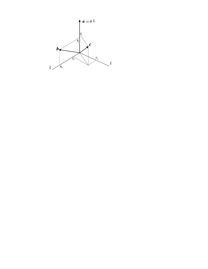
Figure 2: The vector representation of the matrix elements. The three lines in the Cholesky decomposition can be represented by three vectors: The coordinate system is chosen so that the vector $\vec{a}=a\hat{x}$ lies on the $x$-axis, while $\vec{b}$ lies on the $(x,y)$-plane.

Summarizing, we emphasize that once the physical properties of the triangular matrix have been explored, any other possible physically equivalent form (symmetric or non-symmetric texture) can be obtained by means of an orthogonal transformation which in standard parametrization reads

$$U=\left(\begin{array}[]{ccc}\cos\alpha\cos\gamma&\cos\gamma\sin\alpha&\sin\gamma\\ -\cos\beta\sin\alpha-\cos\alpha\sin\beta\sin\gamma&\cos\alpha\cos\beta-\sin\alpha\sin\beta\sin\gamma&\cos\gamma\sin\beta\\ \sin\alpha\sin\beta-\cos\alpha\cos\beta\sin\gamma&-\cos\alpha\sin\beta-\cos\beta\sin\alpha\sin\gamma&\cos\beta\cos\gamma\end{array}\right)$$ (78)

Indeed, since $\left\{M_{C}{\,U}\right\}\left\{{U\,}^{T}M_{C}^{T}\right\}=M_{C}M_{C}^{T}$, we can generate equivalent forms by means of the transformation $M_{x}=M_{C}{\,U}$ as already was proven above. Thus, the first line of $M_{x}$ for example becomes

$${M_{x}}_{1} = \{a_{1}\cos\alpha\cos\gamma,a_{1}\sin\alpha\cos\gamma,a_{1}\sin\gamma\}$$

while analogous, although more lengthy expressions hold for the other two lines too. We therefore see that the orthogonal matrix rearranges the elements within a given line of the mass matrix, but never mixes them with the elements of the other lines. Generally, if ${M_{x}}_{i}$ is the $i$-th line (or a three-component vector in our notation), then the inner product is ${M_{x}}_{i}{M_{x}}_{i}$ while the orthogonal transformation does not alter the magnitude of the vector, so

$${M_{x}}_{1}\cdot{M_{x}}_{1} = |\vec{a}|^{2}=a_{1}^{2}$$

$${M_{x}}_{2}\cdot{M_{x}}_{2} = |\vec{b}|^{2}=b_{1}^{2}+b_{2}^{2}$$ (79)

$${M_{x}}_{3}\cdot{M_{x}}_{3} = |\vec{c}|^{2}=c_{1}^{2}+c_{2}^{2}+c_{3}^{2}$$

Notice also that these quantities coincide with the diagonal elements of $M_{C}M_{C}^{T}$, which implies that

$$|\vec{a}|^{2}+|\vec{b}|^{2}+|\vec{c}|^{2}=m_{1}^{2}+m_{2}^{2}+m_{3}^{2}$$

Also, the product of the entries on the diagonal equals the product of the eigenmasses

$$a_{1}b_{2}c_{3}=m_{1}m_{2}m_{3}$$

For our purposes, the crucial observation here is that the magnitudes of the three vectors $\vec{a},\vec{b},\vec{c}$ which represent the three lines of the matrix, remained unaltered under the multiplication of $M_{C}$ by orthogonal transformations. Therefore, since any matrix can be cast in triangular form by an orthogonal transformation, we can concentrate our analysis in the latter. The peculiar form of the matrices derived in the previous section, where each line of mass entries is related to a different mass generating mechanism, justifies an analogous treatment.

Following the discussion above we attempt now to construct analytically $M_{C}$ from a general mass matrix and correlate its elements to those of the corresponding triangular form. This procedure essentially corresponds to the decomposition of a square matrix to its triangular form times an orthogonal matrix (QL decomposition). To this end, we consider the general $3\times 3$ mass matrix

$$m = \left(\begin{array}[]{ccc}m_{11}&m_{12}&m_{13}\\ m_{21}&m_{22}&m_{23}\\ m_{31}&m_{32}&m_{33}\end{array}\right)$$ (83)

Next we define the vectors $\vec{\xi}_{j}$, $j=1,2,3$

$$\vec{\xi}_{j} = (m_{j1},m_{j2},m_{j3})$$ (84)

hence, the matrix can be written

$$m = \left(\begin{array}[]{c}\vec{\xi}_{1}\\ \vec{\xi}_{2}\\ \vec{\xi}_{3}\end{array}\right)$$ (88)

To construct the Cholesky matrix we rely on the Gram-Schmidt orthogonalization procedure and introduce the following orthogonal set

$$\vec{u}_{i} = \vec{\xi}_{i}-\sum_{j=1}^{i-1}(\vec{\xi}_{i}\cdot\hat{e}_{j})\,\hat{e}_{j},\;i=1,2,3$$ (89)

where we have defined the following three orthogonal unit vectors

$$\hat{e}_{i} = \frac{\vec{u}_{i}}{|\vec{u}_{i}|},\;i=1,2,3$$ (90)

Using the above formulae we can decompose the original matrix as follows

$$\left(\begin{array}[]{c}\vec{\xi}_{1}\\ \vec{\xi}_{2}\\ \vec{\xi}_{3}\end{array}\right) = \left(\begin{array}[]{ccc}\vec{\xi}_{1}\cdot\hat{e}_{1}&0&0\\ \vec{\xi}_{2}\cdot\hat{e}_{1}&\vec{\xi}_{2}\cdot\hat{e}_{2}&0\\ \vec{\xi}_{3}\cdot\hat{e}_{1}&\vec{\xi}_{3}\cdot\hat{e}_{2}&\vec{\xi}_{3}\cdot\hat{e}_{3}\end{array}\right)\left(\begin{array}[]{c}\hat{e}_{1}\\ \hat{e}_{2}\\ \hat{e}_{3}\end{array}\right)$$ (100)

where the last column defines a orthogonal matrix

$$U = \left(\begin{array}[]{c}\hat{e}_{1}\\ \hat{e}_{2}\\ \hat{e}_{3}\end{array}\right)$$ (104)

whose elements are determined by (89) and (90). The formula (100) is an explicit realization of (68) with $U$ given by (104). Using this latter representation of the triangular matrix, in the next section we will give simple analytic formulae of its non-zero entries as functions of the mass eigenstates and the diagonalizing matrix elements.

4 The rotating matrices

We have seen that the triangular form of the mass matrix plays the rôle of the progenitor of all classes of symmetric as well as non-symmetric mass matrices with the same physical properties. Once the triangular form of the mass matrix is determined, its multiplication with an orthogonal mass matrix $U(\alpha,\beta,\gamma)$ leads to an equivalent texture which, depending on the specific choice of the angles $\alpha,\beta,\gamma$ of the $U$ matrix may be symmetric or non-symmetric or might have some simplified texture-zero form. All matrices obtained through this procedure from the same progenitor result to the symmetric product $mm^{T}$, thus they are characterized by the same diagonalizing orthogonal trasformation and the same eigevalues.

Therefore, the triangular matrix contains all the necessary information for the mixing and mass eigenstates. Its usefulness will be evinced by the fact that all its entries can be expressed as simple functions of the eigenmasses and the elements of the diagonalizing matrix. In the basis where one of the quark matrices is diagonal, all the elements of the other quark sector in its triangular form are uniquely determined in terms of the mass eigenstates and the CKM mixing. When up and down quark matrices appear in non-diagonal form, the elements of the triangular matrices are not uniquely determined. The entries of each matrix can be expressed in terms of the eigenmasses and the angles of the diagonalizing orthogonal matrix, whilst, only the elements of the product $V_{u}^{\dagger}V_{d}$ of the two transformations is constrained to be the CKM matrix. Therefore, as expected, a variety of mass textures can result to the known CKM mixing. The triangular form of the mass textures gives the advantage of treating in a simple and economical manner the problem of finding the admissible classes of quark matrices which reconcile the experimental data of mass and CKM mixing.

In this section we develop a general formalism to determine all possible classes of admissible mass textures for the up and down quark sectors. As pointed out, our procedure is general and applies equally well in the case of the lepton sector. We introduce here a novel parametrization of the orthogonal matrices and the CKM matrix which will facilitate the subsequent analysis. To this end, let us define the antisymmetric $3\times 3$ matrices

$$s_{1}=\begin{bmatrix}0&0&0\\ 0&0&1\\ 0&-1&0\end{bmatrix},\;\;s_{2}=\begin{bmatrix}0&0&1\\ 0&0&0\\ -1&0&0\end{bmatrix},\;\;s_{3}=\begin{bmatrix}0&1&0\\ -1&0&0\\ 0&0&0\end{bmatrix}\cdot$$ (105)

and a unit vector

$$\hat{n} = (n_{1},n_{2},n_{3})$$ (106)

Using the Cayley-Hamilton theorem [25], we find that the exponential of the $3\times 3$ matrices proportional to the inner product $\hat{n}\cdot\vec{s}$ is written

$$\exp\left[\alpha\widehat{n}\overrightarrow{s}\right]=1+\sin\alpha~{}\widehat{n}\cdot\overrightarrow{s}+\left(1-\cos\alpha\right)\left(\widehat{n}\cdot\overrightarrow{s}\right)^{2}$$ (107)

or equivalently

$$\exp\left[\alpha\widehat{n}\overrightarrow{s}\right]=1+\sin\alpha~{}\widehat{n}\cdot\overrightarrow{s}+2\sin^{2}\left(\frac{\alpha}{2}\right)\left(\widehat{n}\cdot\overrightarrow{s}\right)^{2}\cdot$$ (108)

The general orthogonal matrix can therefore be written as

$$U=\exp\left[\alpha\widehat{n}\cdot\overrightarrow{s}\right]$$ (109)

Indeed, since $\widehat{n}\cdot\overrightarrow{s}$ is traceless, the determinant of $U$ is unity and since $\widehat{n}\cdot\overrightarrow{s}$ is antisymmetric it ensures that $U^{T}U=1$. Therefore, the orthogonal matrix can be parametrized by the angle $\alpha$ and the unit vector $\hat{n}$ whose components constitute the directional cosines along the ‘directions’ $s_{1,2,3}$.

To get a feeling of this new parametrization in terms of the ‘orthogonal’ basis $s_{1},s_{2},s_{3}$ of the orthogonal matrix and its correlation with the standard parametrization, let us consider the particular case where the vector $\hat{n}$ is aligned along a specific ‘axis’, i.e. let $\hat{n}=(0,0,1)$. Then

$$U(\alpha) = \exp\left[\alpha\,{s_{3}}\right]\equiv\left(\begin{array}[]{lll}\cos(\alpha)&\sin(\alpha)&0\\ -\sin(\alpha)&\cos(\alpha)&0\\ 0&0&1\end{array}\right)$$ (113)

Analogous expressions hold for alignments to the remaining two axes.

For our subsequent analysis it is also useful to express the CKM matrix in the basis $s_{1},s_{2},s_{3}$. Plugging in the numerical values of its entries as they are measured by the experiment (see appendix) we find that the CKM matrix can be written

$$V_{CKM}=\exp[\phi_{c}\widehat{n}\overrightarrow{s}]$$ (114)

where the angle $\phi_{c}=0.231505$ and the unit vector components along the orthogonal directions $s_{1},s_{2},s_{3}$ are

$$\widehat{n}=\begin{bmatrix}0.179694\\ 0.0177102\\ 0.983564\end{bmatrix}$$ (115)

This result shows that the CKM matrix is predominantly a rotation around the third axis $s_{3}$. Since $V_{CKM}=V_{u}^{\dagger}V_{d}$ the combined effect of the up and down rotation matrices should produce a rotation mostly around the third axis. In principle, for any choice of $V_{d}$ there is always a $V_{u}$ orthogonal matrix that is consistent with $V_{CKM}$, however we will see that the observed quark mass hierarchy will reduce substantially these choices.

Our objective is to find the conditions on D-brane inspired mass matrices so that they are consistent with the experimental data. Thus, given the CKM mixing and the predicted form of the down (up) quark mass texture, we will use the above analysis to determine the form of the corresponding up (down) quark matrix. Starting for example with the down quark mass matrix, and the orthogonal matrix $V_{d}$ which diagonalizes the down quarks, then we need in this new formalism a convenient way to express the diagonalizing matrix of the up quarks which is given by $V_{u}=V_{d}V_{CKM}^{\dagger}$. To express in a simple way the multiplication of two arbitrary orthogonal matrices, we use the formula (109). Obviously, the resulting matrix is also orthogonal, therefore it can be expressed in terms of a new unit vector and a new angle. If we identify $\hat{a}$ with the unit vector related to the diagonalizing matrix of the up-quarks and $\hat{b}$ with the unit vector associated to the corresponding one for the down quarks, we can apply directly the Cayley-Hamilton formula for the multiplication $V_{u}=V_{d}V_{CKM}^{\dagger}$, to obtain

$$\hat{a} = \frac{1}{\sin\frac{\alpha}{2}}\left\{\sin\frac{\beta}{2}\cos\frac{\phi_{c}}{2}\,\hat{b}-\cos\frac{\beta}{2}\,\sin\frac{\phi_{c}}{2}\,\hat{n}-\sin\frac{\phi_{c}}{2}\,\sin\frac{\beta}{2}\,\hat{b}\times\hat{n}\right\}$$ (116)

The angles are also related by the additional expression

$$\cos\frac{\phi_{c}}{2} = \cos\frac{\alpha}{2}\cos\frac{\beta}{2}+\sin\frac{\alpha}{2}\,\sin\frac{\beta}{2}\cos\theta$$ (117)

where $\cos\theta=\hat{a}\cdot\hat{b}$, thus the CKM angle $\phi_{c}$ is directly expressed in terms of the relative declination of the ‘rotational’ axes of the down and up quark diagonalizing matrices.

Let’s see two limiting cases that will be useful in our subsequent examples: If we choose $\hat{b}$ to be aligned with the CKM-axis $\hat{b}=\hat{n}$ , then $\hat{b}\times\hat{n}=0$ and $\hat{a}$ is given as a combination of the two remaining components on the RHS of (116)

$$\sin\frac{\alpha}{2}\,\hat{a}=\left(\sin\frac{\beta}{2}\cos\frac{\phi_{c}}{2}-\cos\frac{\beta}{2}\,\sin\frac{\phi_{c}}{2}\right)\,\hat{n}$$

This is satisfied if $\hat{a}=\pm\hat{n}$, and

$$\pm\sin\frac{\alpha}{2}=\sin\frac{\beta-\phi_{c}}{2}$$

i.e., if $\beta-\alpha=2k\,\pi+\phi_{c}$. Choosing $\hat{b}=-\hat{n}$, we find $\alpha-\beta=2k\,\pi+\phi_{c}$.

A second limiting case arises if we choose $\vec{a}\cdot\vec{b}=0$. Then $\cos\theta=0$ and the three angles are related by the simple expression

$$\cos\frac{\phi_{c}}{2}=\cos\frac{\alpha}{2}\,\cos\frac{\beta}{2}.$$

Before closing this section, let us point out for later convenience that the formula (116) can be expressed in a more compact form. Indeed, if we redefine

$$\hat{a} \rightarrow \vec{a}=\hat{a}\sin\frac{\alpha}{2}$$

$$\hat{b} \rightarrow \vec{b}=\hat{b}\sin\frac{\beta}{2}$$

and

$$\hat{n} \rightarrow \vec{c}=\hat{n}\sin\frac{\phi_{c}}{2}$$ (118)

we rewrite (116) in the following simplified expression

$$\vec{a} = \cos\frac{\phi_{c}}{2}\,\vec{b}-\cos\frac{\beta}{2}\,\vec{c}-\vec{b}\times\vec{c}$$ (119)

5 Analytic expressions

In our previous examples of mass matrices emerging in effective models from consistent D-brane configurations, we have seen that novel fermion mass textures appear where their entries do not exhibit the expected ‘hierarchical’ pattern.

In fact, for the cases presented previously the mass entries of a certain line of the mass matrix emerge from a certain source, thus, each line is characterized by a certain mass scale which in general differs from the scale of another line. Clearly, this scale should be correlated to some appropriate (eventually invariant under some specific operation) quantity and not to a single coupling which might be accidentally zero due to some particular choice of the basis. In this case in our subsequent analysis it is adequate to deal mainly with the magnitudes of the vectors $\vec{\xi}_{j}^{u,d}$, $j=1,2,3$, or equivalently the magnitudes of the lines of the corresponding triangular matrix (100).

We can determine all possible acceptable mass textures if we express the elements of the corresponding triangular mass matrices only as functions of the directional cosines and the mass eigenvalues, i.e., the masses of the quarks.

To proceed further we recall from the analysis of the previous sections that for a given (in general) non-symmetric matrix $m$, it holds $mm^{T}=M_{C}M_{C}^{T}$, where $M_{C}$ is the Cholesky from. In the present section we give analytic formulae for the triangular form $M_{C}$ with its entries expressed only in terms of the eigenmasses of $mm^{T}$ and the elements of its diagonalizing orthogonal matrix. Let us start with the evaluation of the entries of the orthogonal transformation. Assuming the orthogonal transformation $U(\alpha)$ given by the Cayley-Hamilton formula while redefining

$$\widehat{a}\rightarrow\sin\frac{\alpha}{2}\,\vec{a}~{}\cdot$$ (120)

we get the following simplified expression for the orthogonal matrix

$$U(\alpha)=1+2\cos\frac{\alpha}{2}\overrightarrow{a}\cdot\overrightarrow{s}+2\left(\overrightarrow{a}\cdot\overrightarrow{s}\right)^{2}$$ (121)

where now the vector $\vec{a}$ is no logger a unit vector,

$$\overrightarrow{a}^{2} = a_{1}^{2}+a_{2}^{2}+a_{3}^{2}=\sin^{2}\frac{\alpha}{2}$$ (122)

It is useful to write the orthogonal matrix in expanded form. We get

$$U({\alpha})=\begin{bmatrix}\cos\alpha+2a_{1}^{2}&2\left(a_{3}\cos\frac{\alpha}{2}-a_{1}a_{2}\right)&2\left(a_{2}\cos\frac{\alpha}{2}+a_{1}a_{3}\right)\\ -2\left(a_{3}\cos\frac{\alpha}{2}+a_{1}a_{2}\right)&\cos\alpha+2a_{2}^{2}&2\left(a_{1}\cos\frac{\alpha}{2}-a_{2}a_{3}\right)\\ -2\left(a_{2}\cos\frac{\alpha}{2}-a_{1}a_{3}\right)&-2\left(a_{1}\cos\frac{\alpha}{2}+a_{2}a_{3}\right)&\cos\alpha+2a_{3}^{2}\end{bmatrix}$$ (123)

where $a_{1,2,3}$ are not all independent since they satisfy (122). Therefore, $U(\alpha)$ is expressed only in terms of three independent parameters as expected. We can now express analytically the elements of the triangular matrix as functions of the orthogonal matrix entries $u_{ij}$ and the mass eigenstates as follows

$$\overrightarrow{\xi}_{1}\cdot\overrightarrow{e}_{1} = \sqrt{u_{11}^{2}m_{1}^{2}+u_{12}^{2}m_{2}^{2}+u_{13}^{2}m_{3}^{2}}$$

$$\overrightarrow{\xi}_{2}\cdot\overrightarrow{e}_{2} = \sqrt{\frac{u_{33}^{2}m_{1}^{2}m_{2}^{2}+u_{31}^{2}m_{2}^{2}m_{3}^{2}+u_{32}^{2}m_{1}^{2}m_{3}^{2}}{u_{11}^{2}m_{1}^{2}+u_{12}^{2}m_{2}^{2}+u_{13}^{2}m_{3}^{2}}}$$

$$\overrightarrow{\xi}_{3}\cdot\overrightarrow{e}_{3} = \frac{m_{1}m_{2}m_{3}}{\sqrt{u_{33}^{2}m_{1}^{2}m_{2}^{2}+u_{31}^{2}m_{2}^{2}m_{3}^{2}+u_{32}^{2}m_{1}^{2}m_{3}^{2}}}$$

$$\overrightarrow{\xi}_{2}\cdot\overrightarrow{e}_{1} = \frac{u_{11}u_{21}m_{1}^{2}+u_{22}u_{12}m_{2}^{2}+u_{13}u_{23}m_{3}^{2}}{\sqrt{u_{11}^{2}m_{1}^{2}+u_{12}^{2}m_{2}^{2}+u_{13}^{2}m_{3}^{2}}}$$ (124)

$$\overrightarrow{\xi}_{3}\cdot\overrightarrow{e}_{1} = \frac{u_{11}u_{31}m_{1}^{2}+u_{32}u_{12}m_{2}^{2}+u_{33}u_{13}m_{3}^{2}}{\sqrt{u_{11}^{2}m_{1}^{2}+u_{12}^{2}m_{2}^{2}+u_{13}^{2}m_{3}^{2}}}$$

$$\overrightarrow{\xi}_{3}\cdot\overrightarrow{e}_{2} = -\frac{u_{23}u_{33}m_{1}^{2}m_{2}^{2}+u_{21}u_{31}m_{2}^{2}m_{3}^{2}+u_{22}u_{32}m_{1}^{2}m_{3}^{2}}{\sqrt{u_{11}^{2}m_{1}^{2}+u_{12}^{2}m_{2}^{2}+u_{13}^{2}m_{3}^{2}}\sqrt{u_{33}^{2}m_{1}^{2}m_{2}^{2}+u_{31}^{2}m_{2}^{2}m_{3}^{2}+u_{32}^{2}m_{1}^{2}m_{3}^{2}}}~{}.$$

Thus, the triangular matrix elements are simple functions of the eigenmasses and the orthogonal transformation entries. This analytic result simplifies remarkably the analysis of classifying experimentally admissible mass matrices, while we note that several simple textures can be found even by simple inspection of the above analytic structure.

We can use an alternative parametrization of the triangular matrix reliant on the relations (124) as follows. We define the diagonal matrix of the squared mass eigenvalues

$${\cal M} = \left(\begin{array}[]{ccc}m_{1}^{2}&0&0\\ 0&m_{2}^{2}&0\\ 0&0&m_{3}^{2}\end{array}\right)$$ (128)

and the vectors

$$\vec{v}_{i} = (u_{i1},u_{i2},u_{i3})$$ (129)

where $u_{ij}$ are the elements of the diagonalizing matrix, thus $\vec{v}_{i}\cdot\vec{v}_{j}=\delta_{ij}$. In this notation, the nominator of the $\{21\}$ entry of the triangular matrix is written

$$\vec{\xi}_{2}\cdot\hat{e}_{1} \propto \vec{v}_{2}{\cal M}\vec{v}_{1}\;\equiv\;\vec{v}_{1}{\cal M}\vec{v}_{2}=\sum_{i=1}^{3}u_{2i}m_{i}^{2}u_{1i}$$ (130)

Similarly, we find also also that the $\{31\}$ entry is proportional to

$$\vec{\xi}_{3}\cdot\hat{e}_{1} \propto \vec{v}_{3}{\cal M}\vec{v}_{1}\;\equiv\;\vec{v}_{1}{\cal M}\vec{v}_{3}=\sum_{i=1}^{3}u_{3i}m_{i}^{2}u_{1i}$$ (131)

and the $\{32\}$

$$\vec{\xi}_{3}\cdot\hat{e}_{2} \propto \vec{v}_{3}{\cal M}^{-1}\vec{v}_{2}\;\equiv\;\vec{v}_{2}{\cal M}\vec{v}_{3}=\sum_{i=1}^{3}u_{3i}m_{i}^{-2}u_{2i}$$ (132)

In this notation, all entries are expressed in terms of inner products $\vec{v}_{j}{\cal M}^{n}\vec{v}_{i}$, $n={\pm 1}$, and the triangular mass matrix takes the following elegant form

$$M_{C} = \left(\begin{array}[]{ccc}\sqrt{\vec{v}_{1}{\cal M}\vec{v}_{1}}&0&0\\ \frac{\vec{v}_{2}{\cal M}\vec{v}_{1}}{\sqrt{\vec{v}_{1}{\cal M}\vec{v}_{1}}}&\sqrt{\frac{\vec{v}_{3}{\cal M}^{-1}\vec{v}_{3}}{\vec{v}_{1}{\cal M}\vec{v}_{1}}}\,m_{1}m_{2}m_{3}&0\\ \frac{\vec{v}_{3}{\cal M}\vec{v}_{1}}{\sqrt{\vec{v}_{1}{\cal M}\vec{v}_{1}}}&-\frac{\vec{v}_{3}{\cal M}^{-1}\vec{v}_{1}\,m_{1}m_{2}m_{3}}{\sqrt{(\vec{v}_{1}{\cal M}\vec{v}_{1})(\vec{v}_{3}{\cal M}^{-1}\vec{v}_{3})}}&\frac{1}{\sqrt{\vec{v}_{3}{\cal M}^{-1}\vec{v}_{3}}}\\ \end{array}\right)$$ (136)

The form (136) of the triangular matrix will prove particularly useful for the classification of the textures with zeroes discussed in the subsequent sections.

5.1 Mass textures with zeroes

In phenomenological investigations, a usual practice to minimize the number of arbitrary mass parameters to those which suffice to determine the quark mass eigenstates, is to seek viable texture-zero mass matrices. In this section we are going to explore in detail this issue motivated also by the fact that in several cases of String and D-brane models, negligible or even zero entries in Yukawa textures do persist even after the inclusion of non-renormalizable or other contributions, because of remnant discrete or other symmetries left over from the higher theory. This is also the case in F-theory constructions when some matter fields are localized on different curves [17].

The analytic result obtained above for the Cholesky form of a matrix allows the classification of texture-zero mass matrices in a simple and elegant way. We first note that the Cholesky form of the matrix is already a non-symmetric texture-zeroes Yukawa matrix itself. Using suitable values for the angles $(\alpha,\beta,\gamma)$ of the orthogonal transformation (78) we can obtain more texture-zero forms of the mass matrix $m_{D}$. Up to possible signs, while without assuming any further relation of the diagonalizing matrix and the mass matrix entries, we find that in addition to (100) there are only four more non-symmetric texture zero forms, namely

$$\left(\begin{array}[]{ccc}0&0&a_{1}\\ 0&-b_{2}&b_{1}\\ c_{3}&-c_{2}&c_{1}\end{array}\right) \left(\begin{array}[]{ccc}0&0&a_{1}\\ -b_{2}&0&b_{1}\\ -c_{2}&-c_{3}&c_{1}\end{array}\right)$$ , (143)

$$\left(\begin{array}[]{ccc}0&a_{1}&0\\ 0&b_{1}&b_{2}\\ c_{3}&c_{1}&c_{2}\end{array}\right) \left(\begin{array}[]{ccc}0&a_{1}&0\\ -b_{2}&b_{1}&0\\ -c_{2}&c_{1}&c_{3}\end{array}\right)$$ , (150)

These essentially correspond to simple rearrangements of the zeroes of the initial matrix under trivial transformations.

A less trivial and more appealing task is of course to minimize further the arbitrary parameters of (100) by setting additional entries equal to zero yet reconciling the experimental data. To this end, we proceed to a classification of all non-trivial zeroes of the down-quark mass matrix setting successively in (124) the off-diagonal elements equal to zero, i.e. $\vec{\xi}_{j}\cdot\hat{e}_{i}=0$, and derive the conditions implied for the remaining non-zero matrix elements. Having determined the specific forms of $m_{D}$, we can use the results of each individual solution to determine the corresponding up quark texture. We first start with the observation that none of the three diagonal elements of the triangular matrix can be set equal to zero since this would imply that at least one eigenmass is zero which contradicts the data. Therefore, the only possible zeroes in a Cholesky matrix can be found in the off-diagonal entries $\{21\},\{31\},\{32\}$.

5.1.1 The case of one diagonal quark mass matrix

We start with the simplest (trivial) possibility where all possible entries in the down-quark Cholesky mass matrix are zero, i.e. a texture three-zeroes,

$$m_{D_{21}}=m_{D_{31}}=m_{D_{32}}=0$$

This implies that the down quark mass matrix is in diagonal form, therefore its diagonalizing matrix is the identity matrix $V_{d}=I$, whilst $V_{u}=V_{CKM}^{\dagger}$. Therefore the up-quark mass diagonalizing orthogonal matrix has the form (100), its elements being $u_{ij}=\left(V_{CKM}^{\dagger}\right)_{ij}$. Substituting the appropriate experimental values of masses and mixing, the numerical form of the matrix is

$${m_{U}} \approx \left(\begin{array}[]{lll}0.293&0&0\\ -3.792&6.150&0\\ 64.938&-158.029&0.342\end{array}\right)$$ (154)

with all entries expressed in GeV. It is easy to see that the square roots of the eigenvalues of the matrix $m_{U}m_{U}^{T}$ are the up quark masses $m_{u}=0.003,m_{c}=1.21,m_{t}=171$GeV as expected. Thus, in the basis where the down quark mass matrix is diagonal, all entries of the up-quark mass matrix are non-zero, whilst the line-vectors $\vec{\xi}_{j}^{u}$ (in the notation (88) of the matrix $m_{U}$) exhibit a hierarchical pattern  in the sense that $|\vec{\xi}_{1}^{u}|<|\vec{\xi}_{2}^{u}|<|\vec{\xi}_{3}^{u}|$ and this is true for a whole class of equivalent matrices which are obtained when orthogonal transformations are acting on the progenitor from the right. Indeed, multiplying by any orthogonal matrix from the RHS, the measures of the vectors $|\vec{\xi}_{j}|$ do not change. For example, acting with an orthogonal transformation the first vector $\vec{\xi}_{1}$ becomes

$$\vec{\xi}^{\prime}_{1}=\{1.52781\cos(\alpha)\cos(\gamma),1.52781\cos(\gamma)\sin(\alpha),1.52781\sin(\gamma)\}$$ (155)

while it can be checked that $|\vec{\xi}_{1}|=|\vec{\xi}^{\prime}_{1}|$ and in the same manner $|\vec{\xi}_{2,3}|=|\vec{\xi}^{\prime}_{2,3}|$. Thus, if the down quark mass matrix is cast to diagonal form, the mass hierarchy and CKM imply definite hierarchical structure

$$|\vec{\xi}_{1}|\,:\,|\vec{\xi}_{2}|\,:\,|\vec{\xi}_{3}|\,\sim\,\rho^{4}\,:\,\rho^{2}\,:\,1$$

with $\rho\sim 0.2$. We will see in the next sections that the hierarchy of the vectors $|\vec{\xi}_{i}|$ can be reversed if both matrices are non-diagonal but in limited regions of the parameter space in order to achieve consistency with the CKM mixing.

5.1.2 Textures with two-zeros

We turn now to the non-trivial texture-zero cases with non-diagonal mass matrices. We demand that the entry $\{21\}$ is zero, thus we take $\vec{\xi}_{2}\cdot\hat{e}_{1}=0$ which implies

$$u_{11}u_{21}m_{1}^{2}+u_{22}u_{12}m_{2}^{2}+u_{13}u_{23}m_{3}^{2} = 0$$ (156)

We first try to satisfy the above condition without assuming a particular relation between $u_{ij}$ and the mass eigenvalues $m_{i}$. Two possible solutions are

$$i) u_{12}=u_{21}=u_{13}=0\;{\rm or}$$ (157)

$$ii) u_{12}=u_{21}=u_{23}=0$$ (158)

Starting with the first case, from $u_{12}=u_{21}=0$ it follows from (123)

$$a_{3}\cos\frac{\alpha}{2}\pm a_{1}a_{2}=0$$

A)  A simple (although not the only) way to satisfy the above is by choosing $a_{2}=a_{3}=0$, so that $a_{1}=\sin\frac{\alpha}{2}$ and the diagonalizing and Cholesky matrices assume the simplified form

$$U_{a}=\left(\begin{array}[]{ccc}1&0&0\\ 0&\cos\,\alpha&\sin\,\alpha\\ 0&-\sin\,\alpha&\cos\,\alpha\end{array}\right) M_{C}=\left(\begin{array}[]{ccc}x_{11}&0&0\\ 0&x_{22}&0\\ 0&x_{32}&x_{33}\end{array}\right)$$ (165)

with $x_{11}=m_{1}$, $x_{22}=\pm\sqrt{m_{3}^{2}-\delta_{32}^{2}\cos^{2}\alpha},\,x_{33}=m_{2}m_{3}/x_{22}$, and $x_{32}=\delta_{32}^{2}\sin(2\alpha)/(2x_{22})$, where $\delta_{ji}^{2}=(m_{j}^{2}-m_{i}^{2})$.

B)  If we take the second case, then $a_{1}=a_{3}=0$, so that $a_{2}=\sin\frac{\alpha}{2}$ and the matrices are reduced to

$$U_{a}=\left(\begin{array}[]{ccc}\cos\,\alpha&0&\sin\,\alpha\\ 0&1&0\\ -\sin\,\alpha&0&\cos\,\alpha\end{array}\right) M_{C}=\left(\begin{array}[]{ccc}x_{11}&0&0\\ 0&x_{22}&0\\ x_{31}&0&x_{33}\end{array}\right)$$ (172)

with $x_{11}=\sqrt{m_{3}^{2}-\delta_{31}^{2}\cos^{2}\alpha},x_{22}=m_{2},x_{33}=m_{1}m_{3}/x_{11}$, and $x_{31}=\delta_{31}^{2}\sin(2\alpha)/(2x_{11})$.

C)  Next we assume that $\vec{\xi}_{3}\cdot\hat{e}_{1}=0$. This implies one new case, $a_{1}=a_{2}=0$ and the following structure

$$U_{a}=\left(\begin{array}[]{ccc}\cos\,\alpha&\sin\,\alpha&0\\ -\sin\,\alpha&\cos\,\alpha&0\\ 0&0&1\end{array}\right) M_{C}=\left(\begin{array}[]{ccc}x_{11}&0&0\\ x_{21}&x_{22}&0\\ 0&0&x_{33}\end{array}\right)$$ (179)

with $x_{11}=m_{2}^{2}-\delta_{21}^{2}\cos\alpha$, $x_{22}=\pm m_{1}m_{2}/x_{11},x_{33}=m_{3}$ and $x_{21}=\delta_{21}^{2}\sin(2\alpha)/(2x_{11})$.

A thorough and rigorous analysis of the textures with two-zeroes is presented in detail in the appendix. It is shown that all other possible solutions can be reduced to the above three cases by trivial transformations. We observe that when no specific relation between the eigenvalues $m_{i}$ and the mixing entries $u_{ij}$ is assumed, the triangular matrix cannot have a single zero off-diagonal element. There are always two zeroes in the triangular matrix which are always correlated to one of the three angles in the diagonalizing matrix (78).

For any of the above cases we can now compute the diagonalizing up-quark orthogonal matrix and use this result to calculate the entries of the corresponding up quark mass matrix. All elements of the two triangular matrices can be expressed in terms of one free parameter, namely the angle $\alpha$. In deploying our procedure in the next subsection we are going to use this freedom to pin down quark mass patterns, in particular those which can be in accordance with specific classes from D-brane configurations.

5.1.3 Textures with one zero

The case of triangular matrices with only one zero element is more involved. We have seen in the previous subsection that whenever we demand one of the entries to be zero, there is always a second zero element in the matrix unless a non-trivial relation between $u_{ij}$ and the mass eigenstates $m_{i}$ is imposed. In the following, we will derive and discuss in detail these conditions for the case that the only zero is $\vec{\xi}_{2}\cdot\hat{e}_{1}=0$. The analysis can be easily extended to the other two non-diagonal elements of the triangular matrix and for completeness is presented in the appendix. To proceed, we use the vector-like formalism of the triangular matrix elements introduced in (136). Then, the $\{21\}$ entry of the triangular matrix is proportional to

$$\vec{\xi}_{2}\cdot\hat{e}_{1} \propto \vec{v}_{2}{\cal M}\vec{v}_{1}\;\equiv\;\vec{v}_{1}{\cal M}\vec{v}_{2}=\sum_{i=1}^{3}u_{2i}m_{i}^{2}u_{1i}$$ (180)

The requirement that the $\{21\}$ element in the mass matrix is equal to zero, is now equivalent to the orthogonality condition

$$\vec{v}_{2}{\cal M}\vec{v}_{1}=\vec{v}_{1}{\cal M}\vec{v}_{2}=0$$

The condition $\vec{v}_{2}{\cal M}\vec{v}_{1}=0$ implies that the vector ${\cal M}\vec{v}_{1}$ is orthogonal to $\vec{v}_{2}$ and therefore can be expressed as a linear combination of $\vec{v}_{1},\vec{v}_{3}$. Similarly $\vec{v}_{1}{\cal M}\vec{v}_{2}=0$ implies that ${\cal M}\vec{v}_{2}$ can be expressed in terms of $\vec{v}_{2},\vec{v}_{3}$. We find

$${\cal M}\vec{v}_{1} = \left(\vec{v}_{1}{\cal M}\vec{v}_{1}\right)\,\vec{v}_{1}+\left(\vec{v}_{3}{\cal M}\vec{v}_{1}\right)\,\vec{v}_{3}$$

$${\cal M}\vec{v}_{2} = \left(\vec{v}_{2}{\cal M}\vec{v}_{2}\right)\,\vec{v}_{2}+\left(\vec{v}_{3}{\cal M}\vec{v}_{2}\right)\,\vec{v}_{3}$$

Both of the above can be solved for $\vec{v}_{3}$, giving

$$\vec{v}_{3} = \frac{1}{\left(\vec{v}_{3}{\cal M}\vec{v}_{k}\right)}\left({\cal M}-\vec{v}_{k}{\cal M}\vec{v}_{k}\right)\,\vec{v}_{k},\;k=1{\rm or}\;2$$ (181)

or, in component form ($A_{ji}=\vec{v}_{j}{\cal M}\vec{v}_{i}=\sum_{i=1}^{3}u_{jl}m_{l}^{2}u_{il}$)

$$u_{3j} = \frac{m_{j}^{2}-A_{kk}}{A_{3k}}\,u_{kj},\;k=1,2,\;j=1,2,3$$ (182)

Thus, the relations (182) are sufficient to ensure that at least the $\{21\}$ element of the triangular mass matrix is zero, while similar relations hold for the vanishing of the other off-diagonal elements. By simple inspection of the above formula we find that if some $u_{kj}$ on the right-hand side of (182) is set equal to zero, then the two-zeroes textures discussed previously are recovered. Indeed, to make clear the argument, let us explore a particular case setting $u_{13}=0$. Putting $k=1$ in the above, we find that this implies $u_{33}=0$, while due to $u_{13}^{2}+u_{23}^{2}+u_{33}^{2}=1$ we get $u_{23}=1$. Putting $k=2$, we get

$$(m_{3}^{2}-A_{22})\,u_{23} = 0$$

Since $u_{23}$ is non-zero, ($u_{23}=1),$ we get

$$m_{3}^{2} = A_{22}=u_{21}^{2}m_{1}^{2}+u_{22}^{2}m_{2}^{2}+u_{23}^{2}m_{3}^{2}$$ (183)

which imposes the additional condition

$$u_{21}^{2}m_{1}^{2}+u_{22}^{2}m_{2}^{2} = 0$$

i.e., $u_{21}=u_{22}=0$. We further find $\vec{\xi}_{3}\cdot\hat{e}_{2}=0$, thus this case is reduced to textures with two-zeroes.

In the same way, we can prove that if any of the elements $u_{ki}$, $k=1,2,i=1,2,3$ is set equal to zero, we arrive at one of the textures with two-zeroes discussed previously.

Therefore, distinct, texture zero-one cases are possible only when all $u_{kj}\neq 0$, with $k$ taking the values 1 or 2 as above. This of course does not exclude that some of the remaining entries $u_{3j}$ could not be zero. In the next section we will present one such simple example of one zero texture mass matrix which is also compatible with D-brane patterns discussed in section 3.

5.2 On the relation with the symmetric texture-zero matrices

It is worth exploring the connection of the above triangular texture-zero analysis with the symmetric texture-zeroes already discussed in the literature sometime ago [8]. Using the mathematical analysis presented in previous section, it is straightforward to bring the latter into their corresponding triangular form. This calculation shows that from the set of the five texture zero symmetric mass matrices only one pair can be identified with a two-zeroes texture and one more with a the one-zero texture of our analysis. In particular, we find the following texture-zero triangular form

$$m_{U}=\begin{bmatrix}\varepsilon^{6}&0&0\\ 0&\varepsilon^{2}\sqrt{1+\varepsilon^{8}}&0\\ \varepsilon^{2}&\frac{1}{\sqrt{1+\varepsilon^{8}}}&\frac{\varepsilon^{4}}{\sqrt{1+\varepsilon^{8}}}\end{bmatrix},m_{D}=\begin{bmatrix}2\varepsilon^{4}&0&0\\ 2\varepsilon^{3}&2\varepsilon^{3}\sqrt{1+\varepsilon^{2}}&0\\ 2\varepsilon^{3}&\frac{1}{\sqrt{1+\varepsilon^{2}}}&\frac{\varepsilon}{\sqrt{1+\varepsilon^{2}}}\end{bmatrix}$$ (184)

which can be easily converted to one of the symmetric textures using the analysis of section 2.

The remaining three textures of  [8] -from the point of view of their progenitors- correspond to the general form with non-zero off-diagonal entries and the zeroes appear only in a certain point of the parameter space. To make this point clear, let us define the following triangular mass matrix for the down quarks

$$m_{D} = \left(\begin{array}[]{lll}2\epsilon^{4}&0&0\\ 2\epsilon^{3}&2\epsilon^{3}\sqrt{\epsilon^{2}+4}&0\\ 4\epsilon^{3}&\frac{2}{\sqrt{\epsilon^{2}+4}}&\frac{\epsilon}{\sqrt{\epsilon^{2}+4}}\end{array}\right)$$ (188)

Diagonalizing the symmetric $m_{D}m_{D}^{T}$, while choosing $\epsilon\sim.23$, we find the mass eigenvalues in good agreement with the values $m_{d},m_{s},m_{b}$. According to our discussion, there is an equivalent class of mass matrices obtained by the following $U$-action on $m_{D}$, $m_{D}\,U$, where $U$ is any orthogonal matrix. If we restrict to the orthogonal matrices, $U$ this is given by (78), thus the parameter space is defined by the angles $\alpha,\beta,\gamma$. Making the particular choice

$$\alpha_{0}=\frac{\pi}{2},\beta_{0}=\cos^{-1}\left(-\frac{\epsilon}{\sqrt{\epsilon^{2}+4}}\right),\gamma_{0}=0$$ (189)

we construct the equivalent symmetric texture-zero form

$$M_{D}=m_{D}\,{U}(\alpha_{0},\beta_{0},\gamma_{0})=\left(\begin{array}[]{ccc}0&2\epsilon^{4}&0\\ 2\epsilon^{4}&2\epsilon^{3}&4\epsilon^{3}\\ 0&4\epsilon^{3}&1\end{array}\right)$$ (193)

which is one of the texture-zeroes down quark mass matrices proposed in [8]. Therefore, the zeroes in (193) are completely accidental and arise due to the particular choice (189). An infinite number of equivalent mass matrices implies the same ‘physical’ quantities, namely the mass eigenstates and the diagonalizing matrix. For completeness, we give in the appendix the triangular form of the remaining four texture-zero symmetric quark mass matrices.

6 Examples of Admissible D-brane textures

Our present analysis has been motivated by the peculiar patterns of mass matrices which have appeared in certain D-brane configurations accommodating the Standard Model gauge symmetry. In this section, we will give simple examples where some of these D-brane inspired textures can appear, at least in some regions of the parameter space. Of course, the possibilities of finding consistent textures do increase if we assume the most general triangular mass matrices without imposing the rather restrictive conditions for zeroes. However, a complete analysis is beyond the scope of this paper. Instead, our aim is to illustrate how the new formalism applies in representative examples. We will concentrate in the case of texture-zero triangular forms and try to find some of the D-brane inspired textures that reconcile the experimental data.

6.1 The two-zeroes case

Once we have determined the texture with two-zeroes and the diagonalizing matrix of the down quarks, we can use the relations given in the previous section to construct the corresponding up quark mass texture. As an example of the method, we start with the down quark matrix such that the rotation is around the first axis, so the vector is $\vec{b}=(b_{1},0,0)$, with $b_{1}=\sin\frac{\beta}{2}$. The diagonalizing matrix is

$$\left(\begin{array}[]{ccc}1&0&0\\ 0&\cos\beta&\sin\beta\\ 0&-\sin\beta&\cos\beta\end{array}\right)$$ (197)

and the down quark matrix is found to be

$$m_{D} = \left(\begin{array}[]{ccc}m_{d}&0&0\\ 0&\sqrt{m_{s}^{2}\cos^{2}\beta+m_{b}^{2}\sin^{2}\beta}&0\\ 0&\frac{(m_{b}^{2}-m_{s}^{2})\sin(2\beta)}{2\sqrt{m_{s}^{2}\cos^{2}\beta+m_{b}^{2}\sin^{2}\beta}}&\frac{m_{b}m_{s}}{\sqrt{m_{s}^{2}\cos^{2}\beta+m_{b}^{2}\sin^{2}\beta}}\end{array}\right)$$ (201)

i.e., a two-zeroes triangular texture as expected. Using (119) we can determine the vector components of the diagonalizing matrix $V_{u}$

$$a_{1} = -\cos\frac{\beta}{2}\,c_{1}+\cos\frac{\phi_{c}}{2}\,\sin\frac{\beta}{2}$$ (202)

$$a_{2} = -\cos\frac{\beta}{2}\,c_{2}+\sin\frac{\beta}{2}\,c_{3}$$ (203)

$$a_{3} = -\cos\frac{\beta}{2}\,c_{3}-\sin\frac{\beta}{2}\,c_{2}$$ (204)

where the numerical values of the components $c_{i},i=1,2,3$ are calculated using (118) and (115). First, we consider the particular case where the up-quark mass matrix is rotated on the orthogonal direction, i.e., we demand the vector $\vec{a}$ to take the form $\vec{a}=(0,a_{2},a_{3})$. Imposing $a_{1}=0$ while using (119) we find

$$\tan\frac{\beta}{2} = +\frac{c_{1}}{\cos\frac{\phi_{c}}{2}}\equiv n_{1}\,\tan\frac{\phi_{c}}{2}$$ (205)

$$a_{2} = -\frac{\cos\frac{\beta}{2}}{\cos\frac{\phi_{c}}{2}}\,\left\{c_{2}\cos\frac{\phi_{c}}{2}-c_{1}c_{3}\right\}$$ (206)

$$a_{3} = -\frac{\cos\frac{\beta}{2}}{\cos\frac{\phi_{c}}{2}}\,\left\{c_{3}\cos\frac{\phi_{c}}{2}+c_{1}c_{2}\right\}$$ (207)

The angle entering the up-quark diagonalizing matrix is also fixed in this case and given by

$$\sin\frac{\alpha}{2} = \sqrt{\sin^{2}\frac{\phi_{c}}{2}-c_{1}^{2}}\equiv\sin\frac{\phi_{c}}{2}\sqrt{1-n_{1}^{2}}$$ (208)

Equations (206-208) determine completely all the entries of the up-quark mass matrix. Therefore, in the case of diagonalizing matrices which fulfil the ‘orthogonality condition’ $\vec{a}\cdot\vec{b}=0$, all entries of the up and down quark triangular mass matrices are completely determined. From (208) we deduce that the angle $\alpha$ is of the order of the Cabbibo angle and therefore the elements of the up-quark matrix exhibit also a hierarchical structure in the sense described above.

To examine the more general case we relax the condition $a_{1}=0$, therefore (205-206) are no longer valid in this case. The appropriate formulae for the elements of the vector $\vec{a}$ are given by (202-204). The two angles $\alpha,\beta$ of the up and down diagonalizing matrices are connected through the relation

$$a_{1}^{2}+a_{2}^{2}+a_{3}^{2} = \sin^{2}\frac{\alpha}{2}$$ (209)

with $a_{i}$ given by (202-204) thus, the only free parameter is the down quark angle $\beta$. It can be checked that for arbitrary values of the free parameter $\beta$ all entries of the triangular up-quark mass matrix are non-zero, whenever the corresponding down quark texture has two zeroes as in the present case. Texture zeros for the up-quarks in this case are obtained only for specific values of the angle $\beta$.

Next, we define the ratios $\rho_{23}=\frac{|\vec{\xi}_{2}|}{|\vec{\xi}_{3}|}$ for the up and down triangular quark mass matrices which, in terms of the triangular mass matrix entries are given by

$$\rho_{23}^{u,d} = \sqrt{\frac{{(m_{21}^{u,d})}^{2}+{(m_{22}^{u,d})}^{2}}{{(m_{31}^{u,d}})^{2}+{(m_{32}^{u,d})}^{2}+{(m_{33}^{u,d})}^{2}}}$$

These are plotted in figure 3 as a function of the only free parameter, namely the angle $\beta$. For small angle regions, $\beta\leq\frac{\pi}{4}$ both textures exhibit a hierarchy $|\vec{\xi}_{2}|\leq|\vec{\xi}_{3}|$ which is reversed for large values of $\beta$.

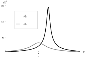
Figure 3: The ratios $\rho_{23}^{u,d}$ of the two magnitudes $|\vec{\xi}_{2}^{u,d}|=\sqrt{m_{2j}^{2}}$ and $|\vec{\xi}_{3}^{u,d}|=\sqrt{m_{3j}^{2}}$ for the up (gray curve) and down quark (black curve) triangular matrices as a function of the angle $\beta$.

Furthermore, we observe that textures with two-zeroes have the tendency to be aligned, so up and down quark mass matrices show the same hierarchy in their ‘vector like’ pattern. For small ranges around $\beta\sim\frac{\pi}{4}$ the two vectors have comparable magnitudes. This latter case could fit the first set of textures obtained in our D-brane scenario, if for example we arrange the Higgs vevs so that $\kappa_{d}\gg 1$ and $\kappa_{u}\ll 1$. We also observe that using the free parameter $\beta$ we can obtain zero textures for the up-quark matrix by demanding that some of the off-diagonal $m_{U}$-entries are zero.

We may elaborate the remaining two cases of the down quark textures with two-zeroes and obtain structures similar to the other two mass matrices obtained in the D-brane construction of section 3. In Table 4 examples of texture-zeroes are presented for all three cases and in figure 4 the ratios similar to those of fig3 are depicted.

Case	$\beta$	$m_{U}$	$m_{D}$
$A$	$\frac{\pi}{1.952}$	$\left(\begin{array}[]{ccc}0.293&0&0\\ 65.036&158.149&0\\ 1.264&0&0.0134\end{array}\right)$	$\left(\begin{array}[]{ccc}0.005&0&0\\ 0&4.247&0\\ 0&-0.165&0.125\end{array}\right)$
	$\frac{\pi}{1.928}$	$\left(\begin{array}[]{ccc}0.293&0&0\\ 65.048&158.119&0\\ 0&-3.073&0.0133\end{array}\right)$	$\left(\begin{array}[]{ccc}0.005&0&0\\ 0&4.243&0\\ 0&-0.248&0.125\end{array}\right)$
	$\frac{\pi}{53.86}$	$\left(\begin{array}[]{ccc}0.293&0&0\\ 0&3.073&0\\ 65.048&158.118&0.684\end{array}\right)$	$\left(\begin{array}[]{ccc}0.005&0&0\\ 0&0.277&0\\ 0&3.786&1.915\end{array}\right)$
$B$	$\frac{\pi}{1.973}$	$\left(\begin{array}[]{lll}7.226&0&0\\ 0&0.249&0\\ -168.576&27.791&0.342\end{array}\right)$	$\left(\begin{array}[]{lll}0.120&0&0\\ -0.003&0.005&0\\ 0&0&4.25\end{array}\right)$
	$\frac{\pi}{200}$	$\left(\begin{array}[]{lll}0.253&0&0\\ -1.174&7.130&0\\ 0&-170.851&0.342\end{array}\right)$	$\left(\begin{array}[]{lll}0.005&0&0\\ 0.0420&0.112&0\\ 0&0&4.25\end{array}\right)$
$C$	$\frac{\pi}{2}$	$\left(\begin{array}[]{lll}170.851&0&0\\ -7.129&1.170&0\\ 0&0.271&0.003\end{array}\right)$	$\left(\begin{array}[]{lll}4.25&0&0\\ 0&0.12&0\\ 0.003&0&0.005\end{array}\right)$

Table 4: Examples of the three cases $A,B,C$ of the two-zeroes down quark (Cholesky) mass textures. The specific values of the free parameter $\beta$ result also to up quark textures with one zero. $\beta$-angle values around $\frac{\pi}{2}$ inverse the hierarchy. In particular, $|\xi_{2}^{u}|>|\xi_{3}^{u}|>|\xi_{1}^{u}|$ in $A$, $|\xi_{3}^{u}|>|\xi_{1}^{u}|>|\xi_{2}^{u}|$ in $B$ and $|\xi_{1}^{u}|>|\xi_{2}^{u}|>|\xi_{3}^{u}|$ in $C$.

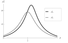
Figure 4: The ratios $\rho_{12}^{u,d}$ and $\rho_{13}^{u,d}$ as in figure 3.

6.2 One-zero Textures

Next, we investigate the consistency conditions in a simple example with one-zero texture. We have seen in the previous section that one-zero triangular mass matrices are possible provided that certain relations are imposed between the elements of the diagonalizing and the mass matrices. For example, imposing (182), we obtain $\vec{\xi}_{2}\cdot\hat{e}_{1}=0$ i.e., a one-zero texture. We have further stressed that to avoid any other zero off-diagonal entry we must demand $u_{1j}\neq 0$ and $u_{2j}\neq 0$. To obtain the simplest admissible one-zero texture, let us assume however, that some of the remaining entries of the orthogonal matrix is zero, i.e., $u_{3j}=0$ for some $j$. From (182) we have $m_{j}^{2}=A_{kk}$ which implies the relation

$$u_{kl}^{2} = \frac{m_{j}^{2}-m_{i}^{2}}{m_{l}^{2}-m_{j}^{2}}\,u_{ki}^{2}$$ (210)

with $i\neq j\neq l\neq i$ and $k=1,2$. Since $u_{kl}^{2},u_{ki}^{2}$ are always positive, and the mass hierarchies are $m_{3}>m_{2}>m_{1}$, the relation is valid only for $i=1,j=2,l=3$. Thus we get

$$u_{13} = \tan\phi_{0}\,u_{11}$$ (211)

$$u_{23} = \tan\phi_{0}\,u_{21}$$ (212)

and

$$\tan\phi_{0}=\sqrt{\frac{m_{2}^{2}-m_{1}^{2}}{m_{3}^{2}-m_{2}^{2}}}$$ (213)

Working out the details, we find

$$V_{d} = \left(\begin{array}[]{ccc}\cos\theta\cos\phi_{0}&-\sin\theta&-\cos\theta\sin\phi_{0}\\ \cos\phi_{0}\sin\theta&\cos\theta&-\sin\theta\sin\phi_{0}\\ \sin\phi_{0}&0&\cos\phi_{0}\end{array}\right)$$ (217)

where $\theta$ an arbitrary angle. In the notation of section 5, this can be considered as a combined rotation of two orthogonal matrices

$$U(\theta)=\exp[\vec{v}_{\theta}\cdot\vec{s}] U(\phi_{0})=\exp[\vec{v}_{\phi_{0}}\cdot\vec{s}]$$ , (218)

with ‘vectors’

$$\vec{v}_{\theta}=\left(0,-\sin\frac{\theta}{2},0\right) \vec{v}_{\phi_{0}}=\left(0,0,-\sin\frac{\phi_{0}}{2}\right)$$

In the same notation, the corresponding ‘vector’ of the combined matrix (217) is computed adapting appropriately the formula (119) for the convolution $U(\theta)U(\phi_{0})$

$$\vec{v}_{d}(\theta,\phi_{0}) = \left(-\sin\frac{\theta}{2}\sin\frac{\phi_{0}}{2},-\cos\frac{\theta}{2}\sin\frac{\phi_{0}}{2},-\sin\frac{\theta}{2}\cos\frac{\phi_{0}}{2}\right)$$ (219)

For arbitrary $(\theta,\phi)$ the geometrical locus of the tip of this vector is plotted in figure 5.

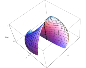
Figure 5: Part of the two-dimensional surface spanned by the vector $\vec{v}_{3}(\theta,\phi)$. Down quark masses fix one parameter $\phi=\phi_{0}$ and the two dimensional surface reduces to the thick curve.

Given the down quark mass hierarchies and the formula (213) the angle $\phi$ takes only a specific value $\phi_{0}$ and the ‘motion’ of the vector tip is constrained along the curve $\phi=\phi_{0}$. We conclude that, unless the free parameter $\theta$ is close to $\theta\sim 2n\pi,n=0,1,2...$, the $\vec{v}_{d}$ indicates a rotation mainly around the third axis. The corresponding ‘vector’ of the up-quark diagonalizing matrix can be computed using again the very same formula (119) where now the combining vectors are the CKM and $\vec{v}_{d}$. The third components of both vectors $v_{d},v_{u}$ for $\phi=\phi_{0}$ are plotted in figure 6.

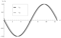
Figure 6: The third components of the vectors of the up and down diagonalizing matrices in the representation (121) as a function of the free parameter in the one-zero texture example of the text.

The down quark mass matrix is

$$m_{D} = \left(\begin{array}[]{ccc}m_{2}&0&0\\ 0&m_{2}&0\\ -\frac{\cos\theta\sqrt{(m_{2}^{2}-m_{1}^{2})(m_{3}^{2}-m_{2}^{2})}}{m_{2}}&-\frac{\sin\theta\sqrt{(m_{2}^{2}-m_{1}^{2})(m_{3}^{2}-m_{2}^{2})}}{m_{2}}&\frac{m_{1}m_{3}}{m_{2}}\end{array}\right)$$ (223)

For the limiting values $\theta=0,\frac{\pi}{2}$ of the only free parameter $\theta$ we recover specific patterns of the texture with two zeroes of the previous analysis. We find the following hierarchy of the vector magnitudes,

$$|\vec{\xi}_{1}^{d}|=|\vec{\xi}_{2}^{d}|=m_{2}\ll|\vec{\xi}_{3}^{d}|=\sqrt{m_{3}^{2}-m_{2}^{2}+m_{1}^{2}}$$

while as expected they satisfy the relation $|{\vec{\xi}_{1}^{d}}|^{2}+|{\vec{\xi}_{2}^{d}}|^{2}+|{\vec{\xi}_{3}^{d}}|^{2}=m_{1}^{2}+m_{2}^{2}+m_{3}^{2}$. It is straightforward to use the developed formalism and derive the corresponding analytic expressions for the up-quarks. It can be checked that consistency with the experimental data requires also the same hierarchy between the third $|\vec{\xi}_{3}^{u}|$ and the other two $|\vec{\xi}_{1,2}^{u}|$ vectors for the up-quark mass matrix, however, for ranges of $\theta$ the ratio $\frac{|\vec{\xi}^{u}_{1}|}{|\vec{\xi}^{u}_{2}|}$ could be reversed. To demonstrate this, we plot the ratios $\frac{|\vec{\xi}^{u}_{1}|}{|\vec{\xi}^{u}_{3}|},\frac{|\vec{\xi}^{u}_{2}|}{|\vec{\xi}^{u}_{3}|}$ in figure 7 as a function of the free parameter $\theta$.

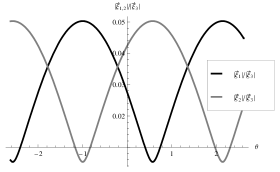
Figure 7: The ratios $\frac{|\vec{\xi}_{1}|}{|\vec{\xi}_{3}|}$ and $\frac{|\vec{\xi}_{2}|}{|\vec{\xi}_{3}|}$ of the up-quark “line-vector” magnitudes in the one zero texture as function of the free parameter $\theta$.

In this example, we have dealt with an one-zero $m_{D}$- texture while we restricted further the investigation imposing also the condition $u_{32}=0$ on the corresponding diagonalizing matrix. It is worth seeing also whether we can minimize the number of parameters in the up-quark mass matrix. Since we have one free parameter, we might choose an appropriate value to generate a texture zero case for the up quarks too. Thus, for example, choosing $\theta\sim-\frac{\pi}{3.135}$ we get

$$m_{U} \approx \left(\begin{array}[]{lll}8.58841&0&0\\ 0&0.909606&0\\ -169.892&17.458&0.0827412\end{array}\right)$$ (227)

$$m_{D} \approx \left(\begin{array}[]{lll}0.12&0&0\\ 0&0.12&0\\ -2.30052&3.56712&0.177083\end{array}\right)$$ (231)

$$V_{CKM} = \left(\begin{array}[]{lll}0.974184&0.225585&0.00877843\\ -0.225755&0.973331&0.0407647\\ 0.000651602&-0.0416941&0.99913\end{array}\right)$$ (235)

i.e., a one-zero texture, with zero entry $m_{21}=0$. The up-quark structure resembles that of case (16) obtained in the context of D-brane scenarios. The compatibility of the down quark mass matrix would be possible in the presence of a second Higgs doublet $H_{d}^{\prime}$ with appropriate vev so that $\kappa_{d}>1$.

$\theta$	$m_{U}$	$m_{D}$
$-\frac{\pi}{3.135}$	$\left(\begin{array}[]{lll}8.59&0&0\\ 0&0.91&0\\ -169.9&17.46&0.08\end{array}\right)$	$\left(\begin{array}[]{lll}0.12&0&0\\ 0&0.12&0\\ -2.30&3.57&0.177\end{array}\right)$
	$\left(\begin{array}[]{lll}1.04&0.62&-8.50\\ 0.62&0.65&0.12\\ -8.50&0.12&170.58\end{array}\right)$	$\left(\begin{array}[]{lll}0.09&0.05&-0.07\\ 0.05&0.041&0.10\\ -0.07&0.10&4.25\end{array}\right)$

Table 5: Case of one-zero up- and down quark (Cholesky) mass textures $m_{21}^{u}=m_{21}^{d}=0$ and “reversed hierarchy” for the up-quarks $|\vec{\xi}_{1,3}^{u}|>|\vec{\xi}_{2}^{u}|$. Their corresponding symmetric forms are shown in the second line.

$\theta$	$m_{U}$	$m_{D}$
$-\frac{\pi}{13.8}$	$\left(\begin{array}[]{lll}6.20&0&0\\ 5.88&1.26&0\\ -170.79&0&0.08\end{array}\right)$	$\left(\begin{array}[]{lll}0.12&0&0\\ 0&0.12&0\\ -4.14&0.96&0.18\end{array}\right)$
	$\left(\begin{array}[]{lll}0.23&0.21&-6.19\\ 0.21&1.461&-5.83\\ -6.19&-5.83&170.58\end{array}\right)$	$\left(\begin{array}[]{lll}0.014&0.025&-0.117\\ 0.025&0.114&0.028\\ -0.117&0.028&4.247\end{array}\right)$

Table 6: Case of one-zero up- and down quark (Cholesky) mass textures $m_{32}^{u}=m_{21}^{d}=0$ and “ hierarchy” for the up-quarks $|\vec{\xi}_{1}^{u}|\sim|\vec{\xi}_{2}^{u}|\ll|\vec{\xi}_{3}^{u}|$. Their corresponding symmetric forms are shown in the second line.

$\frac{\pi}{5.384}$	$\left(\begin{array}[]{lll}0.91&0&0\\ -0.87&8.54&0\\ 0&-170.79&0.08\end{array}\right)$	$\left(\begin{array}[]{lll}0.12&0&0\\ 0&0.12&0\\ -3.54&-2.34&0.18\end{array}\right)$
	$\left(\begin{array}[]{lll}0.66&-0.63&-0.03\\ -0.63&1.02&-8.50\\ -0.03&-8.50&170.58\end{array}\right)$	$\left(\begin{array}[]{lll}0.04&-0.05&-0.10\\ -0.05&0.09&-0.075\\ -0.10&-0.07&4.25\end{array}\right)$

Table 7: Cases of one-zero mass textures with $m_{21}^{d}=0$ and $m_{31}^{u}=0$ and their corresponding symmetric forms.

All the three possible cases $m_{21}=0,m_{31}=0,m_{32}=0$ can be obtained choosing appropriate values of the free parameter $\theta$ and are presented respectively in tables 5,6 and 7. These matrices are ostensibly different, however they encode the same physical properties, i.e., they result to the same eigenvalues of $m_{U,D}m_{U,D}^{T}$ and predict the CKM mixing matrix.

7 Conclusions

In this work we have examined the fermion masses in a wide class of effective low energy models emerging from intersecting D-brane configurations where the Yukawa superpotential terms are subject to additional restrictions from surplus $U(1)$ symmetries and anomaly cancelation conditions. We have shown that masses for all fermion generations are obtained only when additional Higgs doublets, or higher order corrections or substantially suppressed non-perturbative effects are taken into account. We have worked out in detail the spectrum of a representative model with Standard Model gauge symmetry augmented by abelian factors and we have observed that the fermion mass matrices exhibit a characteristic pattern which appears in a wide class of models obtained in the context of D-brane scenarios. We investigated specific cases of these novel patterns derived for the quark mass matrices and analyzed in detail the conditions imposed by phenomenological constraints on the various mass generating mechanisms in these constructions. Furthermore, motivated by the above considerations, in this work we developed a novel formalism which leads to a unified treatment of all viable symmetric and non-symmetric fermion mass textures. More precisely, we showed that the Cholesky decomposition of the mass matrices captures the features in a unique way of a whole equivalent class of mass matrices which are related to the former by an orthogonal matrix. The entries of the corresponding triangular (Cholesky) mass matrix were determined analytically in terms of the eigenmasses and the diagonalizing matrix while they were used to explore equivalent classes of symmetric and non-symmetric quark mass matrices which reconcile the hierarchical quark mass pattern and the Cabbibo-Kobayashi-Maskawa mixing matrix. We have further shown that the triangular form of the quark mass matrices admit texture-zero forms, minimizing thus the number of arbitrary parameters. A detailed analysis is presented for the D-brane derived quark mass patterns and conditions on the various mass generating sources are specified to reconcile the known mass hierarchies and mixing data. Finally, a comparison with the symmetric texture-zero quark mass matrices existing in the literature is also worked out.

Acknowledgements. This work is partially supported by the European Research and Training Network MRTPN-CT-2006 035863-1 (UniverseNet).

8 Appendix

8.1 The CKM matrix

In this appendix we will provide a few more details on the derivation of the CKM matrix in the basis $s_{1},s_{2},s_{3}$ discussed in section 4.

For the sake of clarity of the our calculations, first we review in brief the conventions used with respect to the diagonalizing matrices of the up and down quarks. We find also convenient to adopt here the Wolfenstein parametrization of the CKM matrix.

Let the weak and mass eigenstates of the up-quarks be related by the orthogonal matrices $V_{u}^{L,R}$

$$u_{L}^{0} = V_{u}^{L}\,u_{L}$$

$$u_{R}^{0} = V_{u}^{R}\,u_{R}$$

The relevant Yukawa terms are written

$$\bar{u}_{L}^{0}m_{U}u_{R}^{0} = \bar{u}_{L}V_{u}^{L\dagger}m_{U}V_{u}^{R}u_{R}$$ (236)

$$= \bar{u}_{L}m_{U}^{diag.}u_{R}$$

and similarly for the down quarks. Thus, the diagonal mass matrices are given in terms of the orthogonal transformations $V_{u}^{L,R}$ and $V_{d}^{L,R}$ respectively as follows

$$m_{U}^{diag.} = V_{u}^{L\dagger}m_{U}V_{u}^{R}$$ (237)

$$m_{D}^{diag.} = V_{d}^{L\dagger}m_{D}V_{d}^{R}$$ (238)

Since ${\left(V_{u}^{L\dagger}m_{U}V_{u}^{R}\right)}^{\dagger}=V_{u}^{R\dagger}m_{U}^{{\dagger}}V_{u}^{L}$ we get

$$\left(m_{U}^{diag.}\right)^{2} = \left(V_{u}^{L\dagger}m_{U}V_{u}^{R}\right)\left(V_{u}^{R\dagger}m_{U}^{\dagger}{V_{u}^{L}}\right)$$ (239)

$$= V_{u}^{L\dagger}m_{U}\,m_{U}^{\dagger}{V_{u}^{L}}$$

and similarly for the down quark matrix$m_{D}$ . Thus

$$m_{U}\,m_{U}^{\dagger} = {V_{u}^{L}}\,\left(m_{U}^{diag.}\right)^{2}V_{u}^{L\dagger}$$

$$m_{D}\,m_{D}^{\dagger} = {V_{d}^{L}}\,\left(m_{D}^{diag.}\right)^{2}V_{d}^{L\dagger}$$

The current is written

$$J_{W}^{\mu} = \bar{u}_{L}^{0}\gamma^{\mu}d_{L}^{0}\;=\;\bar{u}_{L}V_{u}^{L\dagger}\gamma^{\mu}V_{d}^{L}\,d_{L}$$ (240)

$$\equiv \bar{u}_{L}\gamma^{\mu}V_{CKM}d_{L}$$

where the CKM matrix is defined

$$V_{CKM} = V_{u}^{L\dagger}\,V_{d}^{L}$$ (241)

Using the Wolfenstein parametrization, the CKM matrix is expressed as follows

$$V_{KM} = \left(\begin{array}[]{ccc}1-\frac{\lambda^{2}}{2}&\lambda&A\lambda^{3}(\rho-\imath\,\eta)\\ -\lambda&1-\frac{\lambda^{2}}{2}&A\lambda^{2}\\ A\lambda^{3}(1-\rho-\imath\,\eta)&-A\lambda^{2}&1\end{array}\right)$$ (245)

with $\lambda\sim 0.2257$ and $A,\rho,\eta$ are order one parameters.

The numerical values of the CKM entries are given by [26]

$$V_{CKM}=\begin{bmatrix}0.97419&0.2257&0.00359\\ -0.2256&0.97334&0.0415\\ 0.00874&-0.0407&0.999133\end{bmatrix}~{}.$$ (246)

Taking the logarithm of $V_{CKM}$ we get

$$\ln V_{CKM}=\begin{bmatrix}0&0.2277&-0.012\\ -0.2277&0&0.0417\\ 0.0041&-0.0415&0\end{bmatrix}~{}.$$ (247)

$\ln V_{CKM}$ is not exactly antisymmetric reflecting the fact that $V_{CKM}$ is not exactly orthogonal because of experimental uncertainties. We may choose

$$\left(\ln V^{\prime}_{CKM}\right)=\begin{bmatrix}0&0.2277&-0.012\\ -0.2277&0&0.0416\\ 0.012&-0.0416&0\end{bmatrix}$$ (248)

giving

$$V^{\prime}_{CKM}=\begin{bmatrix}0.9741&0.2259&-0.0072\\ -0.2254&0.9733&0.0426\\ 0.0166&-0.0399&0.9991\end{bmatrix}$$ (249)

or

$$\left(\ln V^{\prime}_{CKM}\right)=\begin{bmatrix}0&0.2277&-0.0041\\ -0.2277&0&0.0416\\ 0.0041&-0.0416&0\end{bmatrix}$$ (250)

giving

$$V^{\prime}_{CKM}=\begin{bmatrix}0.9742&0.2258&0.0007\\ -0.2256&0.9733&0.0417\\ 0.0088&-0.0408&0.9991\end{bmatrix}$$ (251)

a clearly better choice, suitable for our numerical investigations. This way the CKM matrix can be written as

$$\ln V_{CKM}=0.0416s_{1}-0.0041s_{2}+0.2277s_{3}~{}$$ (252)

or

$$\ln V_{CKM}=\phi_{c}\widehat{n}\overrightarrow{s}$$ (253)

where $\phi_{c}=0.231505$ and

$$\widehat{n}=\begin{bmatrix}0.179694\\ 0.0177102\\ 0.983564\end{bmatrix}~{}\cdot$$ (254)

The angle $\phi_{c}$ and the unit vector $\hat{n}$ encompass all the information of the CKM matrix. From a ‘geometric’ perspective, the CKM can be viewed as rotations around three axes defined along the components of $\hat{n}$. From (254) we can observe that the rotation is predominantly around the third axis, reflect the fact that the large mixing is between the first two generations.

8.2 Cholesky form of the symmetric zero-textures

The five symmetric texture-zero mass matrices for the up and down quarks or ref. [8] admit the following Cholesky form

1. $$m_{U}=\begin{bmatrix}\sqrt{2}\varepsilon^{6}&0&0\\ \varepsilon^{4}&\sqrt{2}\varepsilon^{6}&0\\ 0&0&1\end{bmatrix},m_{D}=\begin{bmatrix}2\varepsilon^{4}&0&0\\ 2\varepsilon^{3}&4\varepsilon^{3}\sqrt{1+\frac{1}{4}\varepsilon^{2}}&0\\ 4\varepsilon^{3}&\frac{1}{\sqrt{1+\frac{1}{4}\varepsilon^{2}}}&\frac{\varepsilon}{2\sqrt{1+\frac{1}{4}\varepsilon^{2}}}\end{bmatrix}$$ (255)

2. $$m_{U}=\begin{bmatrix}\varepsilon^{6}&0&0\\ 0&\varepsilon^{2}\sqrt{1+\varepsilon^{8}}&0\\ \varepsilon^{2}&\frac{1}{\sqrt{1+\varepsilon^{8}}}&\frac{\varepsilon^{4}}{\sqrt{1+\varepsilon^{8}}}\end{bmatrix},m_{D}=\begin{bmatrix}2\varepsilon^{4}&0&0\\ 2\varepsilon^{3}&2\varepsilon^{3}\sqrt{1+\varepsilon^{2}}&0\\ 2\varepsilon^{3}&\frac{1}{\sqrt{1+\varepsilon^{2}}}&\frac{\varepsilon}{\sqrt{1+\varepsilon^{2}}}\end{bmatrix}$$ (256)

3. $$m_{U}=\begin{bmatrix}\sqrt{2}\varepsilon^{4}&0&0\\ 0&\varepsilon^{4}&0\\ 1&0&\sqrt{2}\varepsilon^{4}\end{bmatrix}m_{D}=\begin{bmatrix}2\varepsilon^{4}&0&0\\ 2\varepsilon^{3}&4\varepsilon^{3}\sqrt{1+\frac{1}{4}\varepsilon^{2}}&0\\ 4\varepsilon^{3}&\frac{1}{\sqrt{1+\frac{1}{4}\varepsilon^{2}}}&\frac{1}{2}\frac{\varepsilon}{\sqrt{1+\frac{1}{4}\varepsilon^{2}}}\end{bmatrix}$$ (257)

4. $$m_{U}=\begin{bmatrix}\sqrt{2}\varepsilon^{6}&0&0\\ \sqrt{3}\varepsilon^{4}&\varepsilon^{2}\sqrt{1+2\varepsilon^{8}}&0\\ \varepsilon^{2}&\frac{1}{\sqrt{1+2\varepsilon^{8}}}&\frac{\sqrt{2}\varepsilon^{4}}{\sqrt{1+2\varepsilon^{8}}}\end{bmatrix},m_{D}=\begin{bmatrix}2\varepsilon^{4}&0&0\\ 2\varepsilon^{3}&2\varepsilon^{4}&0\\ 0&0&1\end{bmatrix}$$ (258)

5. $$m_{U}=\begin{bmatrix}\varepsilon^{4}&0&0\\ \frac{1}{\sqrt{2}}\varepsilon^{2}&\sqrt{2}\varepsilon^{4}&0\\ 1&\frac{1}{\sqrt{2}}\varepsilon^{2}&\varepsilon^{4}\end{bmatrix},m_{D}=\begin{bmatrix}2\varepsilon^{4}&0&0\\ 2\varepsilon^{3}&2\varepsilon^{4}&0\\ 0&0&1\end{bmatrix}$$ (259)

8.3 Textures with two-zeroes

In this section we will derive the complete list of triangular texture with two-zeroes with their corresponding orthogonal diagonalizing matrices. As we have seen in the text, the orthogonal matrix is given by

$$U_{a}=\exp\left[a\widehat{n}\cdot\overrightarrow{s}\right]=1+\sin a~{}\widehat{n}\cdot\overrightarrow{s}+\left(1-\cos a\right)\left(\widehat{n}\cdot\overrightarrow{s}\right)^{2}\cdot$$ (260)

where $\hat{n}$ is a unit vector and $\vec{s}=(s_{1},s_{2},s_{3})$ with $s_{i}$ the matrices given in (105). The matrices (105) satisfy the algebra

$$\left[s_{i},~{}s_{j}\right]=\varepsilon_{ijk}s_{k}$$ (261)

and their eigenvalues are $\pm i$ and $0$. For computational purposes we also notice that

$$\left(\widehat{n}\cdot\overrightarrow{s}\right)^{3}=-\widehat{n}\cdot\overrightarrow{s}$$ (262)

and the ‘commutation’ relation

$$\left[\overrightarrow{a}\cdot\overrightarrow{s},~{}~{}\overrightarrow{b}\cdot\overrightarrow{s}\right]=\left(\overrightarrow{a}\times\overrightarrow{b}\right)\cdot\overrightarrow{s}$$ (263)

We have redefined also the vector $\widehat{n}$

$$\widehat{n}\rightarrow\sin\frac{a}{2}\widehat{n}\equiv\overrightarrow{n}~{}\cdot$$ (264)

and the new vector $\overrightarrow{n}$ assumes the components $(a_{1},a_{2},a_{3})$ where now

$$\overrightarrow{n}^{2}=a_{1}^{2}+a_{2}^{2}+a_{3}^{2}=\sin^{2}\frac{\alpha}{2}\cdot$$ (265)

The orthogonal matrix $U_{\alpha}$ is finally written

$$U_{\alpha}=1+2\cos\frac{\alpha}{2}\overrightarrow{n}\cdot\overrightarrow{s}+2\left(\overrightarrow{n}\cdot\overrightarrow{s}\right)^{2}$$ (266)

while in expanded form we get

$$U_{\alpha}=\begin{bmatrix}\cos\alpha+2a_{1}^{2}&2\left(a_{3}\cos\frac{\alpha}{2}-a_{1}a_{2}\right)&2\left(a_{2}\cos\frac{\alpha}{2}+a_{1}a_{3}\right)\\ -2\left(a_{3}\cos\frac{\alpha}{2}+a_{1}a_{2}\right)&\cos\alpha+2a_{2}^{2}&2\left(a_{1}\cos\frac{\alpha}{2}-a_{2}a_{3}\right)\\ -2\left(a_{2}\cos\frac{\alpha}{2}-a_{1}a_{3}\right)&-2\left(a_{1}\cos\frac{\alpha}{2}+a_{2}a_{3}\right)&\cos\alpha+2a_{3}^{2}\end{bmatrix}~{}.$$ (267)

In addition to the cases discussed in the text, zero elements are generated whenever we have

$$a_{1} = \pm\cos\frac{\alpha}{2}$$ (268)

$$a_{2} = \pm a_{3}=\sqrt{-\frac{1}{2}\cos\alpha}$$ (269)

plus permutations. It is obvious that because of the square root we need $\cos\alpha<0$. The matrix $U_{\alpha}$ acquires four zero elements and one element equal to $\pm 1~{}$. From the remaining four elements only two are independent and equal

$$\rho_{1} = 1+2\cos\alpha$$ (270)

$$\rho_{2} = 2\sqrt{2}\cos\frac{\alpha}{2}\sqrt{-\cos\alpha}~{}\cdot$$ (271)

Note that since $\cos\alpha<0$, the range of $\rho_{1}=[-1,1]$ while

$$\rho_{1}^{2}+\rho_{2}^{2}=1$$ (272)

i.e. the $2\times 2$ submatrix is orthogonal, thus we may put $\rho_{1}=\cos\theta,\rho_{2}=\sin\theta$.

Below we give a list all the cases that generate zeroes together with the corresponding $U_{\alpha}$ and $MM^{T}$ matrices. To simplify the forthcoming formulae we define the matrix

$${\cal M} = \left(\begin{array}[]{ccc}m_{1}^{2}&0&0\\ 0&m_{2}^{2}&0\\ 0&0&m_{3}^{2}\end{array}\right)$$ (276)

Also, the sign symbols appearing bellow correspond to the signs of $a_{1}$ $a_{2}$ and $a_{3}$ respectively. This way we get ($\cos\theta\rightarrow c,\sin\theta\rightarrow s$):

• $a_{1}~{}a_{2}~{}a_{3}$

  $$\begin{bmatrix}+&+&+\end{bmatrix},\;~{}U=\begin{bmatrix}c&0&s\\ -s&0&c\\ 0&-1&0\end{bmatrix}$$

  $$U{\cal M}U^{T}=\begin{bmatrix}c^{2}m_{1}^{2}+s^{2}m_{3}^{2}&cs\left(m_{3}^{2}-m_{1}^{2}\right)&0\\ cs\left(m_{3}^{2}-m_{1}^{2}\right)&c^{2}m_{3}^{2}+s^{2}m_{1}^{2}&0\\ 0&0&m_{2}^{2}\end{bmatrix}$$

  $$\begin{bmatrix}+&+&-\end{bmatrix}\,,~{}U=\begin{bmatrix}c&-s&0\\ 0&0&1\\ -s&-c&0\end{bmatrix}$$

  $$U{\cal M}U^{T}=\begin{bmatrix}c^{2}m_{1}^{2}+s^{2}m_{2}^{2}&0&cs\left(m_{2}^{2}-m_{1}^{2}\right)\\ 0&m_{3}^{2}&0\\ cs\left(m_{2}^{2}-m_{1}^{2}\right)&0&c^{2}m_{2}^{2}+s^{2}m_{1}^{2}\end{bmatrix}$$

  $$\begin{bmatrix}+&-&+\end{bmatrix},\,~{}U=\begin{bmatrix}c&s&0\\ 0&0&1\\ s&-c&0\end{bmatrix}$$

  $$U{\cal M}U^{T}=\begin{bmatrix}c^{2}m_{1}^{2}+s^{2}m_{2}^{2}&0&s\,c\left(m_{1}^{2}-m_{2}^{2}\right)\\ 0&m_{3}^{2}&0\\ c\,s_{2}\left(m_{1}^{2}-m_{2}^{2}\right)&0&c^{2}m_{2}^{2}+s^{2}m_{1}^{2}\end{bmatrix}$$

  $$\begin{bmatrix}+&-&-\end{bmatrix}\,,~{}U=\begin{bmatrix}c&0&-s\\ s&0&c\\ 0&-1&0\end{bmatrix}$$

  $$U{\cal M}U^{T}=\begin{bmatrix}c^{2}m_{1}^{2}+s^{2}m_{3}^{2}&c\,s\left(m_{1}^{2}-m_{3}^{2}\right)&0\\ c\,s\left(m_{1}^{2}-m_{3}^{2}\right)&c^{2}m_{3}^{2}+s^{2}m_{1}^{2}&0\\ 0&0&m_{2}^{2}\end{bmatrix}$$

  $$\begin{bmatrix}-&+&+\end{bmatrix}\,,~{}U=\begin{bmatrix}c&s&0\\ 0&0&-1\\ -s&c&0\end{bmatrix}$$

  $$U{\cal M}U^{T}=\begin{bmatrix}c^{2}m_{1}^{2}+s^{2}m_{2}^{2}&0&c\,s\left(m_{2}^{2}-m_{1}^{2}\right)\\ 0&m_{3}^{2}&0\\ c\,s\left(m_{2}^{2}-m_{1}^{2}\right)&0&c^{2}m_{2}^{2}+s^{2}m_{1}^{2}\end{bmatrix}$$

  $$\begin{bmatrix}-&+&-\end{bmatrix}\,,~{}U=\begin{bmatrix}c&0&s\\ s&0&-c\\ 0&1&0\end{bmatrix}$$

  $$~{}U{\cal M}U^{T}=\begin{bmatrix}c^{2}m_{1}^{2}+s^{2}m_{3}^{2}&c\,s\left(m_{1}^{2}-m_{3}^{2}\right)&0\\ c\,s\left(m_{1}^{2}-m_{3}^{2}\right)&c^{2}m_{3}^{2}+s^{2}m_{1}^{2}&0\\ 0&0&m_{2}^{2}\end{bmatrix}$$

  $$\begin{bmatrix}-&-&+\end{bmatrix}\,,~{}U=\begin{bmatrix}c&0&-s\\ -s&0&-c\\ 0&1&0\end{bmatrix}$$

  $$~{}U{\cal M}~{}U^{T}=\begin{bmatrix}c^{2}m_{1}^{2}+s^{2}m_{3}^{2}&cs\left(m_{3}^{2}-m_{1}^{2}\right)&0\\ cs\left(m_{3}^{2}-m_{1}^{2}\right)&c^{2}m_{3}^{2}+s^{2}m_{1}^{2}&0\\ 0&0&m_{2}^{2}\end{bmatrix}$$

  $$\begin{bmatrix}-&-&-\end{bmatrix}\,,~{}U=\begin{bmatrix}c&-s&0\\ 0&0&-1\\ s&c&0\end{bmatrix}$$

  $$U{\cal M}U^{T}=\begin{bmatrix}c^{2}m_{1}^{2}+s^{2}m_{2}^{2}&0&cs\left(m_{1}^{2}-m_{2}^{2}\right)\\ 0&m_{3}^{2}&0\\ cs\left(m_{1}^{2}-m_{2}^{2}\right)&0&c^{2}m_{2}^{2}+s^{2}m_{1}^{2}\end{bmatrix}$$

• $a_{2}~{}a_{1}~{}a_{3}$

  $$\begin{bmatrix}+&+&+\end{bmatrix}\,,~{}U=\begin{bmatrix}0&0&1\\ -s&c&0\\ -c&-s&0\end{bmatrix}$$

  $$U{\cal M}U^{T}=\begin{bmatrix}m_{3}^{2}&0&0\\ 0&c^{2}m_{2}^{2}+s^{2}m_{1}^{2}&cs\left(m_{1}^{2}-m_{2}^{2}\right)\\ 0&cs\left(m_{1}^{2}-m_{2}^{2}\right)&c^{2}m_{1}^{2}+s^{2}m_{2}^{2}\end{bmatrix}$$

  $$\begin{bmatrix}+&+&-\end{bmatrix}\,,~{}U=\begin{bmatrix}0&-s&c\\ 0&c&s\\ -1&0&0\end{bmatrix}$$

  $$U{\cal M}U^{T}=\begin{bmatrix}c^{2}m_{3}^{2}+s^{2}m_{2}^{2}&cs\left(m_{3}^{2}-m_{2}^{2}\right)&0\\ cs\left(m_{3}^{2}-m_{2}^{2}\right)&c^{2}m_{2}^{2}+s^{2}m_{3}^{2}&0\\ 0&0&m_{1}^{2}\end{bmatrix}$$

  $$\begin{bmatrix}+&-&+\end{bmatrix}\,,~{}U=\begin{bmatrix}0&s&c\\ 0&c&-s\\ -1&0&0\end{bmatrix}$$

  $$U{\cal M}U^{T}=\begin{bmatrix}c^{2}m_{3}^{2}+s^{2}m_{2}^{2}&cs\left(m_{2}^{2}-m_{3}^{2}\right)&0\\ cs\left(m_{2}^{2}-m_{3}^{2}\right)&c^{2}m_{2}^{2}+s^{2}m_{3}^{2}&0\\ 0&0&m_{1}^{2}\end{bmatrix}$$

  $$\begin{bmatrix}+&-&-\end{bmatrix}\,,~{}U=\begin{bmatrix}0&0&1\\ s&c&0\\ -c&s&0\end{bmatrix}$$

  $$U{\cal M}U^{T}=\begin{bmatrix}m_{3}^{2}&0&0\\ 0&c^{2}m_{2}^{2}+s^{2}m_{1}^{2}&c\,s\left(m_{2}^{2}-m_{1}^{2}\right)\\ 0&cs\left(m_{2}^{2}-m_{1}^{2}\right)&c^{2}m_{1}^{2}+s^{2}m_{2}^{2}\end{bmatrix}$$

  $$\begin{bmatrix}-&+&+\end{bmatrix}\,,~{}U=\begin{bmatrix}0&s&-c\\ 0&c&s\\ 1&0&0\end{bmatrix}$$

  $$U{\cal M}U^{T}=\begin{bmatrix}c^{2}m_{3}^{2}+s^{2}m_{2}^{2}&cs\left(m_{2}^{2}-m_{3}^{2}\right)&0\\ cs\left(m_{2}^{2}-m_{3}^{2}\right)&c^{2}m_{2}^{2}+s^{2}m_{3}^{2}&0\\ 0&0&m_{1}^{2}\end{bmatrix}$$

  $$\begin{bmatrix}-&+&-\end{bmatrix}\,,~{}U=\begin{bmatrix}0&0&-1\\ s&c&0\\ c&-s&0\end{bmatrix}$$

  $$U{\cal M}U^{T}=\begin{bmatrix}m_{3}^{2}&0&0\\ 0&c^{2}m_{2}^{2}+s^{2}m_{1}^{2}&cs\left(m_{1}^{2}-m_{2}^{2}\right)\\ 0&cs\left(m_{1}^{2}-m_{2}^{2}\right)&c^{2}m_{1}^{2}+s^{2}m_{2}^{2}\end{bmatrix}$$

  $$\begin{bmatrix}-&-&+\end{bmatrix}\,,~{}U=\begin{bmatrix}0&0&-1\\ -s&c&0\\ c&s&0\end{bmatrix}$$

  $$U{\cal M}U^{T}=\begin{bmatrix}m_{3}^{2}&0&0\\ 0&c^{2}m_{2}^{2}+s^{2}m_{1}^{2}&cs\left(m_{2}^{2}-m_{1}^{2}\right)\\ 0&cs\left(m_{2}^{2}-m_{1}^{2}\right)&c^{2}m_{1}^{2}+s{2}m_{2}^{2}\end{bmatrix}$$

  $$\begin{bmatrix}-&-&-\end{bmatrix}\,,~{}U=\begin{bmatrix}0&-s&-c\\ 0&c&-s\\ 1&0&0\end{bmatrix}$$

  $$U{\cal M}U^{T}=\begin{bmatrix}c^{2}m_{3}^{2}+s^{2}m_{2}^{2}&cs\left(m_{3}^{2}-m_{2}^{2}\right)&0\\ cs\left(m_{3}^{2}-m_{2}^{2}\right)&c^{2}m_{2}^{2}+s^{2}m_{3}^{2}&0\\ 0&0&m_{1}^{2}\end{bmatrix}$$

• $a_{3}~{}a_{1}~{}a_{2}$

  $$\begin{bmatrix}+&+&+\end{bmatrix}\,,~{}U=\begin{bmatrix}0&c&s\\ -1&0&0\\ 0&-s&c\end{bmatrix}$$

  $$U{\cal M}U^{T}=\begin{bmatrix}c^{2}m_{2}^{2}+s^{2}m_{3}^{2}&0&cs\left(m_{3}^{2}-m_{2}^{2}\right)\\ 0&m_{1}^{2}&0\\ cs\left(m_{3}^{2}-m_{2}^{2}\right)&0&c^{2}m_{3}^{2}+s^{2}m_{2}^{2}\end{bmatrix}$$

  $$\begin{bmatrix}+&+&-\end{bmatrix}\,,~{}U=\begin{bmatrix}0&1&0\\ -c&0&s\\ s&0&c\end{bmatrix}$$

  $$U{\cal M}U^{T}=\begin{bmatrix}m_{2}^{2}&0&0\\ 0&c^{2}m_{1}^{2}+s^{2}m_{3}^{2}&cs\left(m_{3}^{2}-m_{1}^{2}\right)\\ 0&cs\left(m_{3}^{2}-m_{1}^{2}\right)&c^{2}m_{3}^{2}+s^{2}m_{1}^{2}\end{bmatrix}$$

  $$\begin{bmatrix}+&-&+\end{bmatrix}\,,~{}U=\begin{bmatrix}0&1&0\\ -c&0&-s\\ -s&0&c\end{bmatrix}$$

  $$~{}U{\cal M}U^{T}=\begin{bmatrix}m_{2}^{2}&0&0\\ 0&c^{2}m_{1}^{2}+s^{2}m_{3}^{2}&cs\left(m_{1}^{2}-m_{3}^{2}\right)\\ 0&cs\left(m_{1}^{2}-m_{3}^{2}\right)&c^{2}m_{3}^{2}+s^{2}m_{1}^{2}\end{bmatrix}$$

  $$\begin{bmatrix}+&-&-\end{bmatrix}\,,~{}U=\begin{bmatrix}0&c&-s\\ -1&0&0\\ 0&s&c\end{bmatrix}$$

  $$U{\cal M}U^{T}=\begin{bmatrix}c^{2}m_{2}^{2}+s^{2}m_{3}^{2}&0&cs\left(m_{2}^{2}-m_{3}^{2}\right)\\ 0&m_{1}^{2}&0\\ cs\left(m_{2}^{2}-m_{3}^{2}\right)&0&c^{2}m_{3}^{2}+s^{2}m_{2}^{2}\end{bmatrix}$$

  $$\begin{bmatrix}-&+&+\end{bmatrix}\,,~{}U=\begin{bmatrix}0&-1&0\\ c&0&s\\ -s&0&c\end{bmatrix}$$

  $$U{\cal M}U^{T}=\begin{bmatrix}m_{2}^{2}&0&0\\ 0&c^{2}m_{1}^{2}+s^{2}m_{3}^{2}&cs\left(m_{3}^{2}-m_{1}^{2}\right)\\ 0&cs\left(m_{3}^{2}-m_{1}^{2}\right)&c^{2}m_{3}^{2}+s^{2}m_{1}^{2}\end{bmatrix}$$

  $$\begin{bmatrix}-&+&-\end{bmatrix}\,,~{}U=\begin{bmatrix}0&-c&-s\\ 1&0&0\\ 0&-s&c\end{bmatrix}$$

  $$U{\cal M}U^{T}=\begin{bmatrix}c^{2}m_{2}^{2}+s^{2}m_{3}^{2}&0&cs\left(m_{2}^{2}-m_{3}^{2}\right)\\ 0&m_{1}^{2}&0\\ cs\left(m_{2}^{2}-m_{3}^{2}\right)&0&c^{2}m_{3}^{2}+s^{2}m_{2}^{2}\end{bmatrix}$$

  $$\begin{bmatrix}-&-&+\end{bmatrix}\,,~{}U=\begin{bmatrix}0&-c&s\\ 1&0&0\\ 0&s&c\end{bmatrix}$$

  $$U{\cal M}U^{T}=\begin{bmatrix}c^{2}m_{2}^{2}+s^{2}m_{3}^{2}&0&cs\left(m_{3}^{2}-m_{2}^{2}\right)\\ 0&m_{1}^{2}&0\\ cs\left(m_{3}^{2}-m_{2}^{2}\right)&0&c^{2}m_{3}^{2}+s^{2}m_{2}^{2}\end{bmatrix}$$

  $$\begin{bmatrix}-&-&-\end{bmatrix}\,,~{}U=\begin{bmatrix}0&-1&0\\ c&0&-s\\ s&0&c\end{bmatrix}$$

  $$U{\cal M}U^{T}=\begin{bmatrix}m_{2}^{2}&0&0\\ 0&c^{2}m_{1}^{2}+s^{2}m_{3}^{2}&cs\left(m_{1}^{2}-m_{3}^{2}\right)\\ 0&cs\left(m_{1}^{2}-m_{3}^{2}\right)&c^{2}m_{3}^{2}+s^{2}m_{1}^{2}\end{bmatrix}$$

8.4 One zero textures.

If we want the triangular matrix to have one zero element we must address the following geometrical problem. Given an orthonormal basis in the 3-d space $\overrightarrow{a}$,$\overrightarrow{b}$ and $\overrightarrow{c}=\overrightarrow{a}\times\overrightarrow{b}$   and a matrix $M$ (diagonal in our case) we must satisfy the condition

$$\overrightarrow{a}M\overrightarrow{b}=0\cdot$$ (277)

If this relation is to hold true we must have

$$M\overrightarrow{b}=\left(\overrightarrow{b}M\overrightarrow{b}\right)\overrightarrow{b}+\left(\overrightarrow{c}M\overrightarrow{b}\right)\overrightarrow{c}$$ (278)

or

$$\left[M-\overrightarrow{b}M\overrightarrow{b}\right]\overrightarrow{b}=\left(\overrightarrow{c}M\overrightarrow{b}\right)\overrightarrow{c}~{}\cdot$$ (279)

Furthermore, in order to check whether the vector $\overrightarrow{c}$ admits also zero components we must investigate the relation

$$M=\overrightarrow{b}M\overrightarrow{b}~{}\cdot$$ (280)

This relation in components gives

$$b_{2}^{2}\left(m_{1}^{2}-m_{2}^{2}\right) = b_{3}^{2}\left(m_{3}^{2}-m_{1}^{2}\right)$$ (281)

$$b_{1}^{2}\left(m_{2}^{2}-m_{1}^{2}\right) = b_{3}^{2}\left(m_{3}^{2}-m_{2}^{2}\right)$$ (282)

$$b_{1}^{2}\left(m_{3}^{2}-m_{1}^{2}\right) = b_{2}^{2}\left(m_{2}^{2}-m_{3}^{2}\right)~{}\cdot$$ (283)

Taking into account the charged fermion mass hierarchy $m_{3}>m_{2}>m_{1}$, we observe that only the second line (282) can be satisfied so that only $c_{2}$ can vanish.

Returning to (279) and taking the ratios of its components we obtain

$$\frac{c_{1}}{c_{2}}=\frac{m_{1}^{2}-\overrightarrow{b}M\overrightarrow{b}}{m_{2}^{2}-\overrightarrow{b}M\overrightarrow{b}}\frac{b_{1}}{b_{2}}\,\equiv\,a_{12}\frac{b_{1}}{b_{2}}$$ (284)

$$\frac{c_{2}}{c_{3}}=\frac{m_{2}^{2}-\overrightarrow{b}M\overrightarrow{b}}{m_{3}^{2}-\overrightarrow{b}M\overrightarrow{b}}\frac{b_{2}}{b_{3}}\,\equiv\,a_{23}\frac{b_{2}}{b_{3}}$$ (285)

$$\frac{c_{1}}{c_{3}}=\frac{m_{1}^{2}-\overrightarrow{b}M\overrightarrow{b}}{m_{3}^{2}-\overrightarrow{b}M\overrightarrow{b}}\frac{b_{1}}{b_{3}}\,\equiv\,a_{13}\frac{b_{1}}{b_{3}}~{}\cdot$$ (286)

in a self-explanatory notation. Solving for $c_{1},c_{2}$ we get

$$c_{2} = a_{23}\frac{b_{2}}{b_{3}}c_{3}$$ (287)

$$c_{1} = a_{13}\frac{b_{1}}{b_{3}}c_{3}$$ (288)

We observe that the orthogonality condition

$$b_{1}c_{1}+b_{2}c_{2}+b_{3}c_{3}=0$$ (289)

is satisfied automatically provided that

$$b_{1}^{2}+b_{2}^{2}+b_{3}^{2}=1~{}\cdot$$ (290)

Also, we find that

$$c_{1}^{2}+c_{2}^{2}+c_{3}^{2}=c_{3}^{2}\left[1+\frac{a_{23}^{2}b_{2}^{2}+a_{13}^{2}b_{1}^{2}}{b_{3}^{2}}\right]=1$$ (291)

so that the $c_{3}$ component can be expressed as a function of the mass eigenstates and the vector $\overrightarrow{b}$ as follows

$$c_{3}=\pm\frac{b_{3}}{\sqrt{a_{13}^{2}b_{1}^{2}+a_{23}^{2}b_{2}^{2}+b_{3}^{2}}}~{}\cdot$$ (292)

The remaining two components $c_{1,2}$ follow immediately, thus we finally get:

$$c_{1}=a_{13}\frac{b_{1}}{\sqrt{a_{13}^{2}b_{1}^{2}+a_{23}^{2}b_{2}^{2}+b_{3}^{2}}}$$ (293)

$$c_{2}=a_{23}\frac{b_{2}}{\sqrt{a_{13}^{2}b_{1}^{2}+a_{23}^{2}b_{2}^{2}+b_{3}^{2}}}~{}$$ (294)

$$c_{3}=\pm\frac{b_{3}}{\sqrt{a_{13}^{2}b_{1}^{2}+a_{23}^{2}b_{2}^{2}+b_{3}^{2}}}~{}\cdot$$ (295)

Depending on the sign of $c_{3}$, the vector $\overrightarrow{a}=\overrightarrow{b}\times\overrightarrow{c}$ equals

$$a_{1} = \frac{\left(1-a_{23}\right)b_{2}b_{3}}{\sqrt{a_{13}^{2}b_{1}^{2}+a_{23}^{2}b_{2}^{2}+b_{3}^{2}}}$$ (296)

$$a_{2} = \frac{\left(a_{13}-1\right)b_{1}b_{3}}{\sqrt{a_{13}^{2}b_{1}^{2}+a_{23}^{2}b_{2}^{2}+b_{3}^{2}}}$$ (297)

$$a_{3} = \frac{\left(a_{23}-a_{13}\right)b_{1}b_{2}}{\sqrt{a_{13}^{2}b_{1}^{2}+a_{23}^{2}2b_{2}^{2}+b_{3}^{2}}}$$ (298)

or

$$a_{1} = -\frac{\left(1+a_{23}\right)b_{2}b_{3}}{\sqrt{a_{13}^{2}b_{1}^{2}+a_{23}^{2}b_{2}^{2}+b_{3}^{2}}}$$ (299)

$$a_{2} = \frac{\left(1+a_{13}\right)b_{1}b_{3}}{\sqrt{a_{13}^{2}b_{1}^{2}+a_{23}^{2}b_{2}^{2}+b_{3}^{2}}}$$ (300)

$$a_{3} = \frac{\left(a_{23}-a_{13}\right)b_{1}b_{2}}{\sqrt{a_{13}^{2}b_{1}^{2}+a_{23}^{2}b_{2}^{2}+b_{3}^{2}}}\cdot$$ (301)

Thus the formulae for the $a_{i},c_{i}$ components constitute the general solution to the one-zero texture expressed by the condition (277).

Going back to the definitions of the triangular (Cholesky) matrix (100), we distinguish the following three cases with respect to the three off-diagonal entries:

$i$) To apply the above formulae for a zero $\{21\}$ element in the triangular matrix

$$\overrightarrow{\xi}_{2}\cdot\overrightarrow{e}_{1}=\frac{u_{11}u_{21}m_{1}^{2}+u_{22}u_{12}m_{2}^{2}+u_{13}u_{23}m_{3}^{2}}{\sqrt{u_{11}^{2}m_{1}^{2}+u_{12}^{2}m_{2}^{2}+u_{13}^{2}m_{3}^{2}}}$$ (302)

we make the identifications

$$\overrightarrow{a} = \left[u_{11},u_{12},u_{13}\right]$$ (303)

$$\overrightarrow{b} = \left[u_{21},u_{22},u_{23}\right]$$ (304)

$$\overrightarrow{c} = \left[u_{31},u_{32},u_{33}\right]\cdot$$ (305)

At the same time, the only allowed zero element in the orthogonal matrix is $u_{32}$, in accordance with (282).

$ii$) For a zero $\{31\}$ element

$$\overrightarrow{\xi}_{3}\cdot\overrightarrow{e}_{1}=\frac{u_{11}u_{31}m_{1}^{2}+u_{32}u_{12}m_{2}^{2}+u_{33}u_{13}m_{3}^{2}}{\sqrt{u_{11}^{2}m_{1}^{2}+u_{12}^{2}m_{2}^{2}+u_{13}^{2}m_{3}^{2}}}$$ (306)

we make the following substitutions in our general results

$$\overrightarrow{a} = \left[u_{11},u_{12},u_{13}\right]$$ (307)

$$\overrightarrow{b} = \left[u_{31},u_{32},u_{33}\right]$$ (308)

$$\overrightarrow{c} = -\left[u_{21},u_{22},u_{23}\right]\cdot$$ (309)

The zero element of the orthogonal matrix in this case according to (282) is $u_{22}=0$.

$iii$) Finally, the application for the $\{32\}$ element

$$\overrightarrow{\xi}_{3}\cdot\overrightarrow{e}_{2}=-\frac{u_{23}u_{33}m_{1}^{2}m_{2}^{2}+u_{21}u_{31}m_{2}^{2}m_{3}^{2}+u_{22}u_{32}m_{1}^{2}m_{3}^{2}}{\sqrt{u_{11}^{2}m_{1}^{2}+u_{12}^{2}m_{2}^{2}+u_{13}^{2}m_{3}^{2}}\sqrt{u_{33}^{2}m_{1}^{2}m_{2}^{2}+u_{31}^{2}m_{2}^{2}m_{3}^{2}+u_{32}^{2}m_{1}^{2}m_{3}^{2}}}~{}.$$ (310)

implies that

$$\overrightarrow{a} = \left[u_{21},u_{22},u_{23}\right]$$ (311)

$$\overrightarrow{b} = \left[u_{31},u_{32},u_{33}\right]$$ (312)

$$\overrightarrow{c} = \left[u_{11},u_{12},u_{13}\right]\cdot$$ (313)

while for this particular case we also have to substitute

$$m_{1}^{2}\rightarrow m_{2}^{2}m_{3}^{2}$$ (314)

$$m_{2}^{2}\rightarrow m_{1}^{2}m_{3}^{2}$$ (315)

$$m_{3}^{2}\rightarrow m_{1}^{2}m_{2}^{2}\cdot$$ (316)

The only possible zero element of the orthogonal matrix in this case is $u_{12}$.

References

- [1] M. Antonelli et al., “Flavor Physics in the Quark Sector,” arXiv:0907.5386 [hep-ph].
-
[2]
C. D. Froggatt and H. B. Nielsen,
“Hierarchy Of Quark Masses, Cabibbo Angles And CP Violation,”
Nucl. Phys. B 147 (1979) 277.
D. B. Kaplan and M. Schmaltz, “Flavor unification and discrete nonAbelian symmetries,” Phys. Rev. D 49 (1994) 3741 [arXiv:hep-ph/9311281].
L. E. Ibanez and G. G. Ross, “Fermion masses and mixing angles from gauge symmetries,” Phys. Lett. B 332 (1994) 100 [arXiv:hep-ph/9403338].
P. Binetruy and P. Ramond, “Yukawa textures and anomalies,” Phys. Lett. B 350 (1995) 49 [arXiv:hep-ph/9412385].
E. Dudas, S. Pokorski and C. A. Savoy, “Yukawa matrices from a spontaneously broken Abelian symmetry,” Phys. Lett. B 356 (1995) 45 [arXiv:hep-ph/9504292].
P. Binetruy, S. Lavignac and P. Ramond, “Yukawa textures with an anomalous horizontal Abelian symmetry,” Nucl. Phys. B 477 (1996) 353 [arXiv:hep-ph/9601243].
G. K. Leontaris and J. Rizos, “New fermion mass textures from anomalous U(1) symmetries with baryon and lepton number conservation,” Nucl. Phys. B 567 (2000) 32 [arXiv:hep-ph/9909206].
S. F. King and G. G. Ross, “Fermion masses and mixing angles from SU(3) family symmetry,” Phys. Lett. B 520 (2001) 243 [arXiv:hep-ph/0108112]. - [3] I. Antoniadis, J. R. Ellis, J. S. Hagelin and D. V. Nanopoulos, “The Flipped String Model Revamped,” Phys. Lett. B 231 (1989) 65.
-
[4]
I. Antoniadis, G. K. Leontaris and J. Rizos,
“A Three generation string model,”
Phys. Lett. B 245 (1990) 161.
G. K. Leontaris and J. Rizos, “N=1 supersymmetric effective theory from the weakly coupled heterotic superstring,” Nucl. Phys. B 554 (1999) 3 [arXiv:hep-th/9901098]. - [5] A. E. Faraggi, “A New standard - like model in the four-dimensional free fermionic string formulation,” Phys. Lett. B 278 (1992) 131.
- [6] G. K. Leontaris and J. Rizos, “N=1 supersymmetric SU(4)xSU(2)LxSU(2)R effective theory from the weakly coupled heterotic superstring,” Nucl. Phys. B 554 (1999) 3 [arXiv:hep-th/9901098].
- [7] A. E. Faraggi, C. Kounnas and J. Rizos, “Chiral family classification of fermionic Z(2) x Z(2) heterotic orbifold models,” Phys. Lett. B 648 (2007) 84 [arXiv:hep-th/0606144].
- [8] P. Ramond, R. G. Roberts and G. G. Ross, “Stitching the Yukawa quilt,” Nucl. Phys. B 406 (1993) 19 [arXiv:hep-ph/9303320].
- [9] L. E. Ibanez and R. Richter, “Stringy Instantons and Yukawa Couplings in MSSM-like Orientifold Models,” JHEP 0903 (2009) 090 [arXiv:0811.1583 [hep-th]].
- [10] G. K. Leontaris, “Instanton induced charged fermion and neutrino masses in a minimal Standard Model scenario from intersecting D-branes,” arXiv:0903.3691 [hep-ph].
- [11] P. Anastasopoulos, E. Kiritsis and A. Lionetto, “On mass hierarchies in orientifold vacua,” arXiv:0905.3044 [hep-th].
- [12] M. Cvetic, J. Halverson and R. Richter, “Realistic Yukawa structures from orientifold compactifications,” arXiv:0905.3379 [hep-th].
- [13] C. Kokorelis, “On the (Non) Perturbative Origin of Quark Masses in D-brane GUT Models,” arXiv:0812.4804 [hep-th].
- [14] E. Kiritsis, M. Lennek and B. Schellekens, “SU(5) orientifolds, Yukawa couplings, Stringy Instantons and Proton Decay,” arXiv:0909.0271 [hep-th].
- [15] M. Cvetic, J. Halverson and R. Richter, “Mass Hierarchies from MSSM Orientifold Compactifications,” arXiv:0909.4292 [hep-th].
- [16] C. Beasley, J. J. Heckman and C. Vafa, “GUTs and Exceptional Branes in F-theory - I,” JHEP 0901 (2009) 058 [arXiv:0802.3391 [hep-th]].
- [17] C. Beasley, J. J. Heckman and C. Vafa, “GUTs and Exceptional Branes in F-theory - II: Experimental Predictions,” JHEP 0901 (2009) 059 [arXiv:0806.0102 [hep-th]].
- [18] J. J. Heckman and C. Vafa, “Flavor Hierarchy From F-theory,” arXiv:0811.2417 [hep-th].
- [19] A. Font and L. E. Ibanez, “Yukawa Structure from U(1) Fluxes in F-theory Grand Unification,” JHEP 0902 (2009) 016 [arXiv:0811.2157 [hep-th]].
- [20] L. Randall and D. Simmons-Duffin, “Quark and Lepton Flavor Physics from F-Theory,” arXiv:0904.1584 [hep-ph].
-
[21]
L. E. Ibanez, F. Marchesano and R. Rabadan,
“Getting just the standard model at intersecting branes,”
JHEP 0111 (2001) 002
[arXiv:hep-th/0105155].
R. Blumenhagen, B. Kors, D. Lust and T. Ott, “The standard model from stable intersecting brane world orbifolds,” Nucl. Phys. B 616 (2001) 3 [arXiv:hep-th/0107138].
R. Blumenhagen, M. Cvetic, P. Langacker and G. Shiu, “Toward realistic intersecting D-brane models,” Ann. Rev. Nucl. Part. Sci. 55 (2005) 71 [arXiv:hep-th/0502005]. - [22] R. Blumenhagen, M. Cvetic and T. Weigand, “Spacetime instanton corrections in 4D string vacua - the seesaw mechanism for D-brane models,” Nucl. Phys. B 771 (2007) 113 [arXiv:hep-th/0609191].
- [23] L. E. Ibanez and A. M. Uranga, “Neutrino Majorana masses from string theory instanton effects,” JHEP 0703 (2007) 052 [arXiv:hep-th/0609213].
- [24] L. Wolfenstein, “Parametrization Of The Kobayashi-Maskawa Matrix,” Phys. Rev. Lett. 51 (1983) 1945.
- [25] F.R. Gantmacher, “The Theory of Matrices”, Chealsea P.C., New York 1959.
- [26] C. Amsler et al. [Particle Data Group], Phys. Lett. B 667 (2008) 1.