Planar Subgraph Isomorphism Revisited

Abstract

The problem of Subgraph Isomorphism is defined as follows: Given a pattern $H$ and a host graph $G$ on $n$ vertices, does $G$ contain a subgraph that is isomorphic to $H$? Eppstein [SODA 95, J’GAA 99] gives the first linear time algorithm for subgraph isomorphism for a fixed-size pattern, say of order $k$, and arbitrary planar host graph, improving upon the $O(n^{\sqrt{k}})$-time algorithm when using the “Color-coding” technique of Alon et al [J’ACM 95]. Eppstein’s algorithm runs in time $k^{O(k)}n$, that is, the dependency on $k$ is superexponential. We solve an open problem posed in Eppstein’s paper and improve the running time to $2^{O(k)}n$, that is, single exponential in $k$ while keeping the term in $n$ linear. Next to deciding subgraph isomorphism, we can construct a solution and count all solutions in the same asymptotic running time. We may enumerate $\omega$ subgraphs with an additive term $O(\omega k)$ in the running time of our algorithm. We introduce the technique of “embedded dynamic programming” on a suitably structured graph decomposition, which exploits the topology of the underlying embeddings of the subgraph pattern (rather than of the host graph). To achieve our results, we give an upper bound on the number of partial solutions in each dynamic programming step as a function of pattern size—as it turns out, for the planar subgraph isomorphism problem, that function is single exponential in the number of vertices in the pattern.

1 Introduction

In the literature, we often find results on polynomial time or even linear time algorithms for NP-hard problems. Take for example the NP-complete problem of computing an optimal tree-decomposition of a graph. Bodlaender [3] gives an algorithm in time $O(n)$ for this problem—restricted to input graphs of constant treewidth. The Graph Minor Theory developed by Robertson and Seymour implies amongst others that there is an $O(n^{3})$ algorithm for the disjoint path problem, that is for finding disjoint paths between a constant number of terminals. Taking a closer look at such results, one notices that a function exponential in size of some constant $c$ is hidden in the $O$-notation of the running time—here, $c$ is the treewidth and the number of terminals, respectively. In another line of research, parameterized complexity, the primary goal is to rather find algorithms that minimize the exponential term of the running time. The first step here is to prove that such an algorithm with a separate exponential function exists, that is, that the studied problem is fixed parameter tractable (FPT) [13, 16, 21]. Such problem has an algorithm with time complexity bounded by a function of the form $f(k)\cdot n^{O(1)}$, where the parameter function $f$ is a computable function only depending on $k$. The second step in the design of FPT-algorithms is to decrease the growth rate of the parameter function.

We can identify two different trends in which running times of exact algorithms are improved. First, one can decrease the degree of the polynomial term in the asymptotic running time, and second, one can focus on obtaining parameter functions with better exponential growth. In the present work, we achieve both goals for the computational problem Planar Subgraph Isomorphism.

Subgraph Isomorphism generalizes many important graph problems, such as Hamiltonicity, Longest Path, and Clique. It is known to be $NP$-complete, even when restricted to planar graphs [18]. Until now, the best known algorithm to solve Subgraph Isomorphism, that is to find a subgraph of a given host graph isomorphic to a pattern $H$ of order $k$ (the number of vertices in $H$), is the naïve exhaustive search algorithm with running time $O(n^{k})$ and no FPT-algorithm can be expected here [13]. For a pattern $H$ of treewidth at most $t$, Alon et al. [1] give an algorithm of running time $2^{O(k)}n^{O(t)}$. For Planar Subgraph Isomorphism, given planar pattern and input graph, some considerable improvements have been made mostly during the 90’s. The first improvement was provided by Plehn and Voigt [22], with running time $O(k^{k})n^{O(\sqrt{k})}$. Using the elegant Color-coding technique of Alon et al. [1], one can devise an algorithm of running time $2^{O(k)}n^{O(\sqrt{k})}$. The current benchmark has been set by Eppstein [14] to $k^{O(k)}n$, by employing graph decomposition methods, similar to the Baker-approach [2] for approximating NP-complete problems on planar graphs. Eppstein’s algorithm is actually the first FPT-algorithm for Planar Subgraph Isomorphism with $k$ as parameter. Eppstein poses three open problems: a) whether one can extend the technique in [1] to improve the dependence on the size of the pattern from $k^{O(k)}$ to $2^{O(k)}$ for the decision problem of subgraph isomorphism; and whether one can achieve similar improvements b) for the counting version and c) for the listing version of the subgraph isomorphism problem.

Our results.

In this work, we do not only achieve this single exponential behavior in $k$ for all three problems—without applying the randomized coloring technique—we also keep the term in $n$ linear. That is, we give an algorithm for Planar Subgraph Isomorphism for a pattern $H$ of order $k$ with running time $2^{O(k)}n$. Next to deciding subgraph isomorphism, we can construct a solution and count all solutions in the same asymptotic running time. We may list $\omega$ subgraphs with an additive term $O(\omega k)$ in the running time of our algorithm. Our algorithm also improves the time complexity of the previous approach [17] for patterns of size $k\in o(\sqrt{n}\log n)$.

The novelty of our result comes from embedded dynamic programming, a technique we find interesting on its own. Here, one decomposes the graph by separating it into induced subgraphs. In the dynamic programming step, one computes partial solutions for the separated subgraphs, that are updated to an overall solution for the whole graph. In ordinary dynamic programming, one would argue how the subgraph pattern hits separators of the host graph. Instead, in embedded dynamic programming for subgraph isomorphism, we proceed exactly the opposite way: we look at how separators can be routed through the subgraph pattern. As a consequence, we bound the number of partial solutions not by a function of the separator size of the host graph, but by a function of the pattern size—as it turns out, for the planar subgraph isomorphism problem, that function is single exponential in the number of vertices of the pattern. To obtain a good bound on the parameter function, we apply several fundamental enumerative combinatorics results in the technical sections of this work. Next to the number of cycles and face-vertex sequences in embedded graphs, these counting results give upper bounds on the number of planar triangulations and planar embeddings of the pattern.

Our algorithm is divided into two parts with the second part being the aforementioned embedded dynamic programming. For keeping the time complexity of our algorithm linear in the size of the host graph, we give a fast method for computing a graph decomposition with special properties: Sphere-cut decompositions are natural extensions of tree-decompositions to plane graphs, where the separator vertices are connected by a Jordan curve. In embedded dynamic programming we use sphere-cut decompositions with separators of size linearly bounded by the size of the subgraph pattern.

Theorem 1.1

Let $G$ be a planar graph on $n$ vertices and $H$ a pattern of order $k$. We can decide if there is a subgraph of $G$ that is isomorphic to $H$ in time $2^{O(k)}n$. We find subgraphs and count subgraphs of $G$ isomorphic to $H$ in time $2^{O(k)}n$ and enumerate $\omega$ subgraphs in time $2^{O(k)}n+O(\omega k)$.

It is worth mentioning that for $k$-Longest Path on planar graphs, the authors of [12] give the first algorithm with time complexity subexponential in the parameter value. The algorithm has running time $2^{O(\sqrt{k})}n+O(n^{3})$, employing the techniques Bidimensionality and topology-exploiting dynamic programming. Bidimensionality Theory employs results of Graph Minor Theory by Robertson and Seymour for planar graphs [23] and other structural graph classes to algorithmic graph theory (entry [6], for a survey [7]). Unfortunately, Bidimensionality does only work for finding specific patterns in a graph, such as $k$-paths, but not for subgraph isomorphism problems in general. For a survey on other planar subgraph isomorphism problems with restricted patterns, please consider [14].

Organization.

After giving some definitions in Section 2, we show in Section 3 how to obtain a sphere-cut decomposition of small width. In Section 4 we restrict Planar Subgraph Isomorphism to Plane Subgraph Isomorphism. We first give some technical lemmas in Section 4.1 to bound the number of ways a separator of the sphere-cut decomposition can be routed through a plane pattern. We describe and analyze embedded dynamic programming in Section 4.2 followed by subsuming the entire algorithm for Plane Subgraph Isomorphism in Section 4.3. In Section 4 we bound the number of drawings of the pattern and show how to solve Planar Subgraph Isomorphism.

2 Preliminaries

Subgraph isomorphism.

Let $G,H$ be two graphs. We call $G$ and $H$ isomorphic if there exists a bijection $\nu:V(G)\rightarrow V(H)$ with $\{v,w\}\in E(G)\Leftrightarrow\{\nu(v),\nu(w)\}\in E(H)$. We call $H$ subgraph isomorphic to $G$ if there is a subgraph $H^{\prime}$ of $G$ isomorphic to $H$.

Branch Decompositions.

A branch decomposition $\langle T,\mu\rangle$ of a graph $G$ consists of an unrooted ternary tree $T$ (i.e., all internal vertices have degree three) and a bijection $\mu:L\rightarrow E(G)$ from the set $L$ of leaves of $T$ to the edge set of $G$. We define for every edge $e$ of $T$ the middle set $\operatorname{mid}(e)\subseteq V(G)$ as follows: Let $T_{1}$ and $T_{2}$ be the two connected components of $T\setminus\{e\}$. Then let $G_{i}$ be the graph induced by the edge set $\{\mu(f):f\in L\cap V(T_{i})\}$ for $i\in\{1,2\}$. The middle set is the intersection of the vertex sets of $G_{1}$ and $G_{2}$, i.e., $\operatorname{mid}(e):=V(G_{1})\cap V(G_{2})$. The width $\operatorname{bw}$ of $\langle T,\mu\rangle$ is the maximum order of the middle sets over all edges of $T$, i.e., $\operatorname{bw}(\langle T,\mu\rangle):=\max\{|\operatorname{mid}(e)|\colon e\in T\}$. An optimal branch decomposition of $G$ is defined by a tree $T$ and a bijection $\mu$ which together provide the minimum width, the branchwidth $\operatorname{bw}(G)$.

Plane graphs and equivalent embeddings.

Let $\Sigma$ be the unit sphere. A plane drawing or planar embedding of a graph $G$ with vertex set $V(G)$ and edge set $E(G)$ maps vertices to points in the sphere, and edges to simple curves between their end vertices, such that edges do not cross, except in common end vertices. A plane graph is a graph G together with a plane drawing. A planar graph is a graph that admits a plane drawing. For details, see e.g. [10]. The set of faces $F(G)$ of a plane graph $G$ is defined as the union of the connected regions of $\Sigma\setminus G$. A subgraph of a plane graph $G$, induced by the vertices and edges incident to a face $f\in F(G)$, is called a bound of $f$. If $G$ is 2-connected, each bound of a face is a cycle. We call this cycle face-cycle (for further reading, see e.g. [10]). For a subgraph $H$ of a plane graph $G$, we refer to the drawing of $G$ reduced to the vertices and edges of $H$ as a subdrawing of $G$. Consider any two drawings $G_{1}$ and $G_{2}$ of a planar graph $G$. A homeomorphism of $G_{1}$ onto $G_{2}$ is a homeomorphism of $\Sigma$ onto itself which maps vertices, edges, and faces of $G_{1}$ onto vertices, edges, and faces of $G_{2}$, respectively. We call two planar drawings of the same graph equivalent, if they are homeomorphic.

Theorem 2.1

(e.g. [10]) Every 3-connected planar graph has a unique embedding in a sphere $\Sigma$ up to homeomorphism.

Triangulations.

We call a plane graph $G$ a planar triangulation or simply a triangulation if every face in $F(G)$ is bounded by a triangle (a cycle of length three). If $H$ is a subdrawing of a triangulation $G$, we call $G$ a triangulation of $H$.

Nooses and combinatorial nooses.

A noose of a $\Sigma$-plane graph $G$ is a simple closed curve in $\Sigma$ that meets $G$ only in vertices. From the Jordan Curve Theorem, it then follows that nooses separate $\Sigma$ into two regions. Let $V(N)=N\cap V(G)$ be the vertices and $F(N)$ be the faces intersected by a noose $N$. The length of $N$ is the number $|V(N)|$ of vertices in $V(N)$. The clockwise order in which $N$ meets the vertices of $V(N)$ is a cyclic permutation $\pi$ on the set $V(N)$.

Remark 2.2

Let a plane graph $H$ be a subdrawing of a plane graph $G$. Every noose $N$ in $G$ is also a noose in $H$ and $V_{H}(N)\subseteq V_{G}(N)$.

A combinatorial noose $N_{C}=[v_{0},f_{0},v_{1},f_{1},\ldots,f_{k-1},v_{k}]$ in a plane graph $G$ is an alternating sequence of vertices and faces of $G$, such that

• $f_{i}$ is a face incident to both $v_{i},v_{i+1}$ for all $i<k$,

• $v_{0}=v_{k}$ and the vertices $v_{1},\ldots,v_{k}$ are mutually distinct and

• if $f_{i}=f_{j}$ for any $i\neq j$ and $i,j=0,\ldots,k-1$, then the vertices $v_{i},v_{i+1},v_{j}$, and $v_{j+1}$ do not appear in the order $(v_{i},v_{j},v_{i+1},v_{j+1})$ on the bound of face $f_{i}=f_{j}$.

The length of a combinatorial noose $[v_{0},f_{0},v_{1},f_{1},\ldots,f_{k-1},v_{k}]$ is $k$.

Remark 2.3

The order in which a noose $N$ intersects the faces $F(N)$ and the vertices $V(N)$ of a plane graph $G$ gives a unique alternating face-vertex sequence of $F(N)\cup V(N)$ which is a combinatorial noose $N_{C}$. Conversely, for every combinatorial noose $N_{C}$ there exists a noose $N$ with face-vertex sequence $N_{C}$.

We may view combinatorial nooses as equivalence classes of nooses, that can be represented by the same face-vertex-sequence.

Sphere cut decompositions.

For a $\Sigma$-plane graph $G$, we define a sphere cut decomposition or sc-decomposition $\langle T,\mu,\pi\rangle$ as a branch decomposition which for every edge $e$ of $T$ has a noose $N_{e}$ that cuts $\Sigma$ into two regions $\Delta_{1}$ and $\Delta_{2}$ such that $G_{i}\subseteq\Delta_{i}\cup N_{e}$, where $G_{i}$ is the graph induced by the edge set $\{\mu(f):f\in L\cap V(T_{i})\}$ for $i\in\{1,2\}$ and $T_{1}\dot{\cup}T_{2}=T\setminus\{e\}$. Thus $N_{e}$ meets $G$ only in $V(N_{e})=\operatorname{mid}(e)$ and its length is $|\operatorname{mid}(e)|$. The vertices of every middle set $\operatorname{mid}(e)=V(G_{1})\cap V(G_{2})$ are enumerated according to a cyclic permutation $\pi$ on $\operatorname{mid}(e)$.

The following two propositions will be crucial in that they give us upper bounds on the number of partial solutions we will compute in our dynamic programming approach. With both propositions, we will bound the number of combinatorial nooses in a plane graph by the number of cycles in the triangulation of some auxiliary graph. With the second proposition we bound the number of non-equivalent embeddings of planar graphs.

Proposition 2.4

([4]) No planar $n$-vertex graph has more than $2^{1.53n}$ simple cycles.

Proposition 2.5

([26]) The number of non-isomorphic maximal planar graphs on $n$ vertices is approximately $2^{3.24n}$.

Proposition 2.5 also gives a bound on the number of non-isomorphic triangulations. Any embedding of a maximal planar graph $G$ must be a triangulation, otherwise $G$ would not be maximal. With Theorem 2.1, every maximal planar graph has a unique embedding which is a triangulation. On the other hand, every triangulated graph is maximal planar.

3 Computing sphere-cut decompositions in linear time

In this section we introduce an algorithm for computing sc-decompositions of bounded width. Let $H$ be a connected subgraph of $G$ with $|V(H)|=k$, and let $v\in V(H)$. Then $H$ is a subgraph of the induced subgraph $G^{v}$ of $G$, where $G^{v}=G[S]$ with $S=\{w\in S\mid$ dist$(v,w)\leq k\}$ (dist$(v,w)$ denotes the length of a shortest path between $v$ and $w$ in $G$). This observation helps us to shrink the search space of our algorithm by cutting out chunks of $G$ of bounded width and solve subgraph isomorphism separately on each chunk. With the algorithm of Tamaki [25], one can compute a branch decomposition of $G^{v}$ of width $\leq 2k+1$, following similar ideas as in the approach of Baker [2] for tree decompositions. With some simple modifications, we achieve the same result for sc-decompositions. In Appendix A we prove the following lemma and give an algorithm that computes a sc-decomposition of bounded width in linear time.

Lemma 3.1

Let $G$ be a plane graph with a rooted spanning tree whose root-leaf-paths have length at most $k$. We can find an sc-decomposition of width $2k+1$ in time $O(kn)$.

4 Plane subgraph isomorphism

In this section, we study the subgraph isomorphism problem on patterns and host graphs that are embedded in a sphere $\Sigma$. In Section 5 we carry over our results to planar graphs. We first introduce some topological tools that allow us to define a refined dynamic programming approach. At every step of the dynamic programming approach, we compute all possibilities of how a combinatorial noose $N$ corresponding to a middle set of the sc-decomposition $\langle T,\mu,\pi\rangle$ of $G$ can intersect a subdrawing equivalent to pattern $H$. Each intersection gives rise to a combinatorial noose of $H$. See Figure 1 for an illustration.

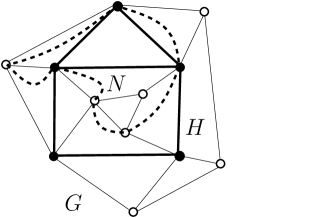
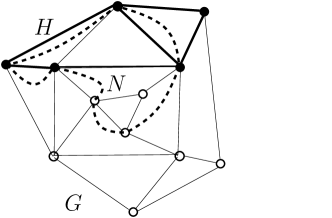
Figure 1: On the left, we have a plane graph $G$ with an emphasized subdrawing $H$ intersected by a combinatorial noose $N$ indicated by dashed lines. On the right, we have the same graph $G$ with a different copy of $H$ intersected by $N$.

The running time of the algorithm crucially depends on the number of combinatorial nooses in $H$. The aim of this section is to prove the following:

Theorem 4.1

Let $G$ be a plane graph on $n$ vertices and $H$ be a plane graph on $k\leq n$ vertices. We can decide if there is a subdrawing of $G$ that is equivalent to $H$ in time $2^{O(k)}n$. We can find and count subdrawings equivalent to $H$ in time $2^{O(k)}n$, and enumerate $\omega$ subdrawings in time $2^{O(k)}n+O(\omega k)$.

4.1 Combinatorial nooses in plane graphs

For a refined algorithm analysis we now take a close look at combinatorial nooses of plane graphs. In particular we are interested in counting the number of combinatorial nooses. In this subsection, we will prove the following lemma:

Lemma 4.2

Every plane $k$-vertex graph has $2^{O(k)}$ combinatorial nooses.

Before proving this lemma, we show that every combinatorial noose of a plane graph on $k$ vertices corresponds to a cycle in some other plane graph on at most $O(k)$ vertices. First we relate combinatorial nooses in a planar triangulation $H^{\prime}$ to the cycles in $H^{\prime}$. In a second step we relate combinatorial nooses of a 3-connected plane graph $H$ to cycles in the triangulations of $H$. Finally, we will show that for any plane graph $H$ there is an auxiliary graph $H^{*}$, such that the combinatorial nooses of $H$ can be injectively mapped to the cycles of the triangulations of $H^{*}$. From Proposition 2.4 we know an upper bound on the number of cycles in planar graphs, which we employ to prove Lemma 4.2.

Lemma 4.3

Let $H$ be a planar triangulation and $N_{C}=[v_{0},f_{0},v_{1},f_{1},\ldots,f_{k-1},v_{k}]$ a combinatorial noose of $H$. Then for every pair of consecutive vertices $v_{i},v_{i+1}$ in $N_{C}$, there is an edge ${v_{i},v_{i+1}}$ in $E(H)$. That is, the sequence $[v_{0},v_{1},\ldots,v_{k}]$ is a simple cycle in $H$ if $|V(N_{C})|>2$, and if $|V(N_{C})|=2$, it corresponds to a single edge in $H$.

Proof.

Since $H$ is triangulated, we have that every $f_{i}\in N_{C}$ is bounded by a triangle $\Delta$ where $v_{i},v_{i+1}$ are two of the three vertices of $\Delta$ and $v_{i},v_{i+1}$ have an edge in common. Since vertices occur only once in $N_{C}$, $f_{i}$ is unique in $N_{C}$ if $|V(N_{C})|>2$, that is, there is no $f_{j}\in N_{C}$ with $i\neq j$ and $f_{i}=f_{j}$. Hence we map each $f_{i}$ one-to-one to edge $e_{i}=\{v_{i},v_{i+1}\}$ and get a cycle $[v_{0},e_{0},v_{1},e_{1},\ldots,e_{k-1},v_{k}]$. For $|V(N_{C})|=2$, $f_{0}$ and $f_{1}$ are incident faces to edge $\{v_{0},v_{1}\}$. For an illustration, see Figure 2.

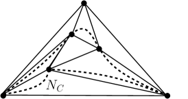
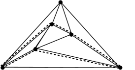
Figure 2: On the left, there is a triangulation with a combinatorial noose $N_{C}$ indicated by dashed lines. On the right, we have mapped the noose to a cycle indicated by dashed lines.

∎

Lemma 4.4

Let $H$ be a 3-connected plane graph and $N_{C}=[v_{0},f_{0},v_{1},f_{1},\ldots,f_{k-1},v_{k}]$ a combinatorial noose of $H$ with $|V(N_{C})|>2$. Then there exists a planar triangulation $H^{\prime}$ of $H$, such that $[v_{0},v_{1},\ldots,v_{k}]$ is a cycle in $H^{\prime}$.

Proof.

We proceed in two phases. First we iteratively add edges to $H$ and transform $N_{C}$ into another combinatorial noose such that every two consecutive vertices in $N_{C}$ have a common edge. Then we triangulate the resulting graph.

For every pair of consecutive vertices $v_{i},v_{i+1}$ in $N_{C}$, if $v_{i},v_{i+1}$ have no edge in common, add $e_{i}=\{v_{i},v_{i+1}\}$ to $E(H)$. Thereby the drawing of $e_{i}$ splits $f_{i}$ into two new faces $f^{a}_{i}$ and $f^{b}_{i}$, bounded by face-cycle $C^{a}$ and $C^{b}$ respectively, where $C^{a}\cap C^{b}=e_{i}$.Since $N_{C}$ corresponds to a noose by Remark 2.3 and nooses are not self-intersecting, we observe the following for $|V(N_{C})|>2$: for every $f_{j}=f_{i}$ in $N_{C}$ with $j\neq i$ we have that both $v_{j},v_{j+1}$ are in one of $C_{a}$ and $C_{b}$. Thus, adding edge $e_{i}$ will not cross any other edge added in this process. In $N_{C}$, we replace $f_{i}$ by one of $f^{a}_{i}$ and $f^{b}_{i}$, and every $f_{j}=f_{i}$ by $f^{a}_{i}$ if $F_{j}$ is bounded by $C^{a}$ and by $f^{b}_{i}$ otherwise. Once we have an edge for every pair of consecutive vertices in $N_{C}$, we note that for every sub-sequence $[v_{i},f_{i},v_{i+1}]$ of $N_{C}$ the edge $e_{i}=\{v_{i},v_{i+1}\}$ is incident to face $f_{i}$ since, by 3-connectivity, edge $e_{i}$ is uniquely embedded in $H$. We then add edges arbitrarily to obtain a triangulation $H^{\prime}$. By Lemma 4.3, the vertices of $N_{C}$ correspond to a cycle in $H^{\prime}$. For an illustration, see Figure 3.

Figure 3: One the left, we see a face of our plane graph with a combinatorial noose $N_{C}$ indicated with dashed lines. To the right, we have mapped the noose to a cycle indicated with dashed lines and dotted lines indicating the face triangulation.

∎

If $H$ is not 3-connected, a problem may occur in the last step of the previous proof when triangulating $H$. Consider a sub-sequence $[v_{i},f_{i},v_{i+1}]$ in $N_{C}$. We assume there already exists an edge $e_{i}=\{v_{i},v_{i+1}\}$ and $v_{i},v_{i+1}$ separate $H$, that is, $H$ is 2-connected. Then it may be the case that $e_{i}$ is not incident to $f_{i}$, and thus, any triangulation of $H$ has an edge crossing $N_{C}$. We surpass this problem in the general case by triangulating some auxiliary graph instead. For an edge $e=\{v,w\}$ of a graph $H$ we subdivide $e$ by adding a vertex $u$ to $V(H)$ and replacing $e$ by two new edges $e_{1}=\{v,u\}$ and $e_{2}=\{u,w\}$. In a drawing of $H$, we place point $u$ in the middle of the drawing of $e$ partitioning $e$ into $e_{1}$ and $e_{2}$.

Lemma 4.5

Let $H$ be plane graph and $N_{C}=[v_{0},f_{0},v_{1},f_{1},\ldots,f_{k-1},v_{k}]$ a combinatorial noose of $H$ with $|V(N_{C})|>2$. Let $H^{*}$ be obtained by subdividing every edge in $E(H)$. There exists a planar triangulation $H^{\prime}$ of $H^{*}$ such that $[v_{0},v_{1},\ldots,v_{k}]$ is a cycle in $H^{\prime}$.

Proof.

The combinatorial noose $N_{C}$ is a combinatorial noose in $H^{*}$, too. As for any two consecutive vertices $v_{i},v_{i+1}$ in $N_{C}$ there is no edge in $H^{*}$ and each vertex in $N_{C}$ is unique, we may add edges to $H^{*}$ as in the proof of Lemma 4.4 and triangulate $H^{*}$. ∎

Proof of Lemma 4.2.

If $H$ is triangulated, we have with Lemma 4.3 that every combinatorial noose corresponds to a unique cycle in $H$. By Proposition 2.4, the number of cycles in $H$ is bounded by $2^{1.53k}$. Since for every edge of a cycle in $H$, we have two choices for a combinatorial noose to visit an incident face, we get the overall upper bound of $2^{2.53k}$ on the number of combinatorial nooses. If $H$ is plane, we have to count the triangulations either of $H$ (Lemma 4.4) or of $H^{*}$ (Lemma 4.5). By Proposition 2.5 and the comments below it, there are at most $2^{3.24\ell}$ non-isomorphic triangulations on $\ell$ vertices. Let us denote this set of triangulated graphs by $\Phi$. We note that $H$ (resp. $H^{*}$) is a subgraph of some graph of $\Phi$, say of all graphs in $\Phi_{H}\subseteq\Phi$ with $|\Phi_{H}|\geq 1$. Since every triangulated graph is 3-connected, we have with Theorem 2.1 that every graph $H^{\prime}$ in $\Phi_{H}$ has a unique embedding in $\Sigma$ up to homeomorphism. The plane graph $H$ (resp. $H^{*}$) is then a subdrawing of a drawing equivalent to an arbitrary plane embedding of $H^{\prime}$ in $\Sigma$. Thus, the number of triangulations times the number of combinatorial nooses in each triangulation is an upper bound on the number of combinatorial nooses in $H$, here $2^{5.77k}$ (resp. in $H^{*}$, here $2^{9.77k}$). ∎

For embedded dynamic programming on a sc-decomposition $\langle T,\mu,\pi\rangle$, we can argue with Remark 2.2 that if $H$ is a subdrawing of $G$, then noose $N$ formed by the middle set $\operatorname{mid}(e)$ is a noose of $H$, too. Recalling Remark 2.3, the alternating sequence of vertices and faces of $H$ visited by $N$ forms a combinatorial noose $N_{C}$ in $H$.

This observation allows us to discuss the results from a combinatorial point of view without the underlying topological arguments. Instead of nooses we will refer to combinatorial nooses in the remaining section.

4.2 Embedded dynamic programming

In embedded dynamic programming, the basic difference to usual dynamic programming is that we do not check for every partial solution for a given problem if or how it lies in the graph processed so far. Instead, we check how the graph that we have processed so far is intersecting the entire solution, that is how the graph is embedded into our solution. For subgraph isomorphism, we compute every possible way the processed subdrawing $G_{sub}$ of $G$ is embedded in the plane pattern $H$ up to homeomorphism, subject to how the bound of $G_{sub}$ intersects $H$. This bound is a combinatorial noose $N$ separating $G_{sub}$ from the rest of $G$. The number of solutions we get is bounded by the number of combinatorial nooses in $H$ we can map $N$ onto.We describe the algorithm in what follows.

Dynamic programming.

We root sc-decomposition $\langle T,\mu,\pi\rangle$ at some node $r\in V(T)$. For each edge $e\in T$, let $L_{e}$ be the set of leaves of the subtree rooted at $e$. The subgraph $G_{e}$ of $G$ is induced by the edge set $\{\mu(v)\mid v\in L_{e}\}$. The vertices of $\operatorname{mid}(e)$ form a combinatorial noose $N$ that separates $G_{e}$ from the residual graph.

Assuming $H$ is a subdrawing of $G$, the basic idea of embedded dynamic programming is that we are interested in how the vertices of the combinatorial noose $N$ are intersecting faces and vertices of $H$. Since every noose in $G$ is a noose in $H$, we can map $N$ to a combinatorial noose $N^{H}$ of $H$, bounding (clockwise) a unique subgraph $H_{sub}$ of $H$.

In each step of the algorithm, all solutions for a sub-problem in $G_{e}$ are computed, namely all possibilities of how $N$ is mapped onto a combinatorial noose $N^{H}$ in $H$ that separates $H_{sub}$ from the rest of $H$, where $H_{sub}\subseteq H$ is isomorphic to subgraphs of $G_{e}$. For every middle set, we store this information in an array. It is updated in a bottom-up process starting at the leaves of $\langle T,\mu,\pi\rangle$. During this updating process it is guaranteed that the ‘local’ solutions for each subgraph associated with a middle set of the sc-decomposition are combined into a ‘global’ solution for the overall graph $G$.

Step 0: Initializing the middle sets.

Let $G$ be a plane graph with a rooted sc-decomposition $\langle T,\mu,\pi\rangle$ and let $H$ be a plane pattern. For every middle set $\operatorname{mid}(e)$ of $\langle T,\mu,\pi\rangle$ let $N$ be the associated combinatorial noose in $G$ with face-vertex sequence of $F(N)\cup V(N)$. Let $\mathfrak{L}$ denote the set of all combinatorial nooses of $H$ whose length is at most the length of $N$. We now want to map $N$ order preserving to each $N^{H}\in\mathfrak{L}$. We map vertices of $N$ to both vertices and faces of $H$. Therefore, we consider partitions of $V(N)=V_{1}(N)\dot{\cup}V_{2}(N)$ where vertices in $V_{1}(N)$ are mapped to vertices of $V(H)$ and vertices in $V_{2}(N)$ to faces of $F(H)$. We define a mapping $\gamma:V(N)\cup F(N)\rightarrow V(H)\cup F(H)$ relating $N$ to the combinatorial nooses in $\mathfrak{L}$. For every $N^{H}\in\mathfrak{L}$ on faces and vertices of set $F(N^{H})\cup V(N^{H})$ and for every partition $V_{1}(N)\dot{\cup}V_{2}(N)$ of $V(N)$ mapping $\gamma$ is valid if

• $\gamma$ restricted to $V_{1}(N)$ is a bijection to $V(N^{H})$;

• for every $v\in V_{1}(N)$ we have $\gamma(v)\in V(N^{H})$, and for every $v\in V_{2}(N)$ we have $\gamma(v)\in F(N^{H})$;

• for every $f\in F(N)$ we have $\gamma(f)\in F(N^{H})$;

• for every pair $v_{h},v_{j}\in V(N)$ such that $[\gamma(v_{h}),f,\gamma(v_{j})]$ is a subsequence of $N^{H}$ for a face $f\in F(N^{H})$ and for every vertex $v_{i}\in V(N)$ with $v_{i}$ lying inbetween $v_{h}$ and $v_{j}$ in the sequence $N$, we have $\gamma(v_{i})=f$;

• for every $v_{i}\in V(N)$ and subsequence $[f_{i-1},v_{i},f_{i}]$ of $N$, if $\gamma(v_{i})\in F(N^{H})$, we have $\gamma(f_{i-1})=\gamma(v_{i})=\gamma(f_{i})$;

• for every pair of vertices $w_{i},w_{j}$ in $V(N^{H})$: if $\{w_{i},w_{j}\}\in E(H)$ then $\{\gamma^{-1}(w_{i}),\gamma^{-1}(w_{j})\}\in E(G)$.

Items $a)$ to $c)$ say where to map the faces and vertices of $N$ to. Items $d)$ and $e)$ make sure that if two vertices $v_{h},v_{j}$ in sequence $N=[\ldots,v_{h},\underline{\ldots},v_{j},\ldots]$ are mapped to two vertices $w_{i},w_{i+1}$ that appear in sequence $N^{H}$ as $[\ldots,w_{i},f_{i},w_{i+1},\ldots]$ then every face and vertex inbetween $v_{h},v_{j}$ in sequence $N$ (here underlined) is mapped to face $f_{i}$. Item $f)$ rules out the invalid solutions, that is, we do not map a pair of vertices in $G$ that have no edge in common to the endpoints of an edge in $H$. We do so because if $H$ is a subdrawing of $G$ then an edge in $H$ is an edge in $G$, too. For an illustration, see Figure 4.

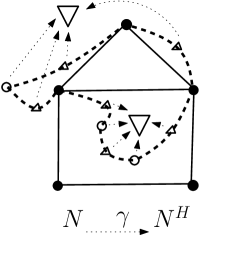
Figure 4: On the left, we have a plane graph $G$ with a subdrawing $H$ emphasized. A combinatorial noose $N$ separating subgraph $G_{e}$ is indicated by dashed lines. The vertices of $N$ are full and empty circles and the faces triangles. In the middle, we have $H$ and indicate to which faces (big triangles) of $H$ vertices and faces of $N$ are mapped by $\gamma$. This gives us combinatorial noose $N^{H}$ on the right, separating subgraph $H_{sub}$.

We assign an array $A_{e}$ to each $\operatorname{mid}(e)$ consisting of all tuples $\langle N^{H},\gamma(N)\rangle$ each representing a valid mapping $\gamma(N)$ from combinatorial noose $N$ corresponding to $\operatorname{mid}(e)$ to a combinatorial noose $N^{H}\in\mathfrak{L}$. The vertices and faces of $N$ are oriented clockwise around $G_{e}$. Without loss of generality, we assume for every $\langle N^{H},\gamma(N)\rangle\in A_{e}$ the orientation of $N^{H}$ to be clockwise around the subgraph $H_{sub}$ of $H$ isomorphic to a subgraph of $G_{e}$.

Step 1: Update process.

We update the arrays of the middle sets in post-order manner from the leaves of $T$ to root $r$. In each dynamic programming step, we compare the arrays of two middle sets $\operatorname{mid}(e),\operatorname{mid}(f)$ in order to create a new array assigned to the middle set $\operatorname{mid}(g)$, where $e,f$ and $g$ have a vertex of $T$ in common. From [12] we know about a special property of sc-decompositions: namely that the combinatorial noose $N_{g}$ is formed by the symmetric difference of the combinatorial nooses $N_{e},N_{f}$ and that $G_{g}=G_{e}\cup G_{f}$. In other words, we are ensured that if two solutions on $G_{e}$ and $G_{f}$ bounded by $N_{e}$ and $N_{f}$ fit together, then they form a new solution on $G_{g}$ bounded by $N_{g}$. We now determine when two solutions represented as tuples in the arrays $A_{e}$ and $A_{f}$ fit together. We update two tuples $\langle N^{H}_{e},\gamma_{e}(N_{e})\rangle\in A_{e}$ and $\langle N^{H}_{f},\gamma_{f}(N_{f})\rangle\in A_{f}$ to a new tuple in $A_{g}$ if

• for all $v\in V(N_{e})\cap V(N_{f})$, $\gamma_{e}(v)=\gamma_{f}(v)$;

• for all $f\in F(N_{e})\cap F(N_{f})$, $\gamma_{e}(f)=\gamma_{f}(f)$;

• for the subgraph $H_{e}$ of $H$ separated by $N^{H}_{e}$ and the subgraph $H_{f}$ of $H$ separated by $N^{H}_{f}$, we have that $E(H_{e})\cap E(H_{f})=\emptyset$ and $V(H_{e})\cap V(H_{f})\subseteq\{\gamma(v)\mid v\in V(N_{e})\cap V(N_{f})\}$.

If $N_{e}$ and $N_{f}$ fit together, we get a valid mapping $\gamma_{g}:N_{g}\rightarrow N^{H}_{g}$ as follows:

• for every $x\in(\,V(N_{e})\cup F(N_{e})\,)\cap(\,V(N_{f})\cup F(N_{f})\,)\cap(\,V(N_{g})\cup F(N_{g}),)$ we have $\gamma_{e}(x)=\gamma_{f}(x)=\gamma_{g}(x)$;

• for every $y\in(\,V(N_{e})\cup F(N_{e})\,)\setminus(\,V(N_{f})\cup F(N_{f})\,)$ we have $\gamma_{e}(y)=\gamma_{g}(y)$;

• for every $z\in(\,V(N_{f})\cup F(N_{f})\,)\setminus(\,V(N_{e})\cup F(N_{e})\,)$ we have $\gamma_{f}(z)=\gamma_{g}(z)$.

We have that $\gamma_{g}$ is a valid mapping from $N_{g}$ to the combinatorial noose $N^{H}_{g}$ that bounds subgraph $H_{g}=H_{e}\cup H_{f}$. Thus, we add tuple $\langle N^{H}_{g},\gamma_{g}(N_{g})\rangle$ to array $A_{g}$.

Step 2: End of DP

If, at some step, we have a solution where the entire subgraph $H$ is formed, we exit the algorithm confirming. That is, if $H=H_{e}\cup H_{f}$ and $H_{i}$ is bounded by $N_{i}$ (for both $i\in\{e,f\}$) then the combinatorial noose $N_{g}$ is bounding the subgraph of $G$ isomorphic to $H$. We are able to output this subgraph by reconstructing the solution top-down in $\langle T,\mu,\pi\rangle$. If at root $r$ no subgraph isomorphic to $H$ has been found, we output ’FALSE’.

Correctness of DP

Let plane graph $H$ be a subdrawing of $G$. We have seen already in Step 0 how we map every combinatorial noose of $G$ that identifies a separation of $G$ via a valid mapping $\gamma$ to a combinatorial noose of $H$ determining a separation of $H$. Every edge of $H$ is bounded by a combinatorial noose $N^{H}$ of length two, which is determined by tuple $\langle N^{H},\gamma(N)\rangle$ in an array assigned to a leaf edge of $T$. We need to show that Step 1 computes a valid solution for $N_{g}$ from $N_{e}$ and $N_{f}$ for incident edges $e,f,g$. We note that the property that the symmetric difference of the combinatorial nooses $N_{e}$ and $N_{f}$ forms a new combinatorial noose $N_{g}$ is passed on to the combinatorial nooses $N^{H}_{e},N^{H}_{f}$ and $N^{H}_{g}$ of $H$, too. If the two solutions fit together, then $H_{e}$ of $H$ separated by $N^{H}_{e}$ and subgraph $H_{f}$ of $H$ separated by $N^{H}_{f}$ only intersect in the image of $V(N_{e})\cap V(N_{f})$. We may observe that $N^{H}_{e}$ and $N^{H}_{f}$ intersect in a continuous alternating subsequence with order reversed to each other, i.e., $N^{H}_{e}\mid_{N_{e}\cap N_{f}}=\overline{N^{H}_{f}}\mid_{N_{e}\cap N_{f}}$, where $\overline{N^{H}}$ means the reversed sequence $N^{H}$. Since every oriented $N^{H}$ identifies uniquely a separation of $E(H)$, we can easily determine if two tuples $\langle N^{H}_{e},\gamma_{e}(N_{e})\rangle\in A_{e}$ and $\langle N^{H}_{f},\gamma_{f}(N_{f})\rangle\in A_{f}$ fit together and form a new subgraph of $H$. If $H$ is a subdrawing of $G$, then at some step we will enter Step 2 and produce the entire $H$.

Running time analysis.

We first give an upper bound on the size of each array. The number of combinatorial nooses in $\mathfrak{L}$ we are considering is bounded by the total number of combinatorial nooses in $H$, which is $2^{O(|V(H)|)}$ by Lemma 4.2. The number of partitions of vertices of any combinatorial noose $N$ is bounded by $2^{|V(N)|}$. Since the order of both $N^{H}$ and $N$ is given we only have $2|V(H)|$ possibilities to map vertices of $N$ to $N^{H}$, once the vertices of $N$ are partitioned. Thus, in an array $A_{e}$ we may have up to $2^{O(|V(H)|)}\cdot 2^{|V(N)|}\cdot|V(H)|$ tuples $\langle N^{H}_{e},\gamma(N_{e})\rangle$. We first create all tuples in the arrays assigned to the leaves. Since middle sets of leaves only consist of an edge in $G$, we get arrays of size $O(|V(H)|^{2})$ which we compute in the same asymptotic running time. When updating middle sets $\operatorname{mid}(e),\operatorname{mid}(f)$, we compare every tuple of one array $A_{e}$ to every tuple in array $A_{f}$ to check if two tuples fit together. We can compute the unique subgraph $H_{e}$ (resp. $H_{f}$) described by a tuple in $A_{e}$ (resp. $A_{f}$), compare two tuples in $A_{e},A_{f}$ and create a new tuple in $A_{g}$ in time linear in the order of $V(N)$ and $V(H)$. Since the size of $A_{g}$ is bounded by $2^{O(|V(H)|)}\cdot 2^{O(|V(N)|)}$, the update process for two middle sets takes the same asymptotic time. Assuming sc-decomposition $\langle T,\mu,\pi\rangle$ of $G$ has width $\omega$ and $|V(H)|\leq\omega$, we get the following result.

Lemma 4.6

For a plane graph $G$ with a given sc-decomposition $\langle T,\mu,\pi\rangle$ of $G$ of width $w$ and a plane pattern $H$ on $k\leq w$ vertices we can search for a subdrawing of $G$ equivalent to $H$ in time $2^{O(w)}\cdot n$.

4.3 The algorithm

We present the overall algorithm for solving Plane Subgraph Isomorphism with running time stated in Theorem 4.1.

Input : Plane graph $G$; Plane pattern $H$ of order $k$.

Choose an arbitrary vertex $v$ in $G$.

Partition $V(G)$ into $S_{0}\cup S_{1}\cup\ldots\cup S_{\ell}$ with $S_{i}=\{w\in V(G):\mbox{dist}(v,w)=i\}$

for every $G_{i}=G[S_{i}\cup\ldots\cup S_{i+k}]$ with $0\leq i\leq\ell-k$ do  Compute sc-decomposition $\langle T,\mu,\pi\rangle$ of $G_{i}$.

Do embedded dynamic programming on $\langle T,\mu,\pi\rangle$ to find a subgraph of $G_{i}$ isomorphic to $H$ and intersecting $S_{i}$.

 

Algorithm 4.1 Plane subgraph isomorphism: PLSI.

5

5

5

5

5

Partitioning the vertex set in Line 4.1 of Algorithm 4.1 PLSI, is a similar approach to the well-known Baker-approach [2]. Every vertex set $S_{i}$ contains the vertices of distance $i$ to the chosen vertex $v$. $S_{0}=\{v\}$ and $\ell$ is the maximum distance in $G$ from $v$. The graph $G_{i}$ in Line 4.1 is induced by the sets $S_{i},\ldots,S_{i+k}$. As in [14], we may argue that every vertex in $G$ appears in at most $k$ subgraphs $G_{i}$. This keeps our running time linear in $n$. We can apply Lemma 3.1 to each $G_{i}$ in Line 4.1 to a compute sc-decomposition $\langle T,\mu,\pi\rangle$ of width $\leq 2k$, by adding a root vertex $r$ for the BFS tree and make $r$ adjacent to every vertex in $S_{i}$. The dynamic programming approach can easily be turned into an algorithm counting subgraph isomorphisms (similar to [14]), by using a counter in the dynamic programming. Using an inductive argument, for every subgraph $G_{i}$ in Line 4.1 we only compute subgraphs intersecting with vertices in $S_{i}$ and thus omit double-counting. We can also adopt our technique to list the subgraphs of $G$ isomorphic to $H$.

5 Planar subgraph isomorphism

Now we consider the case when both pattern $H$ and host graph $G$ are planar but not embedded. However, we observe that if $H$ is isomorphic to a subgraph of $G$, then for every planar embedding of $G$ there exists a drawing of $H$ that is equivalent to a subdrawing of $G$. Hence, we may simply embed $G$ planarly, and run the algorithm of the previous section for all non-equivalent embeddings of $H$. The following lemma tells us that the number of times we call the algorithm is restricted, too.

Lemma 5.1

Every planar $k$-vertex graph has $2^{O(k)}$ non-equivalent embeddings in $\Sigma$.

Proof.

By Proposition 2.5, there are at most $2^{3.24k}$ non-isomorphic maximal planar graphs on $k$ vertices. Every planar graph $H$ is a subgraph of a maximal planar graph. Every maximal planar graph has a unique embedding which is a triangulation. Thus, every embedding of $H$ is a subdrawing of a triangulation of $H$. The number of such subgraphs is bounded by the number of edge subsets of $H^{\prime}$, since for every edge subset of $S\subseteq E(H^{\prime})$ of same cardinality as $E(H)$, $H^{\prime}[S]$ may be isomorphic to $H$. In this case, $H^{\prime}[S]$ then gives a possible embedding of $H$ in $\Sigma$. Hence, the number of embeddings of $H$ in $\Sigma$ up to homeomorphism is bounded by $2^{6.24k}$. ∎

The whole algorithm

Input : Planar graph $G$, Planar pattern $H$ of size $k$.

Compute a planar embedding of $G$.

if $H$ triangulated or 3-connected then Return PLSI$(G,H)$.

for every non-equivalent embedding $I$ of $H$ do  Return PLSI$(G,I)$.  

Algorithm 5.1 Planar subgraph isomorphism.

We compute in Algorithm 5.1 every non-equivalent embedding of $H$ using the constructive proof of Lemma 5.1. That is, we compute the set $\mathcal{H}$ of non-isomorphic maximal planar graphs in time proportional to its size using the algorithm in [20]. For every graph $H^{\prime}\in\mathcal{H}$ and every subdrawing $I$ of $H^{\prime}$ we check whether $I$ is isomorphic to $H$ by using the linear time algorithm for planar graph isomorphism in [19] . By Lemma 5.1, we then call Algorithm 4.1 $2^{O(k)}$ times, for each plane drawing $I$ isomorphic to $H$. This ensures us that Algorithm 5.1 has running time as stated in Theorem 1.1.

6 Conclusion

We have shown how to use topological graph theory to improve the results on the already mentioned variations of Planar Subgraph Isomorphism, solving the open problems posed in [14] and [12]. With the results of [15], [14] extends the feasible graph class from planar graphs to apex-minor-free graphs. This cannot be done with the tools presented here. However, [11] devise a truly subexponential algorithm for $k$-Longest Path in $H$-minor-free graphs and thus apex-minor-free graphs, employing the structural theorem of Robertson and Seymour [24] and the results of [8, 5, 9]. Can the structure of $H$-minor-free graphs, be exploited for our purposes?

It seems unlikely that our work can be extended to obtain a subexponential algorithm. The first reason, mentioned in the introduction, is that Bidimensionality applies to subgraphs with minor properties rather than to general subgraphs. Secondly, our enumerative bounds are either tight or of lower bound $2^{\Omega(k)}$. We want to pose the open problem: Is Plane Subgraph Isomorphism solvable in time $2^{o(k)}n^{O(1)}$?

Acknowledgments. The author thanks Paul Bonsma, Holger Dell and Fedor Fomin for discussions and comments of great value to the presentation of these results.

Appendix A SC-Decompositions in linear time

For a plane graph $G$ we define a radial graph $R_{G}$ as follows: $R_{G}$ is a bipartite graph with the bipartition $F(G)\cup V(G)$. A vertex $v\in V(G)$ is adjacent in $R_{G}$ to a vertex $f\in F(G)$ if and only if the vertex $v$ is incident to the face $f$ in the drawing of $G$.

Let $G$ be a plane graph with some vertex $r\in V(G)$ and $R_{G}$ its radial graph. Let $T$ be a spanning tree of $G$ rooted at $f$ that is determined by breadth first search. Choose a face $f$ adjacent to root $r$. If the longest path from $r$ to a leaf of $T$ is $\ell$ then the distance $d_{f}$ in the radial graph $R_{G}$ from vertex $f$ to any other (face)vertex $x$ is at most $2\ell+1$. This is due to the fact that there exists an edge $\{f,r\}$ in $R_{G}$, and for every edge in $T$ there is a detour in $R_{G}$ of at most two edges. [25] show how to obtain a branch decomposition of width $d_{f}$ out of a BFS spanning tree rooted at $r$ of the radial graph. Set $f$ to be the outer face of $G$. Let $T$ be a BFS spanning tree of $R_{G}$ rooted at $f$ and let $\ell$ be the maximum distance in $T$ from $r$ to a leaf. We give now a compact presentation of the algorithm of [25] and show that it translates to constructing a sphere-cut decomposition of $G$.We define contracting a vertex $v$ as identifying all vertices of $N(v)$ to a single vertex and deleting $v$.

Input :  Plane graph $G$, face $f\in F(G)$ , radial graph $R_{G}$ .

Output : Branch-decomposition of $G$ of width at most $2\ell+1$.

Construct embedded BFS tree $T_{S}$ of $R_{G}$ at root $f$.

Set $T^{*}=R_{G}^{*}\setminus E(T_{S})^{*}$ the dual graph of $R_{G}$ without the edge set dual to $T_{S}$

for every node $v$ in $T^{*}$ do  if $\deg(v)_{T}=1$ then

 create $C_{v}$ a single edge, with nodes labeled $\{v\}$ and $\{N(v)\}$;

else 

 create embedded ternary tree $C_{v}$ with $|N(v)|+1$ leaves;

 label one leaf with $\{v\}$ and the other leaves with $N(v)$ keeping a clockwise order.

 

(in post order) for every edge $\{u,v\}$ in $T^{*}$, where $v$ is the parent node do  combine $C_{u}$ and $C_{v}$ by identifying leaf $\{v\}$ in $C_{u}$ with leaf $\{u\}$ in $C_{v}$, and

 contract the identified node and set new tree to be named $C_{v}$. 

Return ($C_{r}$ (for $r$ root of $T^{*}$)).

Algorithm A.1 Computing SC-decomposition.

12

12

12

12

12

12

12

12

12

12

12

12

In [25], Algorithm A.1 is proved to compute a branch decomposition of planar graph $G$ of width $2\ell+1$ in time $O(\ell n)$.

Claim A.1

Algorithm A.1 computes a sc-decomposition of $G$.

Proof.

Observe that the edge set $T^{*}$ of the dual graph of $R_{G}$ (the so-called medial graph) minus the dual edges of $T_{S}$ in Line A.1 forms a tree due to the acyclicity of $T_{S}$. Every node of $T^{*}$ corresponds to an edge of $G$ and in fact, spans the edge set of $G$. For turning $T^{*}$ into a branch-decomposition we $a)$ bijectively map the leafs of $T^{*}$ to the edges of $G$ and $b)$ make $T^{*}$ ternary. For $a)$ we generate for every node $v$ in $T^{*}$ from Line A.1–A.1 one ternary tree (or single edge tree), a local tree $C_{v}$ with $v$ one leaf. In Line A.1–A.1 those local trees are merged from the leaves of $T^{*}$ to its root in post order such that each $C_{v}$ contributes to leaf $v$ in the overall ternary tree $C_{r}$. We show now that the such formed branch decomposition actually obeys our definition of an sc-decomposition, that is the vertices in each middle set form a cycle in the radial graph. Note that every edge of $G$ forms a $4$-cycle in $R_{G}$. Let $e^{*}\in E(T^{*})$ be the dual edge of edge $e=\{f,g\}\in E(R_{G}\setminus T_{S})$. Then the union of $e$ and the path through $T_{S}$ from $f$ over the lowest common ancestor of $f,g$ in $T_{S}$ to $g$ forms a cycle in $R_{G}$ that separates the two subtrees of $T^{*}$ that are separated by $e^{*}$. Thus, $T^{*}$ already possesses middle sets that form nooses in $G$. However $T^{*}$ is not ternary since it may have maximum node degree $4$. The leaves of each local tree $C_{v}$ in Line A.1 are embedded in the same order as the inverse of their labels, the neighboring nodes of $v$ in $T^{*}$, and thus we keep the same ordering in the overall ternary tree $C_{r}$. Every edge $e$ of $C_{r}$ comes from an edge of one of the local trees $C_{v}$, and $e$ separates the neighbors $N_{1}(v)$ from $N_{2}(v)$ where the disjoint union $N_{1}(v),N_{2}(v)$ form the neighborhood $N(v)$ of $v$ in $T^{*}$. Like this, $T^{*}$ falls apart into two subtrees each bounded by a cycle in $R_{G}$ formed similarly as above by the union of $N_{i}(v)$ bounding minimal path in $T_{S}$ and the path through the edges of $T^{*}$ induced by $N_{i}[v]$, for $i=1$ and $i=2$ respectively.

∎

References

- [1] N. Alon, R. Yuster, and U. Zwick, Color-coding, J. Assoc. Comput. Mach., 42 (1995), pp. 844–856.
- [2] B. S. Baker, Approximation algorithms for NP-complete problems on planar graphs, J. Assoc. Comput. Mach., 41 (1994), pp. 153–180.
- [3] H. L. Bodlaender, A linear-time algorithm for finding tree-decompositions of small treewidth, SIAM J. Comput., 25 (1996), pp. 1305–1317.
- [4] K. Buchin, C. Knauer, K. Kriegel, A. Schulz, and R. Seidel, On the number of cycles in planar graphs, in Proceedings of the 13th Annual International Conference on Computing and Combinatorics (COCOON’07), vol. 4598 of Lecture Notes in Computer Science, Springer, 2007, pp. 97–107.
- [5] A. Dawar, M. Grohe, and S. Kreutzer, Locally excluding a minor, in Proceedings of the 22nd IEEE Symposium on Logic in Computer Science (LICS 2007), IEEE Computer Society, 2007, pp. 270–279.
- [6] E. D. Demaine, F. V. Fomin, M. T. Hajiaghayi, and D. M. Thilikos, Subexponential parameterized algorithms on graphs of bounded genus and -minor-free graphs, Journal of the ACM, 52 (2005), pp. 866–893.
- [7] E. D. Demaine and M. T. Hajiaghayi, The bidimensionality theory and its algorithmic applications, Computer Journal, 51 (2008), pp. 292–302.
- [8] E. D. Demaine, M. T. Hajiaghayi, and K. Kawarabayashi, Algorithmic graph minor theory: Decomposition, approximation, and coloring, in Proceedings of the 46th Annual IEEE Symposium on Foundations of Computer Science (FOCS 2005), IEEE Computer Society, 2005, pp. 637–646.
- [9] E. D. Demaine, M. T. Hajiaghayi, and D. M. Thilikos, Exponential speedup of fixed-parameter algorithms for classes of graphs excluding single-crossing graphs as minors., Algorithmica, 41 (2005), pp. 245–267.
- [10] R. Diestel, Graph theory, vol. 173 of Graduate Texts in Mathematics, Springer-Verlag, New York, second ed., 2000.
- [11] F. Dorn, F. V. Fomin, and D. M. Thilikos, Catalan structures and dynamic programming on H-minor-free graphs, in Proceedings of the 19th Annual ACM-SIAM Symposium on Discrete Algorithms (SODA 2008), ACM, New York, 2008, pp. 631–640.
- [12] F. Dorn, E. Penninkx, H. L. Bodlaender, and F. V. Fomin, Efficient exact algorithms on planar graphs: Exploiting sphere cut decompositions, Algorithmica, (2009, to appear).
- [13] R. G. Downey and M. R. Fellows, Parameterized complexity, Springer-Verlag, New York, 1999.
- [14] D. Eppstein, Subgraph isomorphism in planar graphs and related problems, Journal of Graph Algorithms and Applications, 3 (1999), pp. 1–27.
- [15] D. Eppstein, Diameter and treewidth in minor-closed graph families, Algorithmica, (2009).
- [16] J. Flum and M. Grohe, Parameterized Complexity Theory, Texts in Theoretical Computer Science. An EATCS Series, Springer-Verlag, Berlin, 2006.
- [17] F. V. Fomin and D. M. Thilikos, New upper bounds on the decomposability of planar graphs, Journal of Graph Theory, 51 (2006), pp. 53–81.
- [18] M. R. Garey and D. S. Johnson, Computers and Intractability, A Guide to the Theory of NP-Completeness, W.H. Freeman and Company, New York, 1979.
- [19] J. E. Hopcroft and J. K. Wong, Linear time algorithm for isomorphism of planar graphs (preliminary report), in Proceedings of the Sixth Annual ACM Symposium on Theory of Computing (STOC’74), ACM, 1974, pp. 172–184.
- [20] Z. Li and S.-I. Nakano, Efficient generation of plane triangulations without repetitions, in Proceedings of the 28th International Colloquium on Automata, Languages and Programming (ICALP’01), vol. 2076 of Lecture Notes in Computer Science, Springer, 2001, pp. 433–443.
- [21] R. Niedermeier, Invitation to fixed-parameter algorithms, vol. 31 of Oxford Lecture Series in Mathematics and its Applications, Oxford University Press, Oxford, 2006.
- [22] J. Plehn and B. Voigt, Finding minimally weighted subgraphs, in Proceedings of the 16th International Workshop on Graph-Theoretic Concepts in Computer Science (WG’90), vol. 484 of Lecture Notes in Computer Science, Springer, 1990, pp. 18–29.
- [23] N. Robertson, P. Seymour, and R. Thomas, Quickly excluding a planar graph, Journal of Combinatorial Theory Series B, 62 (1994), pp. 323–348.
- [24] N. Robertson and P. D. Seymour, Graph minors. XVI. Excluding a non-planar graph, J. Combin. Theory Ser. B, 89 (2003), pp. 43–76.
- [25] H. Tamaki, A linear time heuristic for the branch-decomposition of planar graphs, in Proceedings of the 11th Annual European Symposium on Algorithms (ESA’03), vol. 2832 of Lecture Notes in Computer Science, Springer, 2003, pp. 765–775.
- [26] W. T. Tutte, A census of planar triangulations, Canad. J. Math., 14 (1962), pp. 21–38.