7 mm continuum observations of ultra compact HII regions

Abstract

Aims. Ultra compact HII (UCHII) regions are indicators of high-mass star formation sites and are distributed mainly in the Galactic plane. They exhibit a broad band spectrum with significant emission between near-IR and radio wavelengths. We intend to investigate the possible contribution of the forthcoming ESA Planck mission to the science of UCHII regions by evaluating the possibility of detecting UCHIIs that are bright in the radio regime.

Methods. We performed new 7 mm observations of a sample of UCHII regions. The observations were designed to acquire high-frequency radio spectra. For each source in our sample, the free-free radio spectrum has been modeled. Along with far-IR measurements, our spectra allow us to estimate the flux densities of the sources in the millimeter and sub-millimeter bands. We extrapolated and summed the ionized-gas (free-free radio emission) and dust (thermal emission) contributions in the afore mentioned wavelength ranges. The possibility of Planck detecting the selected sources can be assessed by comparing the estimated flux densities to the expected sensitivity in each Planck channel. To obtain a realistic estimation of the noise produced by the Galactic emission, the Planck sky model software package was used.

Results. For each target source, from our new 7 mm data and other radio measurements from the literature, important physical parameters such as electron density and their spatial distribution, source geometry and emission measure were derived. We conclude that, in the case of the present sample, located close to the Galactic center, Planck will have a very low detection rate. In contrast, assuming that our sample is representative of the whole UCHII-region population, we derive a very high probability of detecting this kind of source with Planck if located instead close to the anticenter. From the analysis of the ionized-gas properties, we suggest that the selected sample could also be contaminated by other kinds of Galactic objects.

1 Introduction

The Planck mission of the European Space Agency (ESA) will operate over a wide range of frequencies, from 30 to 900 GHz (from 1 cm to about 300 $\mu$m). The frequency coverage of the Planck channels was selected to correspond to the so-called cosmic microwave background (CMB) window, where temperature fluctuations due to Galactic emission are minimal. Although Planck was designed for cosmological studies, its multi-frequency nearly-full-sky maps will have a profound impact on fundamental physics as well as Galactic and extragalactic astrophysics and several Galactic projects are indeed included in its core program (see The Planck Collaboration, (2005) for details about the scientific case for the Planck mission).

Table 1: Observations.

MSX6C Name	R.A. (J2000)	Dec. (J2000)	$S_{\mathrm{7}}$	$\sigma_{\mathrm{7}}$	MSX6C Name	R.A. (J2000)	Dec. (J2000)	$S_{\mathrm{7}}$	$\sigma_{\mathrm{7}}$
	[ h m s]	[${}^{\circ}\ {}^{\prime}\ {}^{\prime\prime}$]	[mJy]	[mJy]		[ h m s]	[${}^{\circ}\ {}^{\prime}\ {}^{\prime\prime}$]	[mJy]	[mJy]
$17.2231+0.3952$	18 20 46.13	$-13$ 45 21.4	$595$	$90$	$29.2113-0.0690$	18 44 53.36	$-03$ 20 28.1	$150$	$50$
$16.9440-0.0736^{{\dagger}}$	18 21 56.0	$-14$ 13 28	$770$	$160$	$29.9564-0.0174$	18 46 04.07	$-02$ 39 16.6	$3320$	$300$
$18.4608-0.0034$	18 24 36.34	$-12$ 51 00.0	$330$	$70$	$30.5345+0.0209$	18 46 59.38	$-02$ 07 20.7	$1070$	$100$
$18.7104+0.0001$	18 25 04.15	$-12$ 37 40.1	$270$	$70$	$30.2340-0.1392$	18 47 00.40	$-02$ 27 47.9	$250$	$60$
$18.3029-0.3910^{{\dagger}}$	18 25 42.5	$-13$ 10 20	$1260$	$210$	$30.8667+0.1141$	18 47 15.71	$-01$ 47 05.4	$560$	$110$
$18.7084-0.1263$	18 25 31.45	$-12$ 41 18.5	$240$	$60$	$31.4134+0.3092$	18 47 34.35	$-01$ 12 40.2	$700$	$120$
$19.7403+0.2799$	18 26 01.33	$-11$ 35 08.4	$160$	$40$	$30.6877-0.0729$	18 47 36.01	$-02$ 01 44.4	$880$	$140$
$18.8330-0.3004$	18 26 23.64	$-12$ 39 35.9	$280$	$60$	$30.7206-0.0826$	18 47 41.79	$-02$ 00 18.6	$570$	$130$
$21.8732+0.0076^{{\dagger}}$	18 31 02.4	$-09$ 49 33	$560$	$100$	$31.0702+0.0498$	18 47 51.74	$-01$ 38 00.4	$220$	$60$
$21.3853-0.2537$	18 31 03.90	$-10$ 22 40.7	$215$	$50$	$31.2803+0.0615$	18 48 11.89	$-01$ 26 26.0	$310$	$60$
$22.7253-0.0106$	18 32 41.91	$-09$ 04 40.8	$195$	$50$	$30.6671-0.3316$	18 48 29.24	$-02$ 09 57.0	$205$	$50$
$23.9548+0.1494^{{\dagger}}$	18 34 25.3	$-07$ 54 50	$1170$	$160$	$31.2430-0.1108^{{\dagger}}$	18 48 45.1	$-01$ 33 13	$660$	$110$
$24.5076-0.2222^{{\dagger}}$	18 36 46.9	$-07$ 35 38	$630$	$100$	$32.1514+0.1317^{{\dagger}}$	18 49 32.7	$-00$ 38 04	$680$	$100$
$25.5196+0.2156$	18 37 05.20	$-06$ 29 32.5	$360$	$90$	$31.3948-0.2585$	18 49 33.28	$-01$ 29 07.5	$380$	$90$
$25.2666-0.1584$	18 37 57.97	$-06$ 53 25.9	$220$	$50$	$32.4727+0.2041$	18 49 52.56	$-00$ 18 53.1	$220$	$50$
$25.3977-0.1406^{{\dagger}}$	18 38 08.2	$-06$ 45 57	$2540$	$170$	$32.7977+0.1903$	18 50 30.86	$-00$ 01 52.7	$3800$	$300$
$25.3820-0.1813$	18 38 15.15	$-06$ 47 53.8	$2730$	$300$	$32.2718-0.2260$	18 51 02.37	$-00$ 41 19.9	$280$	$70$
$26.0905-0.0578^{{\dagger}}$	18 39 07.2	$-06$ 06 44	$165$	$50$	$33.8104-0.1869^{{\dagger}}$	18 53 42.4	$+00$ 41 48	$400$	$80$
$26.6085-0.2122$	18 40 37.47	$-05$ 43 15.4	$165$	$50$	$35.4672+0.1381$	18 55 34.11	$+02$ 19 15.7	$350$	$60$
$27.4938+0.1893^{{\dagger}}$	18 40 49.2	$-04$ 45 06	$500$	$60$	$35.5736+0.0678$	18 56 00.96	$+02$ 22 59.2	$300$	$60$
$27.9777+0.0780$	18 42 06.41	$-04$ 22 14.5	$220$	$70$	$35.5789-0.0304$	18 56 22.56	$+02$ 20 32.7	$540$	$90$
$28.2461+0.0134$	18 42 49.66	$-04$ 09 45.7	$185$	$50$	$38.5497+0.1636^{{\dagger}}$	19 01 07.6	$+05$ 04 23	$165$	$40$
$28.2007-0.0494$	18 42 58.12	$-04$ 13 55.7	$980$	$160$	$38.8750+0.3088$	19 01 12.49	$+05$ 25 48.1	$390$	$60$
$28.6096+0.0170^{{\dagger}}$	18 43 28.9	$-03$ 50 18	$420$	$90$	$39.8821-0.3457$	19 05 24.11	$+06$ 01 31.4	$300$	$60$
$28.6520+0.0271$	18 43 31.40	$-03$ 47 40.6	$300$	$70$	$41.7410+0.0972^{{\dagger}}$	19 07 15.5	$+07$ 52 42	$310$	$40$
$28.2875-0.3639$	18 44 15.09	$-04$ 17 51.3	$585$	$120$

• Reported as a multi source in the 6 cm catalog but associated with the same MSX source. The 7 mm observations were carried out by pointing at the MSX coordinates.

In the science of compact Galactic objects, Planck will be sensitive to the millimeter emission from dusty envelopes of young and old stars and to the thermal radio emission from the ionized gas surrounding many classes of stellar objects.

HII regions of size about 0.1 pc, emission measure higher than 10⁷ pc cm^-6, electron density higher than $10^{4}$ cm^-3, and ionized mass of around $10^{-2}$ M_⊙ are classified as ultra compact HII regions (UCHIIs) and are sites of high-mass star formation. In these regions, newly born stars are still embedded in their natal molecular clouds. The ambient dust thermally reradiates the entire luminosity of the central star in the infrared (IR), making UCHIIs among the brightest IR sources in the Galaxy. The radiation fields of the massive hot stars inside UCHIIs (OB spectral type) ionize the circumstellar material. The signature of ionization is the typical free-free flux-density distribution at radio wavelengths ($S_{\nu}\propto\nu^{\alpha}$). Therefore, we expect the Galactic population of UCHIIs to be a strong foreground contamination source to the Planck experiment.

As part of the preparation of a Planck pre-launch catalog, we started an observing program to measure the 7 mm flux density of samples of Galactic sources with the 32 m INAF-IRA Noto Radiotelescope. In a previous paper (Umana et al., 2008a ), we published the our flux density measurements of planetary nebulae (PNe).

In this paper, we present new 7 mm single-dish observations of UCHIIs. Main goal was to obtain reliable estimates of the flux densities expected in Planck channels by building and modeling the spectral energy distribution (SED) of our targets. The observing frequency (43 GHz) is within the cosmic microwave background (CMB) window and represents one of the channels of the forthcoming Planck mission. Therefore, in this frequency band, we obtain a direct measurement of the expected flux density with minimal frequency extrapolation.

As added value, the present work provides a sizeable dataset of 7 mm measurements of UCHII regions. These data provide strong constraints on the observed SEDs in the spectral region where free-free emission dominates.

The SED modeling in the radio-millimeter spectral range is a crucial step for the study of the physics of ionized envelopes around UCHII regions. The 7 mm measurements presented in this paper provide the possibility of constraining parameters such as the electron density and the radial profile, the source geometry, and the emission measure.

2 Sample selection

Our sample was selected from the catalog of Giveon et al., 2005a , where a cross-correlation between the Midcourse Space Experiment (MSX6C) catalog (Egan et al., 2003) and the Multi-Array Galactic Plane Imaging Survey (MAGPIS) (White et al., 2005) was performed. MAGPIS was carried out at 6 cm and covered Galactic regions with longitude $350^{\circ}\leq l\leq 42^{\circ}$ and latitude $|b|\leq 0.4^{\circ}$. A comparison of the two catalogs (radio and infrared) allowed the authors to find a sample of 687 radio sources with highly-reliable infrared counterparts. Only 228 of 687 targets were detected in the new MAGPIS at 20 cm (Helfand et al., 2006).

All sources with both 6 and 20 cm data have red MSX colors and flat or inverted spectral indices, as is typical of thermal radio sources. The average spectral index between 20 and 6 cm is equal to 0.28. Giveon et al., 2005a classified these sources as compact HII regions on the basis of their radio and infrared properties. For most sources, this was their first classification. Starting from this subsample of 228, we first inspected all the corresponding MAGPIS 6 cm images.

To minimize the source-structure effect on the flux density measurements, we selected only sources compact enough to be considered point-like at the resolution of the Noto Radiotelescope at 7 mm (HPBW about $1^{\prime}$) and rejected those located in high-confusion regions. In our sample, we included single sources of 6 cm angular size $\leq 20^{\prime\prime}$ and sources that, although mapped as multiple at 6 cm, showed separations $\leq 10^{\prime\prime}$ and were associated with only one infrared counterpart. Finally, from the resulting sample we selected only sources with integrated flux densities higher than 100 mJy at 6 cm and declination higher than $-15^{\circ}$. In the conservative hypothesis of an optically thin nebula at 6 cm, a cut-off at both 100 mJy and $\delta>-15^{\circ}$ guarantees 7 mm detectability and observability with the Noto Radiotelescope. The expected 7 mm flux density is a lower limit in the case of an optically thick nebula at 6 cm. All the above selection criteria reduced our sample to a total of 51 UCHIIs.

The names and positions of the selected targets are reported in Cols. 1, 2, and 3 and 6, 7, and 8 of Table 1. When observing multiple sources associated with the same infrared counterpart, we pointed the telescope at the MSX coordinates.

3 Observations

The observations reported in this paper were carried out at different epochs between January 2007 and July 2008, using the 32 m Radiotelescope in Noto (Italy). The telescope has an active surface system that accounts for the gravitational deformation of the primary mirror, providing high quality observations at high frequencies (see Orfei et al., (2002, 2004) for details of the active surface system mounted on the Noto radiotelescope). The 7 mm receiver used in our observations is a cooled superheterodyne receiver of typical zenith system temperature ($T_{\mathrm{sys}}$) about 100 K. The observations were performed with a 400 MHz instantaneous band centered on the sky frequency $\nu_{\mathrm{sky}}=42950$ MHz, the beam size being $0.9^{\prime}$. The gain ranges from 0.04 to 0.08 K/Jy, depending on the air mass as a function of the elevation. Our targets were observed using the On The Fly (OTF) scan technique, which consists of driving the beam of the telescope across the sources in the RA direction. The typical scan duration was approximately 20 s, which is short enough to remain close to the white-noise regime of the radiometer. The scan length was $3^{\prime}$, corresponding to about three telescope beams. To achieve a good signal-to-noise ratio, each source was observed several times, for a total integration time of 30 minutes. Multiple OTF scans were then added together.

Daily gain curves were obtained and the flux scale fixed using NGC 7027 as a primary calibrator and 3C286 and DR21 as secondary calibrators. The adopted flux density for NGC 7027 is 5.07 Jy. This value was obtained by correcting that reported in Ott et al., (1994) for the observed evolution of the spectral flux density in NGC 7027 (Zijlstra et al., 2008).

All measurements were corrected for atmospheric extinction. The correction factor was calculated by performing a series of tipping scans at elevations between $20^{\circ}$ and $80^{\circ}$, covering a range of $\sec(z)$ from 1.01 to 3. Tipping scans were performed several times (once per hour) during each observing run. The opacity correction was applied to each flux measurement after interpolating the results of contiguous tipping scans. The sky-opacity measurement averaged over all of the observing sessions was about $0.14$. The opacity fluctuation ranges from about 7% (measured during observing sessions with very stable sky conditions) to about 30% (observing sessions characterized by worse weather).

Table 2: Sources parameters.

MSX6C Name	$\alpha$	$EM$	MSX6C Name	$\alpha$	$EM$	MSX6C Name	$\alpha$	$EM$
		$\times 10^{7}$ [pc cm-6]			$\times 10^{7}$ [pc cm-6]			$\times 10^{7}$ [pc cm-6]
$17.2231+0.3952^{{\dagger}}$	$0.54$	$>3.12\leavevmode\nobreak\ \leavevmode\nobreak\ \leavevmode\nobreak\ \leavevmode\nobreak\$	$26.0905-0.0578$	$0.11$	$0.11$	$31.0702+0.0498$	$0.34$	$0.19$
$16.9440-0.0736$	$0.23$	$6.17$	$26.6085-0.2122$	$-0.09$	$0.26$	$31.2803+0.0615$	$0.01$	$0.21$
$18.4608-0.0034$	$0.02$	$3.39$	$27.4938+0.1893$	$0.31$	$0.03$	$30.6671-0.3316$	$0.13$	$4.77$
$18.7104+0.0001^{{\dagger}}$	$0.45$	$>12.80\leavevmode\nobreak\ \leavevmode\nobreak\ \leavevmode\nobreak\ \leavevmode\nobreak\ \leavevmode\nobreak\ \leavevmode\nobreak\$	$27.9777+0.0780$	$0.27$	$0.11$	$31.2430-0.1108$	$0.16$	$1.12$
$18.3029-0.3910$	$-0.13$	$0.11$	$28.2461+0.0134$	$0.24$	$0.10$	$32.1514+0.1317$	$-0.14$	$0.06$
$18.7084-0.1263$	$-0.03$	$3.76$	$28.2007-0.0494^{{\dagger}}$	$0.58$	$>2.21\leavevmode\nobreak\ \leavevmode\nobreak\ \leavevmode\nobreak\ \leavevmode\nobreak\$	$31.3948-0.2585$	$0.53$	$0.13$
$19.7403+0.2799$	$0.07$	$0.03$	$28.6096+0.0170$	$0.21$	$3.25$	$32.4727+0.2041$	$0.34$	$3.12$
$18.8330-0.3004$	$0.41$	$0.50$	$28.6520+0.0271$	$0.09$	$0.61$	$32.7977+0.1903^{{\dagger}}$	$0.31$	$>3.41\leavevmode\nobreak\ \leavevmode\nobreak\ \leavevmode\nobreak\ \leavevmode\nobreak\$
$21.8732+0.0076$	$-0.03$	$0.13$	$28.2875-0.3639$	$-0.06$	$1.89$	$32.2718-0.2260$	$-0.15$	$0.25$
$21.3853-0.2537^{{\dagger}}$	$0.32$	$>2.49\leavevmode\nobreak\ \leavevmode\nobreak\ \leavevmode\nobreak\ \leavevmode\nobreak\$	$29.2113-0.0690$	$0.08$	$0.73$	$33.8104-0.1869$	$0.32$	$0.03$
$22.7253-0.0106$	$0.28$	$0.07$	$29.9564-0.0174$	$0.09$	$3.00$	$35.4672+0.1381$	$0.04$	$0.76$
$23.9548+0.1494$	$-0.10$	$0.12$	$30.5345+0.0209$	$0.08$	$1.24$	$35.5736+0.0678$	$0.19$	$0.26$
$24.5076-0.2222^{{\dagger}}$	$0.35$	$>0.76\leavevmode\nobreak\ \leavevmode\nobreak\ \leavevmode\nobreak\ \leavevmode\nobreak\$	$30.2340-0.1392$	$-0.15$	$3.16$	$35.5789-0.0304^{{\dagger}}$	$0.62$	$>8.96\leavevmode\nobreak\ \leavevmode\nobreak\ \leavevmode\nobreak\ \leavevmode\nobreak\$
$25.5196+0.2156$	$0.04$	$0.29$	$30.8667+0.1141$	$0.34$	$5.38$	$38.5497+0.1636$	$0.03$	$0.03$
$25.2666-0.1584$	$-0.09$	$10.71\leavevmode\nobreak\$	$31.4134+0.3092$	$-0.13$	$0.56$	$38.8750+0.3088$	$0.08$	$2.25$
$25.3977-0.1406$	$0.00$	$0.60$	$30.6877-0.0729$	$0.06$	$1.72$	$39.8821-0.3457$	$-0.07$	$1.75$
$25.3820-0.1813$	$0.29$	$0.80$	$30.7206-0.0826$	$0.11$	$3.76$	$41.7410+0.0972$	$-0.09$	$0.08$

• For these sources the simulated radio spectra indicate that the emission is optically thick up to 7 mm, the derived $EM$ has to be considered as a lower limit.

The telescope pointing was checked before each observing session by measuring its accuracy for a large sample of pointing calibrators: SiO maser sources and bright sources at 7 mm. The estimated pointing accuracy is about $10^{\prime\prime}$.

Taking into account the telescope pointing accuracy, the error in the flux density of the primary gain calibrator, the errors in the opacity measurements, and the gain-curve error, we estimate the overall calibration accuracy to be around 10–15$\%$.

We detected all targets with a 3$\sigma$ confidence threshold, with a detection rate of 100$\%$. The results of these observations are reported in Table 1, where the measured 7 mm flux densities ($S_{\mathrm{7}}$) are listed with their errors (Cols. 4, 5 and 9, 10).

4 The SEDs

4.1 The dust contribution

Figure 1: SED template of the dust contribution. The data collected from the far-IR to the mm range have been normalized to 1000 Jy at 100 $\mu$m. The squares represent the mean values of the normalized measurements and standard deviations are also shown. Two dust components are evident: the hot component determines the contribution at shorter wavelengths (dotted line), while the cold component dominates in the submillimeter spectral range (dashed-line).

To determine the dust contribution for our sample of UCHIIs, we firstly searched both the literature and online catalogs for data in the range from 8 $\mu$m to about 1 mm, where the dust contribution is relevant. As a consequence of the selection criteria, MSX data (Egan et al., 2003) are available for all of the 51 sources of the sample. We found IRAS data (Helou & Walker, 1988) for 45 sources, Scuba data for 12 sources at 450 $\mu$m and for 16 at 850 $\mu$m (Williams et al., 2004; Wu et al., 2005; Thompson et al., 2006), and Calthech Submillimeter Observatory (CSO) data for 4 sources at 350 $\mu$m (Hunter et al., 2000; Motte et al., 2003). For 8 sources, we found measurements at 1.2 mm carried out with the IRAM 30 m Radiotelescope (Altenhoff et al., 1994; Beuther et al., 2002) and SIMBA (Faúndez et al., 2004). Ten sources were also observed at 1.3 mm at the IRTF on Mauna Kea (Chini et al., 1986a ; Chini et al., 1986b ), at the SEST (Launhardt & Henning, 1997), and with the MAMBO bolometer array installed on the IRAM 30 m Radiotelescope (Motte et al., 2003). To summarize, we have enough measurements to compile SEDs for 34 sources in our sample. From the SEDs, we derive an SED template by normalizing the 100 $\mu$m high-quality IRAS data to 1000 Jy and then averaging together all the individual SEDs.

The SED template obtained can be modeled by using two dust components at different temperatures. We assume that each of the two dust components emits as a blackbody modified by the frequency-dependent dust opacity. This gives $S_{\nu}\propto\nu^{\beta}B_{\nu}(T_{\mathrm{d}})$, where $B_{\nu}(T_{\mathrm{d}})$ is the Planck function for a dust temperature of $T_{\mathrm{d}}$ and where $\beta$ is the emissivity index. The index $\beta$ strongly depends on the mineralogical composition of the grains and on their physical shapes. Following the results in Chini & Krügel, (1986) about modeling dust emission from UCHII regions, we find that for the cold dust component a good fit is achieved for a dust temperature of 30 K and an emissivity index $\beta=2$. The hot component has been fitted for a dust temperature of 120 K and by assuming that $\beta=1$ (Faúndez et al., 2004).

In Fig. 1, we show the averaged data and overplot their best-fit solution. The deviation of the point at 8 $\mu$m could be related to the contribution of either a very hot dust component or the stellar component, whereas the deviation of the two measurements at 1.2 and 1.3 mm can be explained as evidence of an ionized gas contribution.

For 17 sources, we do not have enough measurements at $\lambda\geq 100$ $\mu$m to compile their individual SEDs. To estimate their SED contribution from cold dust, we assume that all sources in our sample have the same dust properties. Our SED template is therefore a good assessment of their emission curves (Fig. 1) and we can obtain an individual SED for each of them by just scaling the template to their MSX 21 $\mu$m measurement. In the SED template, the flux density at 21 $\mu$m is found to be a factor of 0.04 of its value at 100 $\mu$m.

4.2 The ionized-gas contribution

We estimate the contribution from ionized gas to the SEDs of the selected sources by combining our 7 mm measurements with the flux densities at 6 cm in Giveon et al., 2005a and those at 20 cm, the observations at the lower frequency being available for each source in our sample from the new MAGPIS catalog reported by Giveon et al., 2005b .

In the present work, we need to assess the contribution from free-free emission in an angular element of size comparable to the Noto Radiotelescope beam (HPBW about $1^{\prime}$). For those sources with multiple peaks in their 6 cm and 20 cm high-resolution observations, we use as an estimation of their 6 cm and 20 cm flux densities the sum of the integrated fluxes of each peak. Literature data at radio wavelengths shorter than 6 cm were also collected for 18 targets in our sample (Wink et al., 1982; Wood et al., 1988a ; Wood et al., 1988b ; Kurtz et al., 1994; Gehrz et al., 1995; Fey et al., 1995; Walsh et al., 1998; Martin-Hernandez et al., 2003; Longmore et al., 2007).

The spectral index $\alpha$ between 6 cm (Giveon et al., 2005a ) and 7 mm (this paper) was calculated for each source. The values obtained are reported in Table 2. The free-free emission from the ionized gas was derived by modeling all the available radio measurements for every source.

As described by Hoare et al., (1991), a typical UCHII region can be modeled using spherical symmetry. The source can be modeled as a central cavity surrounded by a shell of ionized gas, the newly born high-mass star being located inside the cavity center. The source geometry is characterized by the linear diameter and the ratio of the internal to external radii ($r_{\mathrm{int}}$/$r_{\mathrm{ext}}$). The shell of ionized material is located in the inner region of the dust cloud responsible for the infrared emission. In this simple spherical-geometry model, the spatial density structure of the ionized gas is described by the power law $n_{\mathrm{e}}(r)\propto r^{-\gamma}$.

Adopting the model software developed by Umana et al., 2008b , the free-free radio spectrum was simulated for each source by assuming a fixed value of the source linear diameter. In the following, we consider two cases of the source linear diameter (equal to $2\times r_{\mathrm{ext}}$): 0.1 pc and 0.05 pc. The free-free model spectrum was calculated for different values of the ratio $r_{\mathrm{int}}$/$r_{\mathrm{ext}}$, the index of the power law that describes the ionized-gas spatial distribution, and the corresponding average electron density.

The distance to the source was treated as a free parameter in obtaining the best-fit SED to both the observations and simulations. The source angular size derived from the assumed linear diameter and distance needs to be comparable to the angular size measured at 6 cm (Giveon et al., 2005a ).

The new 7 mm measurements allow us to characterize well the free-free radio spectrum of each source in our sample. The distance-independent parameters are, in fact, univocally defined. The values of $\gamma$ and $r_{\mathrm{int}}$/$r_{\mathrm{ext}}$ for the two sizes do not show any significant difference, as shown in Fig. 2. Using our model we found that the index $\gamma$ covers wide range of model solutions, many sources being reproduced well by assuming homogeneous electron-density radial distribution, while others have distributions that are highly inhomogeneous. In all cases, the geometry of most of the sources could be described by the ratio $r_{\mathrm{int}}$/$r_{\mathrm{ext}}$ below 0.2. The derived electron density $n_{\mathrm{e}}$ is on the order of $10^{4}$ cm^-3.

Following Terzian & Dickey, (1973), it is possible to derive the mean emission measure ($EM$) if the observed radio optically thin flux density ($S_{7}$, in mJy) and the corresponding source angular size ($\theta$, in arcsec) are known,

$$EM=\frac{5.3\times 10^{5}S_{7}}{\theta^{2}}\leavevmode\nobreak\ \leavevmode\nobreak\ \leavevmode\nobreak\ \leavevmode\nobreak\ \leavevmode\nobreak\ \leavevmode\nobreak\ \leavevmode\nobreak\ \leavevmode\nobreak\ \leavevmode\nobreak\ \leavevmode\nobreak\ \leavevmode\nobreak\ \leavevmode\nobreak\ \leavevmode\nobreak\ \leavevmode\nobreak\ \mathrm{[pc\leavevmode\nobreak\ cm^{-6}].}$$ (1)

To derive the mean emission measure from our 7 mm measurements, we assume that the source angular size at 7 mm equals the angular size at 6 cm measured by Giveon et al., 2005a . The derived $EM$ is reported in Table 2. For sources with simulated spectra that are optically thick up to 7 mm, the derived $EM$ is considered to be a lower limit.

Note that the spectral index between 6 cm and 7 mm by itself is not able to characterize the emission at 7 mm. In many cases, sources with positive spectral index are characterized by optically thin emission at 7 mm.

Our modeling also allows us to estimate the emission measure. In Fig. 3, the emission measure obtained from the model fit is plotted as a function of the $EM$ calculated from Eq. 1.

The model used to simulate the radio emission from UCHII regions assumes the highly simplified hypothesis of spherical geometry, whereas radio images at high angular resolution show that these sources are characterized by various morphologies (Wood & Churchwell, 1989a ; Kurtz et al., 1994; De Pree et al., 2005), i.e., shell-like, bipolar, cometary, irregular, and spherical. In spite of the possible difference between the real and the modeled source geometry, the clear correlation between the values of $EM$ deduced from the model and those calculated from the observations indicates that our model parameters allow us to reproduce well the overall properties of the targets.

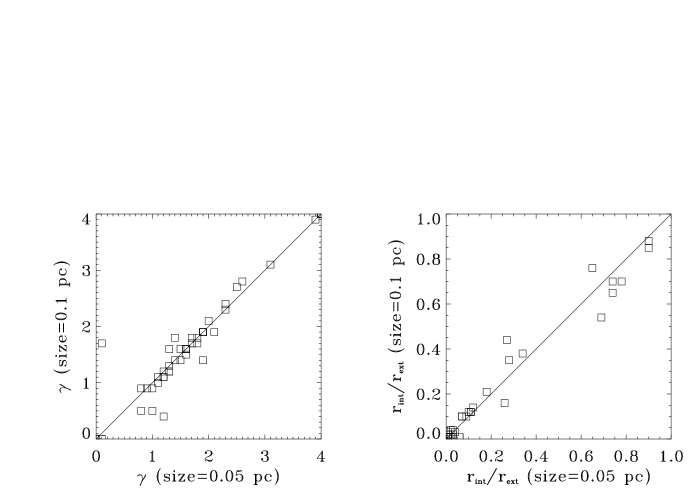
Figure 2: Comparison between the derived model parameters for the two analyzed source diameters (0.1 pc and 0.05 pc). Left panel: index of the power law that describes the density gradient inside the source. Right panel: ratio of internal to external source radii.

Our calculations exhibit a large spread in $EM$ (Fig. 3). HII regions characterized by $EM\geq 10^{7}$ pc cm^-6 are defined as ultra compact. Sources with $EM$ values at the edges of the range do not show any significant difference in their dust emission compared to the other sources of the sample. No relation was observed between infrared colors and $EM$. This physical parameter is also randomly distributed as a function of the Galactic longitude.

The infrared colors of the selected sample follow a typical trend for UCHII regions, while in the radio-millimeter regime not all sources have typical UCHII characteristics, as illustrated by their $EM$ values. Our study in the radio range demonstrates that a sample of UCHIIs selected only on the basis of their infrared colors may be contaminated by other classes of Galactic sources. Planetary nebulae or high-mass evolved stars could have infrared colors similar to those of UCHII, but different ionized gas properties.

5 Estimated detectability with Planck

Planck is equipped with a Low Frequency Instrument (LFI), operating at 30, 44, and 70 GHz and a High Frequency Instrument (HFI) operating at 100, 143, 217, 353, 545, and 857 GHz. To evaluate the fraction of UCHIIs in our sample that is detectable with Planck, we need to compare the modeled flux densities of the sources with the expected sensitivity in each observational band.

We derive the modeled flux densities at each Planck channel from the source SEDs by calculating the dust and gas emission as described in Sects. 4.1 and 4.2 and then summing both contributions. In Fig. 4, four of the derived SEDs are shown as an example; the shaded area represents the spectral range covered by the Planck satellite. The dust contribution was obtained by extrapolating the modified-blackbody fit of the cold dust component (dashed lines in Fig. 4), while the free-free contribution was obtained by modeling the data points as described in Sect. 4.2 and extending the derived synthetic spectra to the submillimeter range (dotted line in Fig. 4).

Figure 3: Comparison of the Emission Measure deduced from the simulation with those calculated from the 7 mm measurements. Arrows refer to those sources optically thick ut to 7 mm.

Following Umana et al., (2006), the expected total sensitivity is assumed to be the sum in quadrature of all the sources of confusion noise, namely (i) the nominal instrumental Planck sensitivity per resolution element, (ii) the extragalactic-foreground confusion noise (Toffolatti et al., 1998), (iii) the CMB anisotropy (Bennett et al., 2003a ), and (iv) the Galactic-foreground confusion noise.

As pointed out by Wood & Churchwell, 1989b , the Galactic distribution of candidate massive-star formation sites is mainly confined to the Galactic plane, and our sample consists indeed of UCHIIs located in the Galactic plane, where we also expect the Galactic emission to be the major source of confusion noise in all Planck channels because of the emission of the dust and gas located in the Galactic disk.

The Galactic noise reported by Umana et al., (2006) was derived for regions of the sky outside of the Galactic plane, therefore we cannot use this value for UCHII regions. For a realistic estimation of the noise related to the Galactic emission, we simulate the sky emission in the range between 30 and 900 GHz with the Planck sky model (PSM) software package (version 1.6.3). PSM is a set of programs and ancillary data developed by the Planck ESA Working Group 2 that can simulate the sky emission at Planck frequencies and angular resolution, and reproduces the thermal free-free, synchrotron, and the dust components, i.e., thermal dust and spinning dust. The free-free component is modeled following Dickinson et al., (2003) and the spatial structure estimated from the dust-extinction corrected $H_{\alpha}$ emission. The synchrotron component is calculated by assuming a perfect power-law with different values of the spectral index in different sky directions, as derived from the 408 MHz (Haslam et al., 1982) and WMAP 23 GHz (Bennett et al., 2003b ) maps. The thermal emission from interstellar dust is assessed following Finkbeiner et al., (1999). The prediction of the rotating grain emission is obtained by multiplying the column densities of the cold neutral medium (Schlegel et al., 1998) with the emissivities calculated using the spinning dust model developed by Draine & Lazarian, (1998).

For the two Planck channels of lower frequency (30 and 44 GHz), the Galactic emission is dominated by the free-free component, whereas for the third channel (70 GHz) the free-free and the thermal dust components are comparable; for the other channels the emission of the thermal dust dominates. The other emission mechanisms provide negligible large-scale contributions.

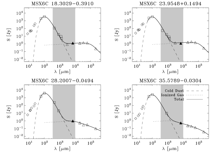
Figure 4: Examples of the source SEDs, different symbols refer to different components. Diamonds: hot dust component; squares: cold dust component; triangles: ionized gas. The dust component is deduced from the template SED, the free-free emission of the ionized gas derived from its model. The spectral range covered by Planck is represented by the shaded area.

To obtain an idea of the trend of the Galactic emission fluctuations as a function of the Galactic longitude, the standard deviation of the Galactic emission for each PSM channel map was calculated in boxes of size $3\times\theta_{\nu}$ ($\theta_{\nu}$ is the Planck beam at the considered frequency), centered on Galactic latitude $0^{\circ}$ and spaced every $5^{\circ}$ in longitude. We selected the size of the region in which the standard deviation of the Galactic emission was to be calculated as a compromise between the necessity both to have a large number of pixels in the region and to remain well inside the plane of the Galaxy. We show the RMS of the Galactic emission for each channel map at different values of Galactic longitude for the two Planck instruments in Fig. 5. The Galactic emission fluctuation strongly depends on the longitude. The first and fourth Galactic quadrants (center) are characterized by higher noise with respect to the second and third quadrants (anticenter), as an obvious consequence of the larger amount of dust in the direction of the center of the Galaxy.

The correctness of the PSM predictions was tested by comparing them to the observed all-sky WMAP temperature map for Stokes I at 41 GHz (Q band). The WMAP data were retrieved from the NASA Legacy Archive for Microwave Background Data Analysis (LAMBDA), while a sky temperature map at the same frequency and angular resolution was constructed with PSM. We found very good agreement between them, allowing us to use our results on the Galactic emission fluctuation with confidence.

In Fig. 6, we show the percentage of objects from our sample that could be detected above the 3$\sigma$ threshold for each channel of the instruments onboard Planck. Unfortunately, all the UCHIIs in our sample are located in the first and fourth quadrants and because of the high Galactic emission fluctuation a very small fraction of them should be detected by Planck.

However, UCHIIs have been detected in any Galactic direction (Wood & Churchwell, 1989b ). Therefore, assuming that our sample is representative of the entire class of UCHIIs, we can also calculate the detectability of those located in the region of the Galactic anticenter. Figure 6 shows how UCHIIs in the direction of the anticenter should be easily seen by Planck.

Unfortunately, the high-mass star-formation rate is expected to strongly decrease far away from the center of the Galaxy. Bronfman et al., (2000) reported that the OB star-formation sites in the anticenter direction reduced to about 10$\%$ those detected in directions close to the center of the Galaxy. The expected increased Planck capability to detect UCHIIs in the anticenter direction has to be compared with the decreasing star formation rate. The true expected number of detectable UCHIIs must be weighted by the radial distribution of star formation in the Galaxy.

The UCHII sample analyzed in this paper represents only a subsample of the 228 UCHII regions reported by Giveon et al., 2005a , which are distributed in a region of the Galactic disk that cover about $52^{\circ}$ of Galactic longitude. Taking into account the estimation of Bronfman et al., (2000), the expected UCHIIs that Planck could detect for a similar range of Galactic longitudes in the anticenter direction could be tens. Note that the Planck channels that have the higher capability of detecting UCHIIs are the channels at the lower wavelengths (Fig. 6), where the dust emission contribution is dominant. However, the sample selected by Giveon et al., 2005a has a bias towards sources above the threshold detectability at the radio wavelengths. Therefore, it is reasonable to expect that the estimation reported here is only a lower limit to the true number of UCHII regions detectable by the Planck satellite, as there may be many sources with very low radio emission levels, for actual sensitivities, but with detectable IR dust emission. We emphasize that this conclusion is supported by many detections of UCHIIs in the region of the Galactic anticenter obtained with the balloon experiment Archeops at mm and sub-mm wavelengths (Desert et al., 2008).

Figure 5: Expected Galactic emission fluctuation for $|b|\leq 0.5^{\circ}$ at different values of Galactic longitude for the two Planck instruments.

In many cases UCHIIs have been observed on the borders of larger and fainter HII regions. In higher wavelength channels, the Planck beam may be large enough to detect emission from these associated normal HII regions. Considering their contribution, the Planck capability to detect UCHIIs here reported could be an underestimate.

We conclude that we expect the Planck mission to provide an important contribution to studies of UCHIIs, as it will provide the scientific community with measurements in a still largely-unexplored spectral region.

6 Summary

We have presented 7 mm (43 GHz) observations of a sample of radio-bright ultra-compact HII regions carried out with the INAF-IRA Noto Radiotelescope. The results of this survey provide a sizeable database of new millimeter measurements that allow us to characterize the high-frequency free-free contribution from the ionized-gas components of the selected targets. The free-free spectrum of each source were derived by modeling all the available radio and millimeter observations and the new 7 mm data.

We used our 7 mm measurements along with infrared and sub-millimeter data to compile SEDs from the radio to the far-IR and to estimate the expected flux densities in the spectral region between the cm and the sub-mm ranges.

Figure 6: Expected Planck capability of detecting the sample of UCHII analyzed here. Dashed line: true source Galactic position. Dot dashed line: results for the same population but located in the anticenter region.

The study of properties of Galactic UCHIIs is one of the secondary science objectives of the Planck core program (The Planck Collaboration, 2005) therefore, it appears to be important to test the capability of Planck to detect UCHII regions. We, thus, estimated the fluctuation of the Galactic emission as a function of the Galactic longitude by using the Planck Sky Model software package. In this paper, we note that we report for the first time a quantitative estimation of the emission fluctuation of the Galactic disk as seen by Planck. As expected, the Galactic emission fluctuation is higher near the center of the Galaxy. When comparing the modeled radio/sub-mm flux densities to the expected total sensitivity of the Planck satellite, we evaluate that few sources are likely to be detected by Planck in the direction of the Galactic center, where the sources of our sample are located. If we assume that the sample analyzed in the present paper is representative of the whole Galactic UCHII population, we infer a higher rate of detectability by Planck in the direction of the Galactic anticenter, where the Galactic emission fluctuation is significantly lower.

Therefore, even though designed for cosmological studies, Planck should also contribute to the UCHII science. The rich source database provided by Planck will allow follow-up observations aimed at the investigating morphological details with future instruments working in the same spectral region, such as ALMA.

The source parameter emission measures were derived both directly from the 7 mm measurements and, independently, from a model of the ionized-gas continuum emission. The derived $EM$ values for each sources are clearly correlated, supporting the goodness of the model fit. The analysis of this parameter leads us to conclude that our sample could be contaminated by other types of Galactic sources, although all of the selected targets can be classified as UCHII regions because of their infrared colors.